The design of IIR filters
4.1 CHAPTER PREVIEW
We are now in a position to consider the various approaches to the design of digital filters. The two types of filter, FIR and IIR, have very different design methods and so will be considered separately. In this chapter we will focus on the techniques used to design IIR or recursive filters. We begin with a very brief résumé of filter essentials.

Figure 4.18
4.2 FILTER BASICS
Before we move on to the design of digital filters, it is probably worth having a very brief recap on filters.
An ideal filter will have a constant gain of at least unity in the passband and a constant gain of zero in the stopband. Also, the gain should increase from the zero of the stopband to the higher gain of the passband at a single frequency, i.e. it should have a ‘brick wall’ profile. The magnitude responses of ideal lowpass, highpass, bandpass and bandstop filters are as shown in Fig. 4.1(a), (b), (c) and (d).
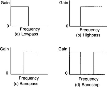
Figure 4.1
It is impossible to design a practical filter, either analogue or digital, that will have these profiles. Figure 4.2, for example, shows the magnitude response for a practical lowpass filter. The passband and stopband are not perfectly flat, the ‘shoulder’ between these two regions is very rounded and the transition between them, the ‘roll-off’ region, takes place over a wide frequency range. The closer we require our filter to agree with the ideal characteristics, the more complicated is the filter transfer function.

Figure 4.2
As the gain of a real filter does not drop vertically between the passband and stopband, we need some way of defining the ‘cut-off’ frequencies of filters, i.e. the effective end of the passband. The point chosen is the ‘−3 dB’ point. This is the frequency at which the gain has fallen by 3 dB, or to 1/√2 of its maximum value (gain in dB = 20 log10 [gain]).
If you are rusty on the basic principles of analogue filters, this would be a good time to do some background reading. Some keywords to look for are: lowpass, highpass, bandstop, bandpass, cut-off frequency, roll-off, first, second (etc.) order, passive and active filters, Bode plots and dB. Howatson (1996) is just one of an abundance of circuit theory and analysis texts which will be relevant.
Much work has been carried out into the design of analogue filters and, as a result, standard design equations for analogue filters with very high specifications are available. However, as has been stressed earlier in this book, the characteristics of all analogue systems alter due to temperature changes and ageing. It is also impossible for two analogue systems to perform identically. Digital filters do not have these defects. They are also much more versatile than analogue filters in that they are programmable.
We will now look at various methods of designing digital filters.
4.3 FIR AND IIR FILTERS
You will remember from earlier chapters that digital filters can be divided broadly into two types – finite impulse response (FIR) and infinite impulse response (IIR) filters. If a single pulse is used as the input for an FIR filter the output pulses last for a finite time, while the output from an IIR filter will, theoretically, continue for ever. Generally, FIR filters are non-recursive, i.e. do not use feedback, while IIR do. It should be pointed out at this stage that it is possible to design some FIR filters which are recursive. However, for convenience, the term FIR filter will be taken to mean a non-recursive filter in this book.
The general expression for the transfer function, T(z), of an FIR filter is:
while that for the IIR filter is:
Although they have the disadvantage of requiring more coefficients to achieve a similar filter performance, FIR filters do have the advantage that they will never be unstable, unlike IIR filters. FIR filters also have the potential to feature a linear phase response – but more on this later. The main point is that the two types of filter are very different in their performance and also in their design. In this chapter we will deal with the design of IIR filters only; FIR filters are considered in the next chapter.
There are several approaches that can be taken to the design of IIR filters. One common method is to take a standard analogue filter, e.g. Butterworth, Chebyshev, Bessell, etc., and convert this into its discrete equivalent. An alternative procedure is to start with the z-plane p–z diagram and attempt to place poles and zeros so as to produce the desired frequency response. This is often called the ‘direct’ design method. We will now look at these two approaches in detail.
4.4 THE DIRECT DESIGN OF IIR FILTERS
With this method, poles and zeros are placed on the z-plane in an attempt to achieve the required frequency response. When designing digital filters in this way there is sometimes an element of ‘trial and error’ involved. Often this is small and just serves to ‘tweak’ the calculated pole–zero positions, so as to improve the response, but at other times it is significant – this is usually when it proves very difficult to calculate the optimum pole–zero positions accurately. The reliance on trial and error has obviously been made much more viable with the increased availability of CAD packages such as MATLAB. These packages allow us to simulate and then modify our designs very quickly.
Once a suitable p–z diagram has been established, the system transfer function can be derived. One of the many pleasures of using digital filters is that it is very easy to convert the transfer function into the actual filter, i.e. to convert it into the corresponding DSP software. This is far from true with analogue filters. Here, once we arrive at a suitable p–z diagram, the corresponding transfer function then needs to be converted into suitable hardware – i.e. electrical components. This is a much more difficult task!
This ‘direct’ method of IIR filter design is best described by means of examples, and so two follow.
Example 4.1
A lowpass digital filter is required that has a d.c. gain of 1 and a cut-off frequency which is 0.25 of the sampling frequency. The filter is to have a transfer function of the form T(z) = k(z + a)/(z + b).
Solution: Our first task is to locate the single zero and pole. To complete the design we then need to calculate a suitable k-value.
As we require a lowpass filter then, after the initial passband, the gain must fall as the frequency increases, i.e. as we move around the z-plane unit circle in an anticlockwise direction, starting at z = 1 (d.c).
it would therefore be sensible to arrange for the zero distance to be zero at the Nyquist frequency. In other words, we will need to place the filter zero at z = −1.
Common sense suggests that, in order to achieve the required response, the single pole probably needs to be placed somewhere on the positive real axis, i.e. this will ensure a large gain for low frequencies and a lower gain for high frequencies. Figure 4.3 shows the zero at z = −1 and the pole at z = d. Point A corresponds to 0 Hz and point B to the cut-off frequency, which is half the Nyquist frequency (a quarter of the sampling frequency).

Figure 4.3
the gains at 0 Hz and 0.5fN are given by:
But B is the −3 dB point, therefore

Therefore the pole must be placed at the origin.
Applying
at point A:

Substituting the a-, b- and k-values into the transfer function gives us:
Figure 4.4 shows that the −3 dB point does occur at 0.5fN and that the d.c. gain is 1 (0 dB), and so our design has satisfied the filter specification.

Figure 4.4
Example 4.2
A digital notch filter is required which has a notch frequency of 20 Hz, a bandwidth of no more than 4 Hz and an attenuation at the notch frequency of at least 40 dB. The gain in the passband is to be 1. The sampling frequency is 160 Hz.
Solution: A notch filter is a very narrow bandwidth bandstop filter – it has a gain which drops and then rises very steeply with increasing frequency and so the magnitude response has the shape of a notch.
it follows that we must make the ‘zero distance’ very small at the notch frequency. As the specification stipulates that the attenuation needs to be at least 40 dB then the easiest thing to do is to place a zero on the unit circle at the position corresponding to the notch frequency of 20 Hz. This, theoretically, should cause the gain to fall to zero. This z-plane zero will, of course, be one of two complex conjugate zeros.
As the sampling frequency is 160 Hz then the Nyquist frequency is 80 Hz and so the notch frequency of 20 Hz corresponds to an angle of 45° on the z-plane diagram. Figure 4.5 shows the zero, Z, along with its complex conjugate zero, placed on the unit circle at the position corresponding to this frequency.

Figure 4.5
We now need to place the complex conjugate poles so that we obtain the correct bandwidth of no more than 4 Hz. In other words, the gain must fall to −3 dB, or to approximately 1/√2 of its passband gain, at 18 Hz and 22 Hz.
From the symmetry of the frequency response, it seems sensible to place the poles on the same radii as the zeros. The two poles will have to be sufficiently close to the corresponding zeros to ensure that the gain is approximately unity for all of the frequency range, apart from the ‘notch’. As they are so close then k = 1 is required to give a passband gain of 1. Their locations must also be such that the bandwidth is 4 Hz. We might find that this specification is impossible to achieve.
In Figure 4.5 the two poles are shown as being a distance d away from the two zeros. Also shown are the two −3 dB points, B and A, at 18 Hz and 22 Hz respectively (not to scale).
The angle ACB corresponds to 4 Hz and so, as fN = 80 Hz,
Using s = rθ, where s is the arc of a circle, r the radius, and θ the angle subtended by the arc, then, as r = 1, the arc length from A to B must also be 0.16, and so ZA = ZB = 0.08.
As A is very close to Z, the pole, the zero and A (or B) form an approximate right-angled triangle, with ∠AZP ≈ 90°. Therefore the pole distance from A or B must be very close to ![]() .
.
and k = 1,
Therefore, the poles must be 0.92 from the origin.
It follows that we must place the zeros at cos 45° ± j sin 45°, i.e. at 0.707 ± j0.707, and the poles at 0.92 cos 45° ± j 0.92 sin 45° or 0.651 ± j 0.651.
N.B. The effect of the other pole and zero has not been taken into account in the calculation. This is because they are so close together that they tend to cancel each other out and so should not affect the gain significantly.
The design is now complete; all that remains is to check the response – the MATLAB plot is shown in Fig. 4.6. It can be seen that the magnitude response satisfies the specification, with the notch frequency occurring at 0.25fN (20 Hz), the notch attenuation being at least 40 dB and the bandwidth approximately 0.05fN (4 Hz).

Figure 4.6
If we had found that the response was not satisfactory then the pole positions could easily be ‘tweaked’, with the help of MATLAB, in order to improve the performance.
N.B. We probably overdid the calculation in these examples and, practically, could have relied more on MATLAB to decide on the location of the poles and zeros. For example, once we had calculated the zero positions in the ‘notch’ problem, we could have found suitable positions for the poles by trial and error, which would have saved a lot of work. However, it is important that you understand the underlying principles in the design process, and so the extra calculations were worthwhile – no doubt you feel much better for having done it?
4.5 SELF-ASSESSMENT TEST
A discrete bandpass filter is required that has a centre frequency of 100 Hz, a bandwidth of 20 Hz and a peak gain of 1. The filter is to have a transfer function of the form T(z) = k/(z2 + a2) and the sampling frequency is 400 Hz.
4.6 RECAP
• The direct method for the design of IIR filters relies on poles and zeros being placed at suitable points in the z-plane so as to achieve an adequate frequency response.
• Some calculation is usually needed for the initial location of the poles and zeros but the final fine-tuning can often be done with the help of suitable software, i.e. by using ‘trial and error’.
4.7 THE DESIGN OF IIR FILTERS VIA ANALOGUE FILTERS
The direct design method can give reasonable results for fairly simple filters. However, it is far from ideal when something rather more sophisticated is needed, and so an alternative approach is required.
A huge amount of research has been carried out in the past into the design of analogue filters and, as a result, ‘classic’ filters such as Butterworth, Chebyshev, ‘elliptic’ etc. have been developed, each one having its own particular good and less good features. A modern-day designer of analogue filters therefore has an excellent library of designs at his or her disposal. It would be a dreadful waste of effort not to try to make use of this expertise when designing digital filters. Very sensibly, various s-domain to z-domain transforms have been developed which allow us to convert analogue filters into their digital ‘equivalents’ fairly easily. It must always be remembered that all transforms are approximations and that no digital filter can be identical to its analogue prototype, i.e. have exactly the same magnitude, phase and time responses. The various s-to-z transformation methods have advantages and disadvantages. Remember also that a digital filter should not be expected to operate above the Nyquist frequency – this is clearly not a consideration when building analogue filters.
There are many standard methods of converting an analogue filter to its digital equivalent – a process called ‘discretization’. We will look at three of the most common – the bilinear transform, the impulse-invariant method and the pole–zero matching technique.
4.8 THE BILINEAR TRANSFORM
I mentioned earlier that there are classic analogue filters which we can use as templates when we need to design a digital filter. However, some of these have fairly complicated s-domain transfer functions and so, to save having to deal with unnecessarily complicated algebra at this stage, a very simple filter will be used to demonstrate the various conversion methods. The prototype filter that will be used is a first-order, lowpass filter having the transfer function:
(The filter is classed as a first-order filter as the highest power of s is 1. Generally, the higher the order the better the filter performance.)
This transfer function defines a lowpass filter with a cut-off angular frequency of ωc rad/s. For example, if we choose ωc = 10 rad/s, then:
or
Figure 4.7 confirms the predicted frequency response of the filter, i.e. it is a lowpass filter with a cut-off frequency of 10 rad/s (or approximately 1.6 Hz).
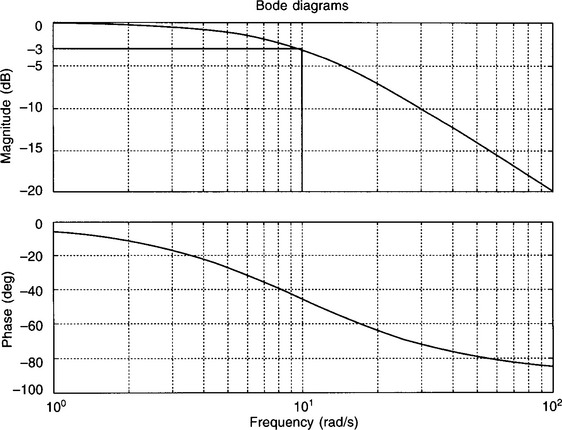
Figure 4.7
To apply the bilinear transform we have to replace s with:
where T is the sampling period. (See Virk (1991), Oppenheim and Schafer (1975) or Ludeman (1987) for an explanation of the origin of this transform.)
We will now convert the analogue lowpass filter to its discrete equivalent using a sampling frequency of 16 Hz (T = 0.065 s).

The frequency response for this filter is shown in Fig. 4.8.
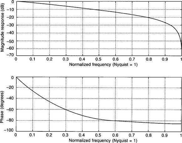
Figure 4.8
Taking into account the linear frequency scale, the phase response has roughly the same shape as that of the analogue filter, while the magnitude response appears to be in very good agreement – it is certainly a lowpass filter! However, a more detailed examination reveals that the cut-off frequency is approximately 0. 19fN, or 1.5 Hz, rather than the 1.6 Hz (0.2fN) of the analogue filter, which is an error of approximately 6%. This is a recognized problem associated with the bilinear transform, i.e. breakpoint frequencies might be changed significantly during the transformation.
However, all is not lost. If the approximation is too poor to be acceptable, then we need to ‘pre-warp’ the frequencies before we apply the bilinear transformation. This entails modifying the s-domain transfer function in a particular way, such that the gain at a ‘frequency of interest’ (usually an important breakpoint) is the same for the discrete filter as the continuous filter. (N.B. Frequency pre-warping does not change the d.c. gain.)
If the frequency at which we want to equate the gains is ωc, then we first need to calculate a ‘pre-warped’ version, ![]() , where:
, where:
In this example we have just one frequency which is of obvious interest – the single breakpoint of 10 rad/s.
We now need to redesign the digital filter starting with the ‘pre-warped’ s-domain transfer function. There are several ways of doing this, but the easiest is to first change the format of the transfer function such that every s is replaced with s/ωc.
So, dividing numerator and denominator by 10, our simple transfer function now becomes:
The final step is to replace all s/ωc terms with ![]() , i.e. with s/10.34 in our example.
, i.e. with s/10.34 in our example.

We now apply the bilinear transformation to this pre-warped version of the transfer function. This gives:
Figure 4.9 shows the magnitude response before and after pre-warping. The normalized frequency scale has been expanded so as to make the difference between the responses more obvious. The new cut-off frequency now corresponds much more closely to the 0.2fN or 1.6 Hz required.
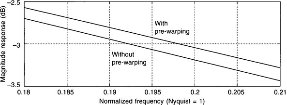
Figure 4.9
Example 4.3
A continuous filter has a transfer function of
It is to be converted to its digital equivalent using the bilinear transform. It is important that the gain is preserved at the upper breakpoint frequency of 2 rad/s. The sampling frequency used is 2 Hz.
Solution: We first need to check whether pre-warping is necessary to maintain the breakpoints. Using
As the difference between ![]() and ωc is significant (about 10%), then pre-warping is necessary.
and ωc is significant (about 10%), then pre-warping is necessary.
Changing the format of the transfer function by replacing all s-values with s/ωc, i.e. s/2, gives:
(Here we have divided both bracketed terms by 2, in other words we have divided the denominator by 4. We therefore also need to divide the numerator by 4 – hence the ‘0.5’.)
Replacing all s/2 terms with s/2.19:
Applying the bilinear transform, i.e. replacing s with 4(z − 1)/(z + 1), results in the z-domain transfer function of:
4.9 SELF-ASSESSMENT TEST
Convert the filter with the transfer function of T(s) = 16/(s + 4)2 into its discrete equivalent, using the bilinear transformation. The discrete filter is to be used with a sampling frequency of 5 Hz.
4.10 THE IMPULSE-INVARIANT METHOD
The approach here is to produce a discrete filter that has a unit sample response which is ‘the same’ as the unit impulse response of the continuous prototype, as shown in Fig. 4.10. Clearly, the output from the digital data processor will be a sampled response, however, if properly designed, the envelope of the signal should be the same as the unit impulse response of the analogue filter.

Figure 4.10
Using our prototype lowpass filter as an example, we start with:
If we use a unit impulse as the input then the Laplace transform of the output, i.e. the ‘unit impulse response’, is also 10/(s + 10). This is because the Laplace transform of a unit impulse is ‘1’ and so Y(s) = T(s) × 1.
If we now find the inverse Laplace transform, y(t), then this tells us the shape of the unit impulse response in the time domain.
From the tables, the inverse Laplace transform of 1/(s + a) is e–at, which is an exponentially decaying d.c. signal.
The final step is to find the z-transform, Y(z), of this time variation. Again, from the Laplace/z-transform tables, e−at has a z-transform of z/(z − e−aT). As the sampling frequency is 16 Hz,
This function must also be the z-domain transfer function, T(z), of our equivalent discrete filter. This is because the z-transform of a unit sample sequence is also 1, and so Y(z) = T(z) ×1. In other words, if we inputted a unit sample sequence into a discrete filter having a transfer function of 10z/(z − 0.535), the z-transform of the output would also be 10z/(z − 0.535). This is exactly what we require of the discrete filter.
To make sure that no mistakes have been made during the transformation, it’s worth checking the unit impulse response and unit sample response of the continuous and discrete filters, respectively. Figure 4.11 shows the impressively close agreement between them – the continuous response plot passing through the circles of the discrete response ‘stems’, so confirming that the transformation has been carried out correctly.
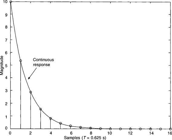
Figure 4.11
Figure 4.12 shows its frequency response – this doesn’t look quite so good! Comparing with Fig. 4.7, the phase response is clearly very different. The phase response is important but not as much as the magnitude response – we will discuss phase response more in the next chapter and will concern ourselves solely with the magnitude response here. Although the −3 dB point on the magnitude response is close to 0.2 fN, i.e. the normalized frequency which corresponds to 1.6 Hz, the gain values are much bigger than we might have expected. However, we could have predicted this gain ‘mismatch’ from an examination of the discrete filter’s p–z diagram, Fig. 4.13.
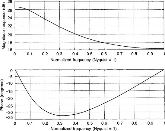
Figure 4.12
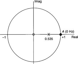
Figure 4.13
gives a d.c. gain of 10/0.465, or approximately 21.5, rather than the ‘1’ which we require for the filter. Luckily, this is not a major problem as we can just scale our transfer function by 1/21.5. The transfer function now becomes:
The new magnitude response is shown in Fig. 4.14. This now gives good agreement with the required response, especially well away from the Nyquist frequency of approximately 50 rad/s.
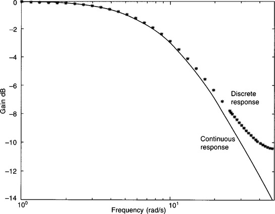
Figure 4.14

Example 4.4
An analogue filter has the transfer function, given by:
Convert this to its discrete equivalent by using the impulse-invariant transform. The sampling frequency is 20 Hz.
Solution: The first thing to do is to try to identify a function of this ‘shape’ in the Laplace transform tables. Unfortunately this one doesn’t appear. What we must therefore do is break it down into functions that do appear, by using the method of partial fractions, i.e.:
By using the ‘cover-up rule’, or any other method, you should find that A = −6, and B = 12,
Using the Laplace/z-transform tables to convert to the z-plane gives us

We now need to make the gains of the two the same at 0 Hz. We could do this by first plotting the two p–z diagrams for the filters and then finding the gains of the two filters at 0 Hz from the pole and zero distances. However, there is no need to do this as we can derive the d.c. gains of the two filters directly from their transfer functions.
Remembering that s = 0 and z = 1 correspond to a frequency of 0 Hz in the s-domain and z-domain respectively, we require to find the value of k, such that:

4.11 SELF-ASSESSMENT TEST
Two analogue filters have the following transfer functions. Convert them to their digital equivalents, using the impulse-invariant transformation.
Assume a sampling frequency of 10 Hz.
4.12 POLE–ZERO MAPPING
The approach adopted here is to use the relationship z = esT to convert the s-plane poles and zeros of the continuous filter to equivalent poles and zeros in the z-plane. Once the z-plane poles and zeros are known, the general form of the z-domain transfer function can be derived. All that then remains to be done is to ensure that the two filters have the same gain, at least at some important frequency – often 0 Hz.
Once again we will use our prototype lowpass filter, with the transfer function of T(s) = 10/(s + 10), to illustrate this method, along with a sampling frequency of 16 Hz.
This particular filter has just a single pole at s = −10. So, using z = esT:
It follows that our equivalent discrete filter has a z-domain transfer function with the general form of T(z) = k/(z − 0.535).
We now need to find the value of k which will make the gains of the two filters the same at a particular frequency. As it is a lowpass filter, it makes sense to use 0 Hz.
Therefore, the transfer function of our equivalent discrete filter is given by:
N.B. Although this method is a very simple one, it generally gives poorer results than the two others, i.e. the bilinear transform and the impulse-invariant method. One disadvantage is that if the prototype continuous filter has no zeros then the discrete ‘equivalent’ will have no zeros. This is not true with the two other conversion methods. This might not seem to be a major problem but zeros are useful in that they help to shape the frequency response of the discrete filter. For example, they can increase the rate at which roll-off occurs. To get around this problem, zeros are often added to ‘all-pole’ filters so as to balance the number of poles – these zeros are usually placed at z = −1. This makes sense because all-pole analogue filters will be lowpass or bandpass filters (draw some pole diagrams to convince yourself of this) and so the equivalent digital filter must have a low gain at the Nyquist frequency.
Our filter design should therefore be improved if we add a single zero at z = −1. The transfer function now becomes:
For the d.c. gains of the continuous and discrete filters to be the same, we require that k = 0.233.
Occasionally the gains need to be equalized at a frequency other than 0 Hz. This is a bit more difficult and so an example is in order.
Let’s say that we have an analogue filter with a transfer function of s/(s + 1). If we convert this to its digital equivalent using the pole–zero mapping method and assuming a sampling frequency of 5 Hz, say, then you should find that the z-domain transfer function is given, approximately, by T(z) = k(z − 1)/(z − 0.82).
Anyway – back to the problem. It doesn’t make very much sense to try to equalize gains at 0 Hz, as they are already the same, i.e. zero. Here we need to equalize the gains at a frequency in the passband. We could do this using MATLAB, or from the p–z diagram, or directly from the transfer function – the latter approach will be taken here.
Theoretically, the gain of the analogue filter never quite reaches 1. However, if we choose an angular frequency which is much greater than the cut-off frequency, then this should be well into the passband region. As the cut-off frequency is 1 rad/s then a frequency of 10 rad/s should be suitable. Substituting this value into the s-domain transfer function, i.e. replacing s with j10, gives a gain of 0.995, which is close enough to 1. We also need to check that this frequency is not above the Nyquist frequency. We are sampling at 5 Hz and so the Nyquist frequency is 2.5 Hz, or approximately 16 rad/s. It follows that our choice of 10 rad/s should be fine.
We therefore need to equalize the gains of the two filters when s = j10. Using z =esT, the corresponding z value is ej2. Using Euler’s identity, z = cos 2 + j sin 2 = −0.416 + j0.91.

N.B. As this is a highpass filter, it would have made more sense to have just equalized the gains at the Nyquist frequency, i.e. at s = j16 and z = −1. This would have also been easier to do. However, if it were a bandpass filter, then we would have no choice but to equalize the gains at a frequency in the passband.
4.13 SELF-ASSESSMENT TEST
Convert the filters with the following transfer functions to their discrete equivalents, using the pole–zero mapping method. The gains of the digital filters are to be made the same as their analogue prototypes at 0 Hz. The digital filters are to be used with a sampling frequency of 10 Hz.
4.14 MATLAB AND s-TO-z TRANSFORMATIONS
Very conveniently, MATLAB has special functions that will perform the main s-to-z transformations for us. This ‘c2dm’ function will automatically generate the appropriate z-domain transfer function coefficients.
For example, if we wish to check our s-to-z conversion of the simple lowpass filter (T(s) = 10/(s + 10)) using the pole–zero mapping method, say, then the MATLAB program is:
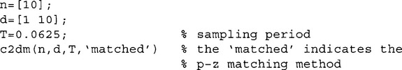
The bilinear transform, both with and without pre-warping, can also be performed. The bilinear transform can also be achieved using the ‘bilinear’ function, while the ‘impinvar’ function can be used to accomplish the impulse-invariant transformation. Consult the MATLAB user manual for further details.
4.15 CLASSIC ANALOGUE FILTERS
So far we have looked at how to convert some fairly simple analogue filters to their discrete equivalents. As mentioned earlier, there are many standard analogue filter types available to us as prototype filters. In other words, if we need to design a digital filter with a certain maximum ripple in the stopband and passband, a particular rate of roll-off etc. we do not have to start from scratch. All we need to do is select one of the classic filters, e.g. Butterworth, Chebyshev, etc., which best satisfies the specification and then use a suitable s-to-z transformation method to convert it to the equivalent digital filter.
It is not the aim of this text to cover the very important, but lengthy topic of analogue filters – here we are only concerned with how to convert a suitable analogue filter to its digital equivalent. If you have not met the standard filter types then you are advised to do some background reading. There are many books available on this topic but you will probably find Ingle and Proakis (1997), Steiglitz (1995) and also Denbigh (1998) particularly helpful as these texts also deal with the conversion of standard analogue filters to their digital equivalent. (Keywords: Butterworth, Chebyshev, elliptic, Bessell, pass/stopband ripple.)
I would not want to leave this particular approach to digital filter design without converting one of the classic prototypes to its discrete equivalent. The following worked example is based on a Butterworth filter. The main advantage of this particular family of filters is that they have very flat stop- and passbands. The major disadvantage is that the initial roll-off rate is fairly slow. In other words, the ‘shoulder’ between the pass and stop regions is rather rounded compared to some other filter types such as the members of the Chebyshev family. Chebyshev filters, in turn, have the drawback of a relatively large ripple in the passband or the stopband.
Example 4.5
A second-order, lowpass Butterworth filter has the following transfer function:

where ωc is the cut-off angular frequency.
Using this as a prototype, design a lowpass digital filter, having a cut-off frequency of 70 rad/s. The bilinear transform is to be used for the conversion and the filter is to be used with a sampling frequency of 100 Hz.
Solution: We first need to check whether pre-warping is necessary.
This is significantly different from ωc and so pre-warping is worthwhile.
Replacing ωc with ![]() in the filter transfer function:
in the filter transfer function:
Using the bilinear transformation, i.e. s = 2(z − 1)/T(z + 1):

Figure 4.15 compares the digital and analogue gain responses. As expected, the filter responses agree closely at lower frequencies but begin to diverge as the Nyquist frequency of 50 Hz (314 rad/s) is approached.

Figure 4.15
4.16 FREQUENCY TRANSFORMATION IN THE s-DOMAIN
You have probably noticed that all but one of the discrete filters we have designed, so far, have been lowpass filters. The reason for concentrating on this particular class of filter is that the transfer function for a lowpass filter can be used as a template for the design of other types, i.e. highpass, bandpass and bandstop. In other words, if we know the expression for the transfer function of a second-order, lowpass, Chebyshev filter, for example, then we can use it to derive the transfer function for a second-order, bandpass, Chebyshev filter. This is because there are standard transformations (yet again!) which can be used to convert the transfer function of a lowpass filter into the transfer function for any other filter type within that family of filters.
For example, if we wish to convert a lowpass filter with a cut-off angular frequency of ωc to a highpass filter with a cut-off angular frequency of Ωc, then we just need to replace s, in the s-domain transfer function for the lowpass filter with:
To demonstrate this we will use our old friend, the simple lowpass filter with the transfer function of T(s) = 10/(s + 10). This lowpass filter has a cut-off frequency of 10 rad/s. Let’s imagine that we want to design a simple first-order, highpass filter with a cut-off frequency of 6 rad/s.
We therefore need to replace s with 10 × 6/s, to produce our transfer function, TH(s), for the highpass filter.
The magnitude response, Fig. 4.16, is clearly that of a highpass filter with a cutoff angular frequency of 6 rad/s.
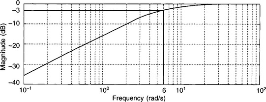
Figure 4.16
We can save ourselves much hard work by using the MATLAB functions lp2lp, lp2hp, lp2bp and lp2bs to convert the transfer function of a continuous lowpass filter into that for another lowpass or highpass, bandpass and bandstop filter, respectively.
For example, the MATLAB program
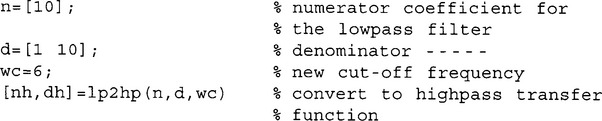
will generate the transfer function coefficients for our simple, first-order, highpass filter.
4.17 FREQUENCY TRANSFORMATION IN THE z-DOMAIN
In the above example, the conversion from lowpass to highpass filter was carried out in the s-domain. To produce the digital version of this we would then need to convert this highpass analogue filter to its digital equivalent using one of the various methods available to us, possibly with the help of MATLAB. However, if we know the z-domain transfer function for the discrete lowpass filter then this change from lowpass to highpass (or to any other type) can also be done directly in the z-domain.
To make this conversion from a lowpass to a highpass digital filter we have to replace z with:
where
and ωc and Ωc are the cut-off angular frequencies for the low and highpass filters respectively.
As an example, we will transform the discrete equivalent of our lowpass filter with the s-domain transfer function T(s) = 10/(s + 10). We will use the z-domain transfer function obtained earlier using the impulse-invariant technique (Section 4.10), i.e T(z) = 0.465z/(z − 0.535). Again, a highpass filter with a cut-off frequency of 6 rad/s will be aimed for. The sampling frequency is 16 Hz (T = 0.0625 s).

Replacing z with − (1 − 1.13z)/(z − 1.13) in T(z) = 0.465z/(z − 0.535):

Figure 4.17 shows the frequency response of this filter. It is a highpass filter with a cut-off frequency which is very close to 0.12fN, i.e. 0.96 Hz or 6 rad/s.
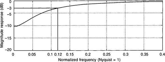
Figure 4.17
| N.B.1 | Although we have looked at a fairly simple example, any type of lowpass filter can be changed to another lowpass filter of different cut-off frequency or to equivalent highpass, bandpass or bandstop filters. The formulae for all conversions, both in the s-domain and the z-domain, are shown in Appendix B. |
| N.B.2 | We have worked manually through the various steps of this particular approach to filter design, just relying on MATLAB to perform some stages of the design and also to check the performance of our filters. However, we can also use MATLAB to carry out the complete design for us. Once a decision has been made as to which family of filters is required, e.g. Butterworth, Chebyshev etc., the filter specification can then be entered and MATLAB will respond by generating the discrete filter transfer function coefficients directly. |
| For example, ‘[nz, dz] = butter(3, 0.4, ‘high’)’ will generate the transfer function coefficients for a Butterworth, third-order, highpass filter, with a cut-off frequency equal to 0.4 × fN, where fN is the Nyquist frequency. If we add ‘freqz(nz, dz)’, to the program, the frequency response (Fig. 4.18) will also be plotted. This facility is obviously invaluable when it comes to the practical design of digital filters. Refer to the MATLAB user manual for further details. |
4.18 SELF-ASSESSMENT TEST
A lowpass digital filter has a transfer function of 0.15 (z + 1)/(z − 0.7). Given that this filter has a cut-off frequency of 55 Hz when sampled at a frequency of 1 kHz, use the table of Appendix B to convert it to a highpass filter with a cut-off frequency of 100 Hz. Assume a sampling frequency of 1 kHz.
4.19 RECAP
• A common way of designing IIR filters is to base the design on a suitable analogue filter. The prototype filter is often one of the tried and trusted classic filters such as Butterworth, Chebyshev etc. Each one of these filters has its own particular good and bad points and the initial choice of filter is a very important stage of the design process.
• Transformations such as the bilinear (often with pre-warping), pole–zero mapping and the impulse-invariant can then be used to convert the s-domain transfer function into its z-domain equivalent.
• Designs are usually based on a prototype of a lowpass filter. This is because the transfer function for all other types, i.e. highpass, bandpass, bandstop and lowpass filters with different cut-off frequencies can be derived from the transfer function of a lowpass filter by using yet more transformations.
• CAD packages are available which, once given the desired filter specification, will generate the transfer function of the digital filter for us directly.
4.20 PRACTICAL REALIZATION OF IIR FILTERS
Once the design process has been completed and simulation carried out to check the design, the final step is to program the DSP system, i.e. to write the controlling software. The essential data that must be entered into the program are the transfer function coefficients and the sampling frequency. In Chapter 2, the transfer function was derived for a general recursive filter. This has the form of:
The transfer function coefficients must usually be entered into the DSP software in this form. For example, if we have a filter with a transfer function of:
then the format needs to be changed to:

Dividing numerator and denominator by z2 in order to change all indices to negative values and the initial value of the denominator to 1:
Therefore, comparing with the general transfer function (equation (4.1)), a0 = 0, a1 = 0.4, a2 = −0.12 and b1 = −0.3, b2 = +0.1 (not +0.3 and −0.1).
I should add a word of warning at this point. There can be unexpected problems with the filter performance if the coefficients are entered directly in this format. This is particularly likely when the sampling rate is very large compared to the filter breakpoints. This is because the filter poles and also the zeros tend to cluster together as fs increases. In other words, the roots of the numerator and also the denominator polynomials become very close. To convince yourself of this, convert a filter with a transfer function of (s + 2)/(s + 1)(s + 3) into its z-plane equivalent using the bilinear transform and a sampling frequency of 20 Hz, 200 Hz and 2000 Hz. You should find that the poles (and the zero) move closer and closer to z = +1 as the sampling frequency increases. Remember that, practically, there are a limited number of bits available in a processor to store each coefficient and so ‘rounding’ of coefficient values inevitably take place during processing. These approximation errors obviously become extremely significant when the roots of the polynomials are so close. A pole which should be near to the unit circle could even be calculated as being just outside – i.e. disaster! To overcome this ‘clustering’ problem, the filter is often broken down into smaller sections which are then cascaded to produce the complete filter. It can be shown that this structure reduces the problem. For more information on this method of implementation see Steiglitz (1995) and also Ingle and Proakis (1991, 1997). (Keywords: biquadratic sections.)
Hopefully, you are now in a position to do some practical designing and testing of IIR filters. Unfortunately, in a book of this length, it is not feasible to deal with the practical details of programming specific DSP systems – for this you will need to consult the appropriate user manual. Several very useful books have also been written which concentrate on practical applications of particular processors, e.g. El-Sharkawy (1996), Ingle and Proakis (1991) and Chassaing and Horning (1990).
4.21 CHAPTER SUMMARY
In this chapter we began with a very brief review of analogue filters, emphasizing that the frequency responses of real filters are usually a long way from that of ideal filters. We then looked at two general methods of designing IIR filters. The first was the ‘direct’ method. This entails placing poles and zeros in the z-plane so as to ‘mould’ the frequency response into the required shape. The approximate locations of the poles and zeros can be arrived at by calculation and then fine adjustments made to improve the response. Suitable CAD packages are invaluable when adopting this approach to filter design.
This direct method is fairly rough and ready and not feasible when a filter with a very ‘tight’ specification is required. We would then have to turn to the second approach, i.e. base the design on a suitable analogue filter. The analogue prototype, which will often be one of the ‘classics’, would then have to be converted to its digital equivalent using one of the various s-to-z transformations. Filter designs are usually based on lowpass filters as these can be readily converted to other types, both in the s-domain and the z-domain.
CAD packages are available which will carry out the complete design process.
4.22 PROBLEMS
1. A highpass filter is to be designed, using the ‘direct’ method, i.e. by placing transfer function poles and zeros at suitable points in the z-plane. The filter is to have a transfer function of the form T(z) = k(z − 1)/(z − a), a cut-off frequency which is 0.125 of the sampling frequency (0.25fN), and a gain of 1 at the Nyquist frequency.
2. Continuous filters with transfer functions of:
are to be converted to their digital equivalents. The bilinear transform is to be used, with pre-warping. Both continuous filters have breakpoint frequencies of 5 rad/s and this breakpoint is to be retained by the discrete filters, i.e. this is the frequency which must be pre-warped. Both filters are to be used with a sampling frequency of 8 Hz.
3. Convert the filter with the transfer function of T(s) = s/(s + 4) to its discrete equivalent using pole–zero mapping. The filter is to be used with a sampling frequency of 4 Hz. The transfer function of the discrete filter must be scaled such that it has the same gain as the continuous filter at 2 Hz (fN). (N.B. This is a highpass filter.)
4. The following transfer functions are for two lowpass, continuous filters. Use the impulse-invariant transformation to convert them to the transfer functions of equivalent discrete filters. The discrete filters must have the same d.c. gains as the corresponding analogue filter. The discrete filters are to be used with a sampling frequency of 5 Hz.
5. A lowpass analogue filter has a transfer function of T(s) = 3/(s + 3). This transfer function is to be converted to one for a discrete, highpass filter, with a cut-off frequency of 6 rad/s. The filter is to be used with a sampling frequency of 10 Hz and the conversion is to be done by:
(a) changing from lowpass to highpass in the s-domain and then converting to the discrete, equivalent highpass filter by using the pole–zero mapping technique. (The discrete highpass filter must have the same gain as the continuous filter at the Nyquist frequency.)
(b) converting to an equivalent discrete, lowpass filter using the pole–zero mapping method (the added zero is to be placed at z = −1) and then converting from lowpass to highpass in the z-domain. (The continuous lowpass filter and its discrete equivalent must have the same d.c. gains.)