
The z-plane
3.1 CHAPTER PREVIEW
We start this chapter with a review of the s-plane, a concept with which you are probably familiar. We will then move on to its discrete equivalent – the z-plane. The z-plane has an extremely important role to play in the design and analysis of discrete systems. The significance of z-plane pole–zero diagrams will be discussed, both in terms of signal shapes and system frequency response. The link between the s-plane and z-plane will also be examined.
3.2 POLES, ZEROS AND THE s-PLANE
It is very likely that you have already encountered the ‘s-plane’. If so, you will appreciate how useful this concept is when it comes to the analysis and design of analogue systems. In a similar way, the z-plane is an invaluable tool when it comes to the analysis and design of discrete systems. As it’s much easier to explain the significance and the use of the z-plane via the s-plane, we will begin with a very brief review of the s-plane. If you are completely at ease with the Laplace transform, the s-plane, and the idea of poles and zeros, then you can probably afford to skip the next few pages. However, if you know little about these, or are very rusty, then you will need to do some extra reading, as it is unlikely that the following review will be sufficient for you. You will find comprehensive explanations in most textbooks dealing with circuit analysis and control systems in particular. Just three of many suitable sources are Bolton (1998), Powell (1995), and Dorf and Bishop (1995).
The s-plane is simply an Argand diagram, used to display the values of s. Remember that s represents the complex frequency, i.e. s = σ + jω, and so s values can be naturally shown on an Argand diagram. As is usual for Argand diagrams, the real part of s, i.e. σ, is plotted along the horizontal axis and the imaginary part, jω, along the vertical axis.
As an example, consider a continuous system with a transfer function given by:
This transfer function can be represented on an s-plane diagram by displaying its poles and zeros (Fig. 3.1).

Figure 3.1
System zeros are the s-values that cause the numerator, and so T(s) itself, to become zero, while poles are defined as the values of s which result in T(s) becoming infinite, i.e. its denominator becoming zero. It follows that this particular transfer function has a single zero at s = −4 and two poles at s = −2 and −3. On pole–zero diagrams, poles are traditionally represented by crosses and zeros by circles.
In this simple example all values are real and so appear on the real (σ) axis – but what if the transfer function had been more complicated? For example,
We will begin by finding the zeros for this transfer function and so must first equate the numerator to zero, i.e. s2 + 2s + 5 = 0. As this quadratic expression factorizes to (s + 1 + j2)(s + 1 − j2), then the system must have complex conjugate zeros at s = −1 ± j2.
To find the poles we need to examine the denominator. Clearly, there must be one pole at s = −3 (this is obviously a real pole). Also, as s2 + 2s + 2 factorizes to (s + 1 + j)(s + 1 − j), there must be two complex conjugate poles at s = −1 ± j.
The pole–zero diagram for this system is shown in Fig. 3.2.

Figure 3.2
Pole–zero diagrams of system transfer functions contain a surprising amount of information about the system and are extremely useful when it comes to the design and analysis of signal processors. For example, it can be shown that a system with poles in the right-hand half of the s-plane is an unstable system. We will examine system pole–zero diagrams in much more detail later in the chapter.
3.3 POLE–ZERO DIAGRAMS FOR CONTINUOUS SIGNALS
As signals can also be transformed into the s-domain, i.e. expressed as functions of s, then they too can be represented by pole–zero diagrams. These ‘p–z’ diagrams contain information about the signal shapes and so are very useful.
To illustrate this important link between the signal p–z diagram and the signal shape consider a signal, y(t), having a Laplace transform, Y(s), given by:
We will first find the time variation of the signal by using the traditional ‘inverse Laplace transform’ method. However, before the Laplace transform tables can be consulted the expression needs to be broken down into its partial fractions, i.e.:
(You are strongly advised to derive this expression for yourself.)
By inspection of the Laplace transform tables (Appendix A), you should find that the 1/(s + 2) part corresponds to a signal in the time domain of e−2t.
As the other component can be expressed, very conveniently, as 2(s + l)/[(s + 1)2 + 32], it ‘inverse Laplace transforms’ to 2e−t cos 3t. (Again – it’s important that you check this for yourself.)
The time variation of the output is therefore given by:
i.e. an exponentially decaying d.c. signal plus an exponentially decaying sinusoidal (strictly ‘cosinusoidal’) oscillation.
We now need to look for some link between the signal shape and the pole–zero diagram for Y(s).
then Y(s) has zeros at −1.33 ± j1.7 and poles at −2 and −1 + j3 (Fig. 3.3).

Figure 3.3
So we have a pole at −2 and a ‘−2’ also appears in the ‘e−2t‘ term of equation (3.1). We also have two complex poles at −1 ± j3. If we look at the 2e−tcos 3t component of the signal, then a ‘1’ occurs in the ‘2e−t‘ term, i.e. we can think of this as 2e−1t, and obviously a ‘3’ appears in the ‘cos 3t’ term. In other words, it’s possible that the pole at −2 corresponds to the exponentially decaying d.c. signal of e−2t and the two complex conjugate poles at −1 ± j3 to the 2e−t cos 3t part, i.e. an exponentially decaying cos wave. This is, in fact, the case.
All signals represented by poles on the left-hand side of the s-plane are decaying signals, the further the poles are away from the imaginary axis, i.e. the more negative the σ-value, the more rapid the decay. If the pole is on the real axis then it represents a decaying d.c. signal. Figure 3.4(a) shows the MATLAB p–z diagram and corresponding signal shape for such a signal, with the pole at −0.2. Complex conjugate poles represent a decaying sinusoidal signal – the imaginary coordinates indicating the signal angular frequency, ω (Fig. 3.4(b)). On the other hand (or should it be ‘other half’!), a signal having poles on the right-hand half of the s-plane corresponds to an exponentially increasing signal – which is usually extremely undesirable, for obvious reasons. This increasing signal could be sinusoidal (if complex conjugate poles) or d.c. (pole on the real axis). For example, if Y(s) = 1/(s − 0.2), then, from the transform tables, y(t) − e0.2t, i.e. an exponentially increasing d.c. signal.

Figure 3.4
If a signal has complex conjugate poles on the imaginary axis, at ± jω, then this corresponds to a non-decaying sinusoidal signal of angular frequency, ω. For example, if the poles are at ± j0.2, i.e.
then inspection of the Laplace tables gives us y(t) = 5 sin 0.2t.
For the special case of a single pole at the origin, i.e. Y(s) = k/s, this represents a step of height k.
Why have we concentrated on the poles and ignored the zeros? This is because the zeros do not affect the general shape of the individual signal components corresponding to poles, but only their weightings – the closer a zero is to a pole, the smaller the signal corresponding to that pole.
3.4 SELF-ASSESSMENT TEST
1. A signal has a Laplace transform given by
Draw the p–z diagram and hence sketch the rough shapes of the individual components that make up the signal (there will be three of these). Now use partial fractions and the Laplace transform tables to find the time variation of the signal.
2. A signal has the Laplace transform of 6/(s2 + 4). Use the pole positions to predict the rough shape of the signal and then use Laplace transform tables to find the exact shape.
3.5 RECAP
When the Laplace transform of a signal is represented by a p–z diagram:
• The negative real component, σ, of a pole position, corresponds to an exponential decay – the further the pole is from the imaginary axis, the more rapid the decay of the signal.
• The imaginary components, ± jω, of conjugate pole positions, correspond to a sinusoidal oscillation of angular frequency ω, while a pole on the real axis corresponds to a d.c. signal.
• If a pair of conjugate poles lies on the imaginary axis, i.e. have no real part, then they represent a non-decaying oscillation. The special case of a pole at the origin corresponds to a step function, i.e. a non-decaying d.c. signal.
• If the signal has a pole (or complex conjugate poles) on the right-hand side of the pole–zero diagram, i.e. a positive σ-value, then this corresponds to a signal which is increasing exponentially, i.e. bad news! (In a similar way, if the transfer function of a system has poles on the right-hand side, then this is an unstable system and must be redesigned.)
• The zeros do not affect the shapes of the components making up the signals but only their weightings – the nearer a zero is to a pole the less the contribution made by that pole to the signal.
3.6 FROM THE s-PLANE TO THE z-PLANE
We have seen that we can represent continuous signals and systems by their s-plane, pole–zero diagrams. Further, if a signal has a pole on the right-hand side of the s-plane, then this represents an exponentially increasing signal. Similarly, if a transfer function has a pole in the right-hand side, then this indicates an unstable system (Fig. 3.5); again, something best avoided!
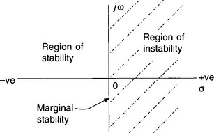
Figure 3.5
In a similar way, we can represent discrete signals and systems by their p–z diagrams in the z-plane. For example, if a discrete signal has a z-transform, X(z), given by:
then there will be a zero at 0.2 and, as the denominator factorizes to (z + 0.3 ± j0.2), complex conjugate poles at −0.3 ± j0.2. The p–z diagram is shown in Fig. 3.6.

Figure 3.6
We know that the locations of signal poles and zeros in the s-plane give us a good idea of the signal shape – but how do we interpret these positions in the z-plane? Also, which regions in the z-plane correspond to stability and instability?
To answer these questions we need to start with the link between the s-plane and the z-plane. Although we have used the z−n operator, and appreciate that it indicates a delay of n sampling periods, no mention has yet been made of any link between z and s. In fact there is a relationship between them and it is an extremely important one. This is given by:
where T is the sampling period. (Just accept this relationship for now – it will be explained later in the chapter.)
Using this relationship we will first consider the issue of stability.
3.7 STABILITY AND THE z-PLANE
We know that the imaginary axis in the s-plane is the boundary between the areas of stability and instability and that this boundary is defined by s = jω. From z = esT, this boundary must therefore map on to the z-plane as:
In other words, this equation defines the boundary between the stable and unstable regions in the z-plane.
O.K. – but what does this boundary look like? In fact, the equation z = ejωt defines a circle, centred on the origin, and with a radius of 1.
This is far from obvious and, to prove it, we need to use Euler’s identity. This tells us that:
It follows that we can rewrite z = ejωt as:
Figure 3.7 shows the point representing this z-value, plotted on the Argand diagram.

Figure 3.7
From the theory of complex numbers, or just from Fig. 3.7, the length of Az must be given by ![]() which is equal to 1, i.e.
which is equal to 1, i.e.
Also, the tan of the angle made by Az with the real, positive axis is given by
and so this angle must be ωT.
From Fig. 3.7 it should be clear that these magnitude and angle values do indeed define a unit circle in the z-plane, with its centre at the origin. This is because the length of the line Az, from the origin to the z-value, is always 1, and it makes an angle of ωT with the positive real axis. Therefore, as the signal frequency increases, i.e. as ω gets larger, z must mark out a circle of radius 1.
So we now know that the imaginary axis in the s-plane transforms to this ‘unit circle’ in the z-plane, i.e. this circle is the boundary between the stable and unstable regions in the z-plane. This leaves just one obvious question to be answered: ‘Is the stable region inside or outside the circle?’ The easiest way to decide on this is to map an ‘unstable’ pole in the s-plane, onto the z-plane, and see where it lies. Any positive s-value corresponds to a point on the unstable right-hand half of the s-plane. As s = 0 corresponds to a z-value of 1 (e0 = 1), any positive s-value must therefore transform to a z-value which is greater than 1 – i.e. to a point outside the unit circle.
It follows that, for the z-plane, it is the area outside the unit circle which is the region of instability and the area enclosed by the circle the region of stability – the unit circle itself corresponds to marginal stability (as does the imaginary axis in the s-plane).
These important ‘s-to-z’ mappings are summarized in Fig. 3.8.

Figure 3.8
3.8 DISCRETE SIGNALS AND THE z-PLANE
We now know that the area outside the unit circle in the z-plane corresponds to the right-hand half of the s-plane. In other words, if the z-domain transfer function of a discrete system has a pole outside the unit circle in the z-plane, then this is an unstable system. It also means that if the z-transform of a discrete signal has a pole in this area, then the signal amplitude increases with time.
But how, exactly, is the shape of the discrete signal related to its z-plane, pole–zero diagram? To answer this question, we need to start with an s-plane pole of a continuous signal. We know that the position of an s-plane pole can be expressed, completely generally, as s = σ + jω.
So, from z = esT, an s-plane pole will map to the z-plane as:
We now need to look, in more detail, at the two exponential expressions, eσT and ejωT, that make up z.
From earlier work we know that we can replace the ejωT part by cos ωT + j sin ωT (Euler’s identity), i.e. it indicates a point that is unit distance from the origin. Further, the line joining this point to the origin makes an angle of ωT with the positive real axis.
The ‘eσT‘ part is real, and so just corresponds to a real number. For example, if T = 0.1 s and σ = −2, then eσT ≈ 0.82. This part therefore acts as a multiplier and must fix the distance from the pole to the origin (Fig. 3.9). The line joining the pole to the origin is usually referred to as the pole vector. We know that, for continuous signals, σ indicates how rapidly the signal decays or increases. It therefore seems reasonable that the more negative is σ, i.e. the shorter the distance from the pole to the origin, the more rapidly the discrete signal decays.
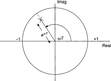
Figure 3.9
To summarize, it is the angle made by the pole vector with the positive real axis that represents the signal frequency, while the length of the vector tells us how quickly the signal is decaying or increasing – the shorter the vector the more rapid the decay rate.
To make this clearer, let’s imagine that we have a discrete signal that has a z-transform of l/(z − 0.5). The simple p–z diagram is shown in Fig. 3.10.

Figure 3.10
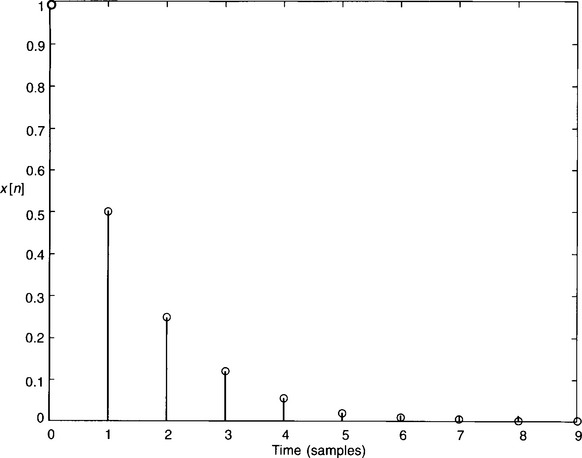
As the pole vector from the pole to the origin makes an angle of zero with the positive real axis, then this must represent a discrete signal of frequency 0 Hz, i.e. a d.c. signal. Also, as the pole vector has a length of 0.5, then this indicates that the signal should fall to a half of its previous value every sampling period.Figure 3.11 is the MATLAB plot for this signal – encouragingly it agrees with our prediction.
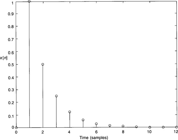
Figure 3.11
To confirm this plot we can simply carry out the division of 1/(z − 0.5). This gives z−1 + 0.5z−2 + 0.25z−3 + 0.125z−4 + …, which agrees with the MATLAB plot.
Notice that, although it has the expected rate of decay, the signal is delayed by one sample period, i.e. it starts at t = T and not t = 0. This is not immediately obvious from the p–z diagram, but is predicted by the long division.
This was a fairly simple example, having real roots, but what if the signal z-transform had been something more complicated, such as 1/(z2 – z + 0.5)?
As the denominator has the complex conjugate roots of 0.5 ± j0.5, then the p–z diagram is as shown in Fig. 3.12. The pole vector angle is 45° (and so ωT = 45° or π/4 rad. (N.B. It is the angle made by the pole vector in the top half of the z-plane which is important, i.e. 45° rather than the 315° or −45° in the bottom half.)
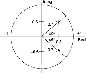
Figure 3.12
If we use a sampling period of 0.1s then this gives:
or ω = 2.5π rad/s, which is equivalent to a frequency of 1.25 Hz, as ω = 2πf.
The pole vector has a length of 0.7, and so we would expect the discrete signal to be a decaying sinusoid of frequency 1.25 Hz, the sinusoid decaying by a factor of 0.7 every 0.1 s.
The MATLAB plot, Fig. 3.13, certainly confirms the signal frequency, i.e. it has a period of 0.8 s and so a frequency of 1.25 Hz. It also agrees with the expected rate of decay – although the latter is not quite so easy to identify. Again note the delay of one sample period.

Figure 3.13
N.B. If the pole-pair (or single pole if d.c.) lies on the unit circle, then this corresponds to an undamped signal, i.e. one with a constant amplitude, while poles outside the unit circle correspond to a signal of increasing amplitude. For example, if the length of the pole vector is 1.2, then the signal increases by a factor of 1.2 for each sample period. This signal could be a d.c. signal or sinusoidal. Obviously, if the signal is sinusoidal then this increase is superimposed on to the normal sine variation, as is a decay for poles inside the unit circle.
3.9 ZEROS
You will remember that signal zeros in the s-plane do not change the overall shape of the signal but they do affect the magnitude – the nearer a zero is to a pole, the less the size of the corresponding signal component. Zeros have a similar effect in the z-plane but here they also affect signal time delays. Earlier we looked at a signal with a z-transform of 1/(z − 0.5). This signal is a decaying d.c. waveform with a delay of one sample period (Fig. 3.11). What if the z-transform had been z/(z − 0.5)? The only difference with this signal is that it has a zero at the origin. The corresponding signal is shown in Fig. 3.14. Note that there is now no time delay, i.e. the effect of the zero at the origin is to eliminate the time delay of one sampling period. This can easily be confirmed by dividing z by (z − 0.5) which gives 1 + 0.5z−1 + 0.25z−2 + … rather than z−1 + 0.5z−2 + 0.25z−3 + …. So the very existence of the zero will get rid of this time delay. Further, if the zero had not been at the origin, its closeness to the pole would also have affected the signal size. For example, Fig. 3.15 shows the signal corresponding to a z-transform of (z − 0.2)/(z − 0.5), i.e. the presence of this zero results in a greater rate of decay between the first and second samples – the closer the zero to the pole, the greater will be the reduction. Again, there is no delay.

N.B. MATLAB p–z diagrams are obtained using the ‘z-plane’ function. For example:
![]()
was used to produce the p–z plot of Fig. 3.15. Displaying more than one plot at the same time, i.e. the p–z plot and the corresponding signal, can be achieved by using the MATLAB ‘subplot’ function. Refer to the user manual for further details.
3.10 THE NYQUIST FREQUENCY
Consider a discrete signal represented by a pole on the negative real axis. For example, let the signal z-transform be given by X(z) = 1/(z + 0.5). This signal will have a z-plane pole at −0.5 and so the pole vector angle is 180° or π radians (Fig. 3.16).

Figure 3.16
Let’s assume a sampling frequency of 10 Hz, i.e. T = 0.1 s. As the phase angle (θ) = ωT, then π = 0.1 ω and so this pole indicates a signal with angular frequency of 10π, or f = 5 Hz.
Note that this frequency is half the sampling frequency of 10 Hz, i.e. it is the Nyquist frequency – the maximum signal frequency if aliasing is to be avoided. This is not just a coincidence but will always be the case, no matter what the sampling frequency.
A signal represented by a pole on the negative real axis has a frequency equal to the Nyquist frequency.
3.11 SELF-ASSESSMENT TEST
1. Sketch the signal represented by the p–z diagram shown in Fig. 3.17, by inspection of the diagram only. Then check your prediction by carrying out a suitable polynomial division.

Figure 3.17
2. Each of the poles/pole-pairs shown in Fig. 3.18 represents a separate discrete signal. Given that the sampling frequency is 120 Hz, state the frequencies of each of the signals.

Figure 3.18
3. Map the poles/pole-pairs shown on the s-plane diagram of Fig. 3.19, onto a z-plane diagram, assuming a sampling frequency of 2 Hz. (N.B z = esT.)

Figure 3.19
3.12 THE RELATIONSHIP BETWEEN THE LAPLACE AND z-TRANSFORM
Earlier, I promised to show where the vital relationship z = esT comes from – well this is it!
To be able to do this, we first need to go back to the definition of the Laplace transform, X(s), for a continuous signal, x(t), i.e.

The discrete version of this signal, i.e. the signal sampled every T seconds, will only exist at time = 0, T, 2T, 3T, etc. It follows that we first need to replace t with nT, where n is 0, 1, 2, 3 ….
Also, the integral sign, which indicates the area under the x(t) plot, has no meaning when dealing with discrete signals, as they consist of infinitesimally thin pulses. The equivalent process is the addition of the pulse magnitudes and so we must replace the integral symbol with the summation symbol.
The Laplace transform then becomes:
where X* indicates the discrete version of the Laplace transform.
If we now define the operator z as:
which you should recognize as the definition of the z-transform.
In other words, it is this particular relationship of z = esT which causes the z-transform to emerge from the Laplace transform.
3.13 RECAP
• The z-plane plays a similar role in the design and analysis of discrete systems to that of the s-plane in the design and analysis of continuous systems.
• Points on the s-plane map on to the z-plane as z = esT.
• Signals represented by poles within, on and outside the z-plane unit circle are decaying, non-decaying and increasing in amplitude respectively.
• The frequency of a discrete signal is obtained from the angle made by the pole vector with the positive real axis, while the vector magnitude indicates the rate of decay – the shorter the vector the greater the rate of decay. A selection of p–z diagrams along with the corresponding signals is shown in Fig. 3.20.

Figure 3.20
3.14 THE FREQUENCY RESPONSE OF CONTINUOUS SYSTEMS
We have come this far through a book on digital signal processing – which is largely to do with digital filters – and there has been no mention made of frequency response, even though the concept of frequency response is pretty fundamental to filter analysis and design! I assure you that this has not been an oversight on my part. It is just that we are only now in a position to make much sense of the frequency response of discrete systems.
Before we look at this very important topic it’s best to take a step backwards, and first remind ourselves of how we can find the frequency response of continuous systems. We will also look at how we can get this information from s-plane p–z diagrams.
The frequency response of a system is the way in which the gain of the system, and also the phase difference between the output and input signals, depend on the signal frequency. The test signal is always a non-decaying, pure sinusoidal waveform.
Suppose we have an analogue system with a transfer function given by T(s) = (s + 1)/(s + 2), and we need to find its frequency response. We know that s is the complex frequency of a signal, i.e. s = σ + jω, where σ indicates the rate of decay of the signal and ω is its angular frequency. However, as we are only interested in the response to a test signal which is a non-decaying sine wave, then σ = 0 and so we can replace s with just jω.
To find the gain of the system we need to find the magnitude of this complex function, i.e.
To find the phase relationship between output and input we must get the phase angle of T(jω). From complex number theory, this phase angle is given by:
For example, let’s imagine that we are interested in the gain at an angular frequency of 1 rad/s. Substituting ω = 1 into equations (3.2) and (3.3) gives a gain of ![]() or 0.63 and a phase angle, ∠T(jω), of
or 0.63 and a phase angle, ∠T(jω), of ![]() , i.e.
, i.e.
You are probably very familiar with what we have just done, as this is the normal method used to find the frequency response of a system. However, there is an alternative way of doing this which makes use of the p–z diagram for the system. This method can often be more convenient, especially when we want to design or analyse filters.
To demonstrate this approach we will stick with the same system, i.e. T(s) = (s + 1)/(s + 2). First its p–z diagram must be drawn (Fig. 3.21). This is a particularly simple one, having a zero at −1 and a pole at −2.

Figure 3.21
The gain and phase angle at 1 rad/s will again be found – we can then check against the values obtained earlier, using the ‘traditional’ method. To do this, a point A needs to be placed at position (0 + j).
N.B. This point represents a non-decaying, sinusoidal signal of angular frequency 1 rad/s, (s = jω = j).
To get the gain of the system, all we need to do is find the distances from A to the zero and to the pole and then divide these two distances. The zero distance is ![]() and the pole distance is
and the pole distance is ![]() and so the gain is
and so the gain is ![]() which is what we got using the ‘normal’ method. This isn’t too surprising as, for any ω value, the length of the zero vector from the zero to A is exactly the same as the magnitude of the numerator of equation (3.2), i.e.
which is what we got using the ‘normal’ method. This isn’t too surprising as, for any ω value, the length of the zero vector from the zero to A is exactly the same as the magnitude of the numerator of equation (3.2), i.e. ![]() , while the length of the pole vector is the same as the magnitude of the denominator,
, while the length of the pole vector is the same as the magnitude of the denominator, ![]() .
.
To find the phase angle we just measure the angles between the positive real axis and both the zero vector and the pole vector, and then subtract these two angles. As the zero angle, θZ, is tan−11 (45°), and the pole angle, θp, is tan−1 1/2 (26.6°), then this gives a phase angle of 18.4° – exactly the same as we derived earlier using the other method.
This graphical method gives a general expression for the phase angle of tan−1 (ω/1) − tan−1 (ω/2), which, once again, is exactly the same as we obtained using the more traditional approach (equation (3.3)).
This graphical approach is very useful in that we can get a good idea of the frequency response just by inspection of the positions of the poles and zeros. For example, if a pole lies very near to the imaginary axis at ω = 3 rad/s say, then we would expect a large gain at this frequency, while if it had been a zero, then the gain will be low. With experience it is possible to place poles and zeros so as to design a filter with the required response – this is a particularly useful technique when designing digital filters.
Example 3.1
Find the gain and phase angle for the previous system, i.e. T(s) = (s + 1)/(s + 2), for angular frequencies of 0 rad/s (d.c), 2 rad/s and also for very large frequencies.
• ω = 0 rad/s: this frequency (d.c.) is represented by point A in Fig. 3.22.

Figure 3.22
• ω = 2 rad/s: this frequency is represented by point B:

• For large frequencies: here, both zero and pole distances will be very large and approximately the same size. It follows that the gain must become very close to unity. Similarly, both zero and pole angles will approach 90° for sufficiently large frequencies and so the phase angle will be approximately zero.
Armed with this information, it should be possible to make a reasonable stab at sketching the frequency response. Figure 3.23 shows precise MATLAB plots, produced using the ‘bode’ function, i.e.:

Figure 3.23

Remember that a Bode plot displays both the gain and the phase angle against log ω (or log f), the gain being in dB (20 log gain). So we are looking for gains of 20 log 0.5, 20 log 0.63, 20 log 0.8 and 20 log 1 at angular frequencies of 0, 1 and 2 rad/s and very large frequencies respectively, i.e. approximately −6 dB, −4 dB, −1.94 dB and 0 dB. Our predicted gain and phase values agree closely with the Bode plot values. Note that it is impossible to display 0 rad/s on a log scale. However, our gain has clearly settled at −6 dB by 0.1 rad/s and the phase angle appears to be approaching 0.
N.B. In this particular example we only had one pole and one zero. For the more general case, where there are several zeros and poles:

where k is the ‘pure’ gain in the system. For example, if the transfer function of the system had been 3(s + 1)/(s + 2), then k = 3.
‘П’ is the shorthand symbol commonly used to represent ‘product of, in the same way as ‘Σ’ is used to indicate the sum.
If there is no zero, e.g. T(s) = 1/(s + 2), then a ‘1’ must be used for the zero distance.
3.15 SELF-ASSESSMENT TEST
A continuous system has a transfer function given by T(s) = 4(s + 1)(s + 2)/(s2 + 2s + 2). Plot its p–z diagram and use this diagram to find the response, both gain and phase, at 0, 1 and 2 rad/s and also for very large frequencies. Also, sketch the complete frequency response.
3.16 THE FREQUENCY RESPONSE OF DISCRETE SYSTEMS
As with continuous systems, the frequency response of a discrete system can also be found from its pole–zero diagram. However, as it is the unit circle in the z-plane that corresponds to the imaginary axis in the s-plane, here the ‘frequency point’ moves around the unit circle in an anticlockwise direction as the signal frequency increases. The point starts at z = +1 (d.c), and ends at z = −1 (the Nyquist frequency).
For example, say we have a discrete system with a transfer function given by T(z) = (z + 1)/(z − 0.5), and we need to find the response at d.c. (0 Hz), 1 Hz and 2 Hz, given that the sampling frequency is 8 Hz.
The p–z diagram is shown in Fig. 3.24. As the sampling frequency is 8 Hz, the Nyquist frequency is 4 Hz, and so the three frequencies of 0, 1 Hz and 2 Hz must correspond to points A, B and C respectively.

Figure 3.24

Phase angle = Σ zero angles – Σ pole angles
• Frequency = 1 Hz: The pole and zero distances are more difficult to calculate here – using a scale diagram and measuring the distances is an alternative approach. However, whichever method is used, the zero distance, BZ, ≈ 1.84 and the pole distance, BP, ≈ 0.73. Check these for yourself.
Also the zero angle ≈ tan−1(0.7/1.7) = 22.3° and the pole angle ≈ tan−1 (0.7/0.2) = 74.1°.
• Frequency = 2 Hz: Here the zero distance is √2 and the pole distance is ![]() (Fig. 3.25).
(Fig. 3.25).

Figure 3.25
The zero angle is 45°, and the pole angle is {180° − tan−1(l/0.5) = 116.5°}.
N.B. Remember that the phase angle is always measured between the horizontal, pointing to the right, and the vector, measured from the horizontal to the vector moving in an anticlockwise direction.
Figure 3.26 shows the MATLAB frequency response plots for the system, drawn using the ‘freqz’ function. Note that with the ‘freqz’ function the frequency axis is linear and also ‘normalized’, i.e. the frequency of ‘1’ corresponds to the Nyquist frequency.
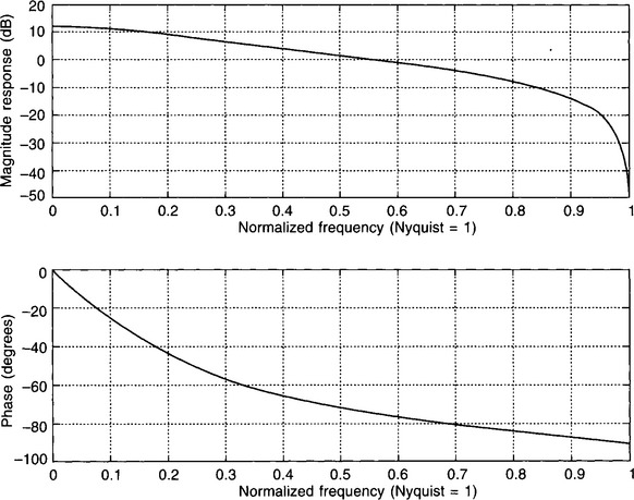
Figure 3.26
Our gain values agree very well with the magnitude plot of Fig. 3.26, i.e. at 0 Hz, 1 Hz (0.25fN) and 2 Hz (0.5fN), we get gains of 4, 2.5 and 1.27 respectively, or 12 dB, 8 dB and 2 dB. Our corresponding phase angles of 0, −51.8°, and −71.5° are also in good agreement.
The program used to produce these plots is:

N.B. Because the frequency axes of the plots generated by the ‘freqz’ function are linear rather than logarithmic, these plots are not strictly Bode plots. There is a MATLAB Bode plotting function for discrete systems, which could have been used. This is the ‘dbode’ function. This alternative display (Fig. 3.27) was produced using:

Figure 3.27

However, this function is not ideal as the gain is shown as becoming very low at the Nyquist angular frequency of approximately 25 rad/s. Because of this huge magnitude range, values of interest are extremely compressed. This problem can be overcome to some extent but, generally, the ‘freqz’ function is much more convenient.
Notice that the frequency response is only displayed up to the Nyquist frequency on both of the freqz and the dbode plots. The response does not stop at this frequency, of course, but continues from fN to fs, i.e. as the frequency point proceeds around the unit circle. Due to the symmetry of the p–z diagram about the real axis, this portion of the magnitude response is a mirror image of that up to fN. The frequency response then repeats itself as the frequency point makes a second revolution of the unit circle, corresponding to frequencies from fs to 2fs – and so on. However, you need to be clear that this is the frequency response of the digital processor at the heart of the DSP system. The output from the complete system will only contain signal components with frequencies up to fN. This is because the reconstruction filter at the output of the DSP system is a lowpass filter, with a cut-off frequency of fN (see ‘The reconstruction filter’, Section 1.4). For this reason we have little interest in the frequency response above the Nyquist frequency.
Alternative calculation of frequency response
As an alternative to using the p–z diagram, the frequency response of a continuous system can be calculated directly from its transfer function by replacing s with jω. We can also calculate the frequency response of a discrete system directly from its transfer function but, as usual, it’s a bit more complicated.
As an example, let’s take the system considered earlier in this section, i.e. the one with the transfer function (z + 1)/(z − 0.5) and with T = 0.125 s.
We first need to move from the z-domain to the s-domain using the link provided by z = esT. However, as we are interested in the frequency response, then s = jω, and so we need to replace z with ejωT.
Substituting this z-value into the transfer function gives
This expression doesn’t look too hopeful! However, we can improve things by applying Euler’s identity, i.e. ejθ = cos θ + j sin θ. This gives
which allows the gain and phase angle to be obtained from ω = 0 to ω = π/T (the Nyquist angular frequency).
For example, if we want the response at 1 Hz (2π rad/s) say, then as T = 0.125 s:
which has a more familiar format.
and
N.B. Before moving on, it would be worth using this method to also check the frequency response at 0 and 2 Hz for yourself.
Example 3.2
A digital filter has a transfer function of 3(z − 0.5)(z + 1)/(z2 + 0.25). Find the frequency response at 0 Hz, and 2.5 Hz, (a) by using the p–z diagram and (b) directly from the transfer function. The sampling frequency is 10 Hz.
• This system has zeros at 0.5 and −1 and poles at ± j0.5. The p–z diagram is shown in Fig. 3.28.

Figure 3.28

Phase angle = Σ zero angles – Σ pole angles
• f = 2.5 Hz: from Fig. 3.29,

Figure 3.29

(b) Directly from the transfer function.
• f = 0 Hz: from z = ejωT, with ω = 0, we get z = 1. (We didn’t really need to use z = ejωT to find that z = 1 corresponds to 0 Hz.)
Substituting z = 1 into the transfer function:
This is a real function and so gain = 2.4 and phase angle = 0 (as the imaginary component is zero).
• f = 2.5 Hz: ω = 2πf = 5π rad/s. We could use z = ejωT to find the z-value corresponding to this particular frequency, but this is another frequency where we don’t have to bother as it’s obvious that, as 2.5 Hz is a half of the Nyquist frequency, z = j.
Substituting z = j into the transfer function:

(N.B. The denominator of −0.75 can be thought of as −0.75 + j0, giving a phase angle of 180°.)
3.17 UNSTABLE SYSTEMS
Don’t forget that discrete systems with transfer function poles outside the unit circle are unstable, and so must be redesigned. Figure 3.30(a) shows the unit step response for a system with a pole at 1.2, while Fig. 3.30(b) is the unit step response for a filter with conjugate poles at 0.8 ± j0.8, again, outside the unit circle. More work on these particular designs is clearly needed!
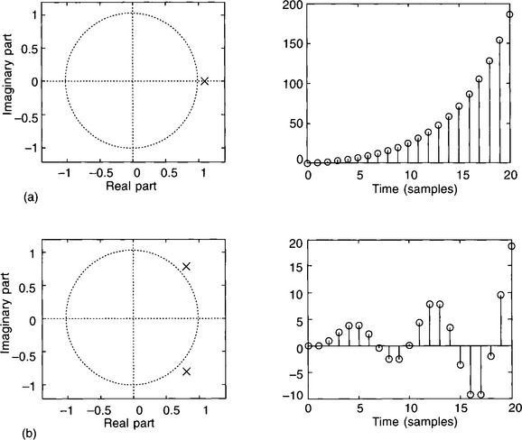
Figure 3.30
3.18 SELF-ASSESSMENT TEST
A digital filter has a transfer function given by
The sampling frequency is 16 Hz.
3.19 RECAP
• The frequency response of a continuous system can be found by replacing swith jω in the transfer function and, for a discrete system, by replacing z with ejωT.
• The frequency response can also be found from the transfer function p–z diagrams using
and
• The frequency point moves up the imaginary axis from the origin (d.c.) for continuous systems and around the unit circle in an anticlockwise direction from z = 1 (d.c.) to z = −1 (the Nyquist frequency) for discrete systems.
3.20 CHAPTER SUMMARY
We started this chapter by looking at the s-plane – i.e. by reviewing how continuous signals and systems can be analysed from their pole–zero diagrams. We then moved to the z-plane, which serves the equivalent purpose for discrete systems and signals. The link between the s- and z-planes was shown to be provided by z = esT.
The regions in the z-plane corresponding to stability, marginal stability and instability were identified as being within the unit circle, on the unit circle and outside the unit circle respectively.
The shapes of discrete signals were established from the positions of their poles and zeros – the general shape being determined by the pole positions, while the zero positions govern the magnitude of the signals. The presence or otherwise of signal zeros also controls signal delays.
The frequency response of a discrete system was derived directly from the z-plane transfer function by using z = ejωT = cos ωT + j sin ωT. The frequency response was also obtained from the p–z diagram of the system transfer function using
and
This chapter has been mainly concerned with the analysis of discrete systems but you have now also acquired many of the tools needed to design digital systems.
3.21 PROBLEMS
N.B. If you have access to MATLAB then use it wherever possible to check your answers to the following problems.
1. A filter has a transfer function of T(z) = (z − 0.1)/(z − 0.3) and is used with a sampling frequency of 1 kHz.
(a) Sketch the pole–zero diagram for the filter.
(b) Use your pole–zero diagram to estimate the gain and phase angle at 0 Hz and 250 Hz.
(c) Check the gain and phase angle at 250 Hz directly from the transfer function. Also use this method to find the gain and phase angle at 375 Hz.
2. A continuous filter has a transfer function, T(s), given by T(s) = (s + 2)/[(s + 1)(s + 3)].
(a) Design a digital filter that has equivalent poles and zeros by making use of the relationship z = esT. The sampling frequency is 10 Hz.
(b) Compare the d.c. gains of the two filters either with the aid of their p–z diagram or directly from their transfer functions. Comment on these values.
3. A digital filter has the z-domain transfer function of l/(z2 − z + 0.5). Sketch the p–z diagrams for the filter outputs when the input is (a) a unit sample sequence and (b) a discrete unit step. Use the system p–z diagram to find the gain of the system at 0 Hz and also at fs/4, where fs is the sampling frequency.
4. By using the function z2/(z + 1) as an example, explain why it is impossible for a system transfer function to have more zeros than poles. (Hint: Consider the response of the system to a unit sample sequence.)
5. A digital filter has a transfer function of the form T(z) = (z2 + 0.81)/(z2 + p2). The filter is to have a minimum gain of −6 dB occurring at a frequency of 50 Hz. Given that the sampling frequency is 200 Hz, find the appropriate p-value. (Hint: First sketch a p–z diagram to show the zero positions.) Also find the gain at 0 and 100 Hz. Hence sketch the magnitude response of the filter.