
SIGNAL CAPTURE
4.1 Introduction
In the last chapter, we looked at the fundamental concepts for generating signal information that will be presented to the DUT input. In this chapter, you’ll learn how to use those same concepts and equations to capture the DUT signal output. A mixed signal device may generate analog information in either analog or digital form, which in turn is captured by the ATE systems’ signal capture instruments. The signal capture instruments store a numerical replica of the analog information from the DUT in the test systems’ capture memory.
If the stimulus waveform is in analog form, the signal capture uses an analog-to-digital converter to create a numeric sample set that represents the original signal data.
The input of the ADC is filtered to remove spurious high-frequency noise, and amplified to the specified range. If the stimulus waveform is in digital form, the signal capture receives the data from the digital pin receivers. The level and timing parameters are the same as for a digital test. Even if the data from the DUT is in digital form, it represents analog information, not a logic function.
The contents of the signal capture memory represent a digitized analog signal, not digital logic states. Instead of comparing the captured digitized signal with a pattern, the signal data is analyzed by a digital signal processor (DSP). The DSP analyzes the signal data to extract analog signal information, such as peak, RMS, signal-to-noise, and harmonic distortion.
In most ATE systems, the signal capture can be started and stopped through either the program or micro-code in the pattern—just like the source.

4.2 Digital Signal Capture Hardware
During a digital capture, the output signals from the DUT are compared against the programmed VOL and VOH levels of the test system’s per-pin receiver circuit. The pin receiver outputs indicate if the device signal was a valid logic high (above VOH), a valid logic low (below VOL), or an in-between state (Hi-Z).
For a logic test, timing information selected by the sequencer is sent to the format and timing section, which generates a strobe to the compare circuit. The strobe triggers the compare circuit to compare the DUT logic state with the expected data state described in the pattern vector. In a mixed signal test system, the strobe edge latches the DUT output logic state into the capture memory.
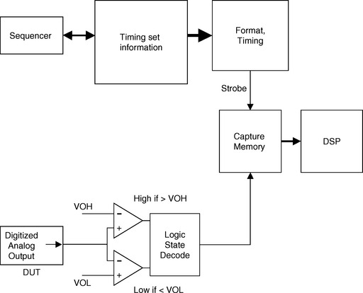
Example: If the device under test is an ADC, the output will be in digital form, and will be captured with the digital instrumentation.
4.3 Analog Signal Capture Hardware
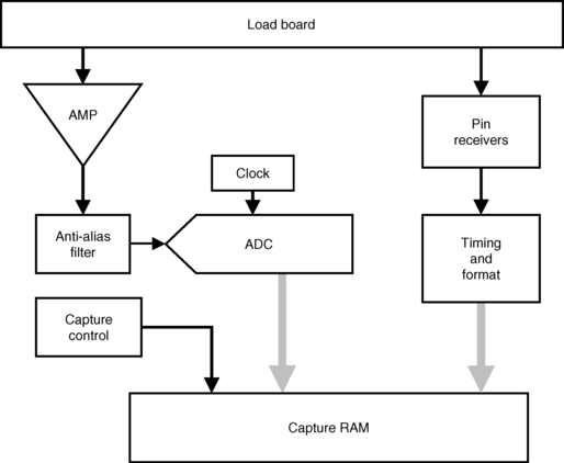
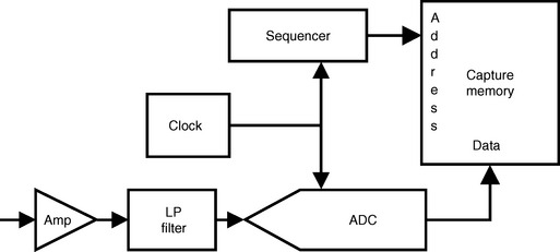
The purpose of the analog signal capture is to digitize and store the analog signal generated by the DUT for analysis by the DSP unit. The amplifier provides a ranging function. The programmable gain amplifier matches the amplitude of the signal with the fixed range of the ADC. The anti-alias filter rejects spurious high-frequency information before it is digitized. Unwanted high-frequency components can significantly degrade the quality of the signal analysis. Signal information that has been filtered and amplified is digitized by ADC, controlled by the capture clock. The conversion speed and amplitude resolution of the ADC characterize the target application of the analog signal capture. The analog signal capture sequencer is controlled by the ATE system software to store a sequential sample set in the capture memory. The rate at which the sequencer loads data into the capture memory is also controlled by the capture clock. To store the DUT signal, a sequence of numeric data points from the ADC is stored in the capture memory. Typical ATE signal capture units have a capture memory from 256 K to 1 MB deep by 20 bits wides.
4.4 The Digitizing Process
Digitizing an analog signal represents a continuous signal with a series of discrete numeric values. Each value is called a sample. To digitize means to sample and quantify. This implies that not all data points on the continuous signal are captured. Digitizing attempts to represent a continuous signal with a series of discrete steps. The process of converting from analog to digital has several inherent constraints.
4.4.1 Quantizing Error
Quantizing error is non-random noise of fixed value that is caused by the uncertainty of the digitizing process. A simple two-bit ADC illustrates quantizing error. If the sampled analog value is between two digital levels, the uncertainty is expressed as quantizing error. What happens when the input signal does not correspond exactly to one of the threshold combinations? If the input signal level was at 2.5 volts, for example, the ADC would generate either a 11 or 10 code; and both cases would be in error. (And no, we don’t get to have a 11 and a half.) We’re stuck between bits.

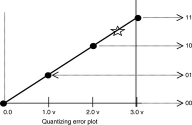
4.4.2 Quantizing Error and the LSB
If we divide the full range of the analog input by the total number of available digital codes, we can derive the smallest analog step size that can be represented by a unique digital code. Because this is equivalent to the Least Significant Bit of the digital code, it is called the LSB value. Quantizing error is the uncertainty “between bits.”
The worst-case quantizing error occurs when the signal value is exactly between two code thresholds and is never more than one-half of the LSB value.
Consider a 4-bit ADC, with a 1.5-volt full-scale input range and 100-mV steps. An input level of 0.4 volts will cause the ADC to generate an output code of 0100. What will be the output code if the input level is 0.41 volts? How about 0.42 volts? You see the problem, eh? That’s quantizing error.
Table 4.2
| Input Level | Output Code |
| 1.5 | 1111 |
| 1.4 | 1110 |
| 1.3 | 1101 |
| 1.2 | 1100 |
| 1.1 | 1011 |
| 1.0 | 1010 |
| 0.9 | 1001 |
| 0.8 | 1000 |
| 0.7 | 0111 |
| 0.6 | 0110 |
| 0.5 | 0101 |
| 0.4 | 0100 |
| 0.3 | 0011 |
| 0.2 | 0010 |
| 0.1 | 0001 |
| 0.0 | 0000 |
The moral of the story is that the tester will lie to you. It can’t help it. When we try to capture a signal, the tester will process the signal based on the acquired data, but we should not expect the acquired data to exactly match the signal. The error introduced by the digitizer process usually looks like noise. Even if the signal from the DUT is perfectly pure, the tester will actually add noise, because of the quantizing error.
4.4.3 Digitizer Resolution
Because quantizing error is related to the LSB value, the range and resolution of the digitizer’s analog-to-digital converter directly affects the amount of quantizing error. What will be the quantizing error for ADCs of different resolution with 5.0-volt signal?
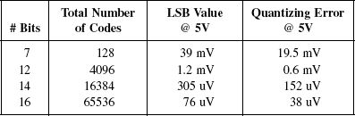
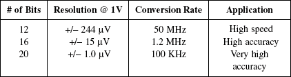
With a 5-volt range on a 16-bit capture instrument, the uncertainty is no more than 38 uV; a precision of 500 times greater than a 7-bit capture instrument.
Example
When using a 16-bit capture instrument on a 5-volt range, the instrument returns a reading of 38 uV. This may or may not be the same as the actual signal level. Because of the limitations of the digitizer, the actual level could be anywhere from 0 volts to 76 uV—there is no way to tell without improving the instrument resolution.
4.4.4 Sample Size and Sample Rate
The purpose of digitizing a signal is to construct a sample set that represents the signal amplitude over time. The continuous analog data must be sampled at discrete intervals that must be carefully chosen to ensure an accurate representation of the original analog signal. The sample frequency is the rate at which the digitizer samples the input signal for conversion to a set of discrete numeric values.
Ideally, the greater the number of samples (i.e., the higher the sample rate) that can be taken for any given signal duration, the greater the accuracy of the digital representation. However, acquiring many samples may take longer than acquiring fewer samples. Processing many samples usually takes longer than processing fewer samples. The constraints of the digitizer limit the sample frequency. The practical rule is to digitize the signal with as few samples as possible, but no fewer.
4.5 Nyquist and Shannon—Theoretical Limits
Nyquist’s Sampling Limit—The sampling frequency must be greater than twice the bandwidth of the signal.
Shannon’s Theorem—If a signal over a given period of time contains no frequency components greater than fx, then all of the needed information can be captured with a sample rate of 2 × fx.
4.5.1 Applications of Nyquist and Shannon
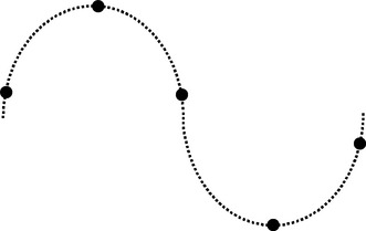
If a test program is designed to test a specific range of frequencies, the minimum sample rate may be only slightly greater than twice the bandwidth of the signal. The signal information can be completely determined if this condition is met. For capturing periodic signal information, just one extra sample is sufficient. At it turns out, the phase of the signal relative to the beginning and end of the capture sequence does not affect the quality of the data set. If there is an unknown phase shift in the DUT or the instrumentation, this does not prevent measuring the magnitude and frequency of the captured signal.
The underlying assumption in both Shannon’s Theorem and Nyquist’s Limit is that the sampling rate is consistent. That is, the sample period must be without variation across the sampling set. An average sample rate of 2 × fb does not meet the minimum conditions.
When testing for noise and distortion, estimating the actual signal bandwidth requires careful attention. A 1-kHz sine wave, for example, could theoretically be captured with a sample rate of 2.01 kHz. Applying Shannon’s theorem, however, it becomes clear that the only data to be completely captured will be less than 1.005 kHz (fs/2). This would collect no information about the harmonics or noise above 1.005 kHz.
Example
To calculate the actual minimum sample rate requires understanding the actual signal bandwidth, including distortion and noise. What would be the minimum sample rate to properly capture the following signal data?
• Test signal is 10.000 kHz sine wave
• Test for total harmonic distortion (THD) includes the 2nd and 3rd harmonics
Even though the primary signal is 10.0 kHz, the actual bandwidth of interest extends to 50.0 kHz. In that case, the sample frequency must be greater than 100 kHz, or twice the bandwidth of interest.
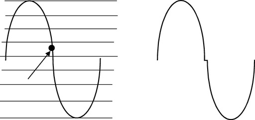
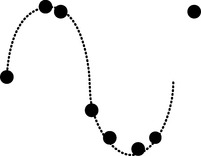
4.5.2 Signal Aliasing
What happens if Shannon’s Theorem is not met? What happens if the test program samples a signal at less than twice the signal frequency?
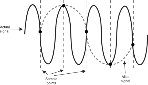
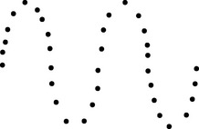
Big trouble! If the test program captures fewer than two samples per signal cycle, a false representation of the signal is generated from the available data points. If we view only the sample point from the preceding diagram, it appears as though the signal is of much lower frequency than the actual data. The test application can only interpolate based on the available data points.
The false signal is known as an alias. This error appears in both the time domain and the frequency domain. The purpose of the anti-alias filter in the capture hardware is to remove high-frequency signals that could cause an alias.
4.5.3 The Anti-Alias Filter
The roll-off characteristics of the anti-alias filter play a part in calculating the correct sample rate. A typical anti-alias filter in a signal capture unit may be configured as a selectable bank of filters. Each filter has a specified pass-band, and a roll-off characteristic.
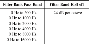
The roll-off specification indicates that signal frequencies above the pass-band will be rejected by 24 dB for every doubling of the signal frequency. Selecting the 0-1000-Hz filter will pass all frequencies within that range. Frequency components above the pass-band would be attenuated as follows:
| Spurious Signal Frequency | Attenuation |
| 2 kHz | −24 dB |
| 4 kHz | −48 dB |
| 8 kHz | −72 dB |
| 16 kHz | −96 dB |
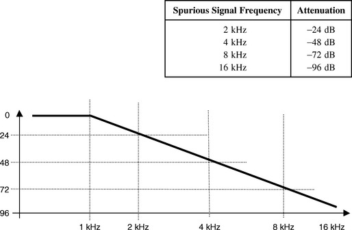
If you wanted to make sure that all signal components above the Nyquist point were attenuated by at least 96 dB, the sampling rate would need to be 32 kHz. You must program the sample clock at a high enough frequency to place the Nyquist point at a usable point on the filter slope. It’s a lot like what we went through with the reconstruction filter. First, you need to understand the filter response, then you need to calculate the sample frequency that will cause the Nyquist point to intercept the filter slope.
Filter Selection Example
Suppose you selected the 1-kHz band pass anti-alias filter. This would set up the capture hardware to accept all signal frequencies below 1 kHz, and to reject signal frequencies about 1 kHz. If the capture instrument sample rate (fs) is programmed to 16 kHz, then the Nyquist frequency would be fs/2, or 8 kHz.
Note that the selected configuration of the anti-alias filter has an attenuation of only −72 dB at 8 kHz. This would create inadequate filtering of spurious high-frequency signal information, and could generate incorrect measurement results. In order to avoid false measurements due to signal information above Nyquist, the sample frequency (fs) must be high enough to place the Nyquist point (fs/2) in the filter reject region. In order to fully utilize the anti-alias filter, it is common practice to choose a sample frequency that is at least 16 to 32 times the signal bandwidth.
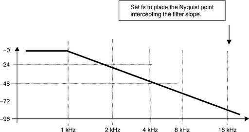
What Was That Again?
OK, it does seem a little backward, so let’s take another look. You want to make sure that you do not process any information above the Nyquist point, because of all the weird things that happen to the signal. But, we’re stuck with the filters that the ATE system gives us. If we had a super-deluxe filter with a 120-dB roll-off per octave, then we wouldn’t have to worry. Because the actual filter isn’t really all that steep, and it does not start to seriously kick in until three octaves (every octave doubles the frequency) above the pass-band, there’s only one thing left. We can’t change the target frequency, and we can’t change the filter roll-off—the only thing we can do is change the Nyquist point. By increasing the sample frequency, you can push the Nyquist point out to where it intersects the filter slope.
4.6 Sampling Rate and the Frequency Domain
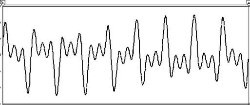
In the last section, we saw how a multi-tone waveform can be created by combining several sine waves of different frequencies. The result was a non-sinusoidal wave shape. As it turns out, any non-sinusoidal wave shape can be analyzed as a multi-tone, that is, as a signal made up of sine wave components. Frequency domain analysis deconstructs a signal into the sine wave components, and graphs the results according to magnitude across frequency.
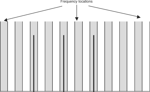
4.6.1 Frequency Resolution
The value of the base frequency (fbase) determines the step size in the frequency domain. In the time domain, the value of fi/fbase indicates the number of cycles in the sample set. In the frequency domain, the value of fi/fbase determines the signal location. Processing the digitized signal in the frequency domain requires that the digitizer sample rate and sample size is sufficient to produce the desired resolution. The fbase value is the step size, or x-axis resolution, in the frequency domain.![]()
Suppose that in order to test a captured signal for noise and distortion, you decide to measure the frequency domain energy at 100 Hz, 200 Hz, 300 Hz, 400 Hz, and 500 Hz. This means you need frequency domain data in increments of 100 Hz. To achieve a frequency resolution of 100 Hz, the sample size and sample rate must be selected to generate the corresponding fbase value.![]()
There’s no DSP magic that can bail you out here. The only way to establish the proper resolution in the frequency domain is to choose the correct sample rate and sample size in the time domain.
Example
In order to test a captured signal for noise, you decide to measure the frequency domain energy at 100 Hz, 200 Hz, 300 Hz, 400 Hz, and 500 Hz. You decide on a frequency resolution of 100 Hz in the frequency domain, but the test specification requires a sample frequency of 25.6 kHz. How many samples must be in your sample set to derive the required base frequency?
4.6.2 Resolution Trade-offs
You can evaluate the same signal with different levels of resolution in the frequency domain. The trade-off is the amount of information versus the required capture duration period. Because fbase is the reciprocal of the capture duration period, the lower the fbase value, the longer the required duration period. You could set up your sample rate and sample size to produce a frequency resolution of 1 Hz, but it’s going to cost you a full second of test time.
How much does one second of test time cost? Well, if you’ve working with a new tester platform, it could cost around 4 million dollars. By the time you factor in the amortization, interest, and utilization factors, the equipment cost works out to more than a million dollars per year. There’s about 31 million seconds in a year, so we’re looking at a tester cost of 3.3 cents per second.
Let’s look at one more example before we move on.
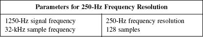
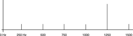
Result: The frequency domain data set will be arranged in steps of 250 Hz. That is, the frequency domain will show data at 0 Hz, 250 Hz, 500 Hz, 750 Hz, etc.
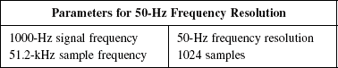
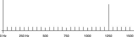
Result: The frequency domain data set will be arranged in steps of 50 Hz. That is, the frequency domain will show data at 0 Hz, 50 Hz, 100 Hz, 150 Hz, etc.
4.7 Capturing Periodic Sample Sets
Digitizing an analog signal has many of the same requirements as synthesizing a signal. Generating a useful data set for the analog signal source requires calculating the correct sample rate and sample size to produce an integer number of cycles. Acquiring a useful data set for the analog signal capture also requires calculating the correct sample rate and sample size to obtain a periodic sample set.
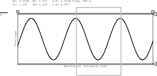
The sample window refers to the time period during which the digitizer is sampling the analog data, and is calculated by![]()
The window must be of the proper duration to correctly capture a periodic sample set of the analog signal. If the sample set duration is too long or too short, the captured signal data set will not properly represent the analog data.
Testing for frequency domain characteristics often requires the use of a computer algorithm called the Fast Fourier Transform (FFT). Once of the constraints of the FFT is that the input data will be processed as if it were periodic. The design of the FFT algorithm assumes that the data set can be duplicated without introducing signal error.
4.7.1 Application Example Overview
Let’s work through an example to illustrate the process for calculating capture instrument parameters.
OBJECTIVE: Determine the duration of the sample window that will capture an integer number of cycles for each frequency component of the analog signal.
PARAMETERS: The duration of the sample window is determined by the sample size and the sample rate.
PROCESS: Calculate the frequency resolution that divides evenly into all of the frequency components of the analog signal. Once the fbase has been determined, you can derive the proper sample size and sample rate.
Our objective is to calculate the sample size and sample rate for digitizing a multi-tone signal composed of 1680 Hz, 3750 Hz, and 5460 Hz.
4.7.2 The Largest Common Denominator
Step One: Remember that fbase is a periodic frequency, which represents the ratio of the sample frequency over the sample size. What is the periodic frequency, or fbase, that will divide evenly into all three components? (Find the largest common denominator.)
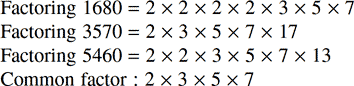
The largest common denominator is therefore 210 Hz, which we will select as the fbase. Recall that fbase is the reciprocal of the window duration.![]()
4.7.3 Verify Integer Number of Cycles
Step Two: Given an fbase frequency of 100 Hz, verify that the captured data set will contain an integer number of cycles for each component of the multi-tone.![]()
That is, the 4.7619-mS capture duration window will contain an integer number of cycles for each sine wave frequency of the multi-tone waveform.
4.7.4 Approximate fs and Sample Size
Step Three: Once you capture a periodic sample set of the multi-tone signal, you will perform a Fast Fourier Transform (FFT) to analyze the data in the frequency domain. The FFT transform requires that the sample set be a power of two, so you need to choose the number of samples and the sample rate to produce
We also know that the sample frequency should be at least 16 times the signal bandwidth, in order to make the best use of the anti-alias filter. As an approximation, we can therefore estimate the sample frequency as
Step Four: Applying DSP’s law, we can approximate the sample size from the preliminary sample frequency value, and the selected fbase value.![]()
The only problem is that the FFT requires a power of two sample size. That is, the FFT can process a sample size of 2, or 4, or 8, or 16; but it cannot process a sample set that is 5, or 14, or 18. Because the preliminary sample size of 416 samples is not a power of two, we must go through another iteration to determine the exact values for the sample frequency and sample size parameters.
4.7.5 Optimizing Capture Parameters
Step Five: We know the sample size must be greater than or equal to 416 samples to achieve the target capture parameters. To meet the FFT data set requirement, we must choose a sample size that is a power of two, and is also greater than 416. Recalculating with a sample size of 512 samples gives us the following:![]()
Step Six: As a proof, let’s apply the Golden Ratio to this application. Recall that the ratio of the sample frequency (fs) to the signal frequency (fi), is always the same as the ratio of the number of samples to the number of cycles.
4.8 Signal Averaging
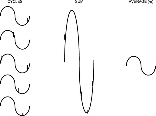
Signal averaging is a method for cancelling random noise in the captured signal data set. Over time, the value of Gaussian distribution noise averages to zero; so by taking an average of several signal cycles, the random noise error can be removed.
Consider five signal cycles, each with a random noise component. By summing the signal data and then generating an average, the random noise components are reduced by a factor equal to the square root of the number of averaged cycles. Because the signal information is periodic, the amplitude of the averaged data is unity for the signal. Because the noise components are non-periodic, the averaged data attentuates the noise information.
4.9 Capturing Unique Data Points
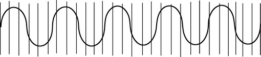
In general, most mixed signal test applications will return more complete results if the captured data is not redundant. For example, if the test program captures a 1.0-kHz signal using a sample rate of 16.0 kHz, each cycle of the signal will be represented by 16 consecutive samples. If the test program collects 5 cycles, it will have gathered the same 16 data points, relative to the signal cycle, 5 consecutive times.
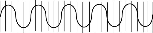
To collect new data for each cycle, the sample frequency and the signal frequency must be mutually prime. An integer ratio of fs/fi results in a redundant data set when capturing more than one cycle. A non-integer ratio of fs/fi allows each sample in the captured data set to represent a unique point of the captured signal.
This is one method for calculating the correct fs and sample size to ensure unique data points in the sample set.
4.9.1 Applications Example
Step One: The first iteration has the following parameters:
Relative to the signal, this will collect the same 16 data points for each cycle. In order to capture unique data points for each cycle, we need a second iteration of calculations.
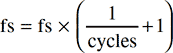
Step Two: Multiply fs by the reciprocal of the number of cycles +1.
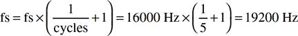
Calculate the new sample size:![]()
With these new parameters, the ratio of fs to fi is a non-integer, as is the number of samples per cycle.![]()
The number of signal cycles has not changed, only the number of samples per cycle. As a result, the capture duration, and therefore the signal acquisition time, is the same even though more information is being gathered.
4.9.2 Over-Sampling Technique
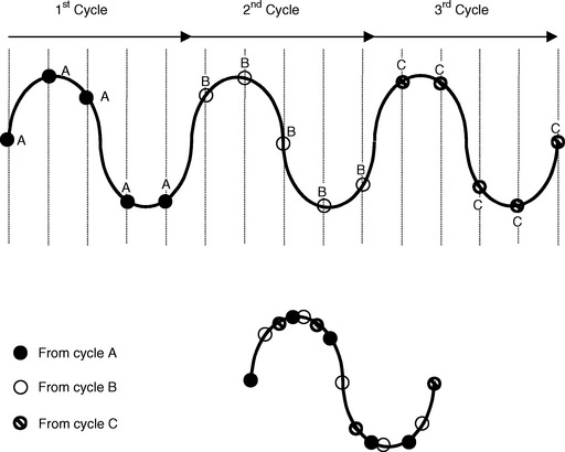
Another application of capturing unique sample points concerns a method known as over-sampling. In applications where the sample per cycle ratio is small, the digitizer can be programmed to capture unique points on the signal for each cycle. The end result is an effective sample rate, that is higher than the actual fs.
This technique is similar to that used in sampling scopes, where the signal is reconstructed on the basis of data collected under a large number of cycles. In order to properly reconstruct a signal from data collected under several cycles, the samples must take place at different points for each cycle, relative to the signal.
Consider the following scenario. You are developing a test program that includes a requirement to capture a 200.0-kHz signal at 10.0-MHz sample rate. The constraints of the ATE system capture instrumentation are such that the maximum sample clock (fs) is 1.0 MHz. If the test objective can be met by capturing data at 100-ns increments, or an effective 10.0-MHz capture rate, then over-sampling can provide a solution.
1. Calculate the period of the over-sampled fs.
Example: If you need an effective over-sample clock rate of 10 MHz, the period is 100 ns.
2. Add the over-sampled period to the actual sample period.
The actual sample clock is 1 MHz, which is equal to a period of 1000 ns. Adding the over-sample period gives 1100 ns, or a frequency of 909.0909… kHz. We can round this off to 909 kHz. This is your new actual fs.
3. Use the Golden Ratio to determine the new sample size and number of cycles.![]()
4. Capture unique data points across multiple cycles, and generate a composite data set.
By capturing a large number of samples over multiple cycles, the captured data can be reconstructed as a composite 100-nS sample set.
Note: A technique known as under-sampling is described in Chapter 5.
4.9.3 Over-Sampling Application Example
With a 200-kHz signal frequency and a 1.0-MHz sample clock, the digitizer will collect 5 samples for each cycle. By changing the sample clock frequency to 909 kHz, the digitizer will collect 4.545 samples per cycle. A total of 909 samples from 200 signal cycles is acquired and processed into a composite signal by the DSP.
For the first cycle, the digitizer collects four samples. On the second cycle, the digitizer also collects four samples, but the the sample points are 100 ns later into the signal cycle. The four samples collected from the second cycle are superimposed on the data from the first cycle. On the third cycle, the digitizer will grab another four samples, which are now 200 ns later into the signal cycle. The over-sampling technique collects lots of samples across lots of cycles. Because the sample rate (fs) is “out-of-sync” with the signal frequency, each sample occurs at a unique point on the signal cycle
1. What is meant by quantizing error? What is the relationship between the quantizing error and the digitizer LSB?
2. You have an application that requires testing a 1000-Hz signal for harmonic distortion and noise. You decide that to test for noise, you will measure the signal energy at every 100 Hz, and that you will capture 512 samples.
3. What is the importance of fbase in the frequency domain?
4. The device under test generates a sine wave signal of 1500 Hz. You choose a sample size of 128, and a sample frequency of 64000 Hz.