
Quantitative Cost Analysis Tools

Learning Objectives
By the end of this chapter, you will be able to:
• Identify whether a particular cost is deterministic or probabilistic.
• Perform a cost-benefit analysis including both deterministic and probabilistic costs.
• Calculate an Expected Monetary Value (EMV) for two or more states of nature.
• Prepare and interpret a decision tree analysis.
• Perform a sensitivity analysis.
Estimated timing for this chapter:
| Reading | 30 minutes |
| Exercises | 2 hours 40 minutes |
| Review Questions | 15 minutes |
| Total Time | 3 hours 25 minutes |
QUANTITATIVE COST ANALYSIS
Quantitative risk analysis tools, as we’ve noted, exist in many areas of business, from engineering and quality to finance and scheduling. Some are highly specialized, while others are commonly used across many organizations and disciplines. In this chapter, we’ll explore some of the more common quantitative tools for cost, and in the next, we’ll cover quantitative schedule analysis.
COST ESTIMATING UNDER UNCERTAINTY
Cost estimates, because they involve the future, typically involve both qualitative and quantitative risk analysis. In our example of pricing an insurance policy in the previous chapter, we saw some of the complexity a cost estimate can contain. You may not need to go into that level of depth, but it’s often important for you to apply the same kind of thinking whenever you have to prepare a cost estimate or budget request.
Cost numbers fall into two rough categories.
• Deterministic costs are fixed and known, at least within the time period covered by the project. If the trade show has announced that the cost of renting a 10×10 exhibit booth is $5,000, we can determine the precise cost for whatever booth size we choose to get.
• Probabilistic costs have uncertainty. We have to put together a budget for a proposed relocation before we shop for space. The average cost of leasing office space in our city is $150 a square foot, but that’s an average. What we will actually pay cannot be determined with precision.
From a risk management perspective, we’re only concerned with probabilistic costs. Let’s take the $150/square foot real estate price. As in the insurance price case, we can present this number several different ways, depending on the safety that’s appropriate. How accurate does the estimate need to be, and how much variance exists in the range? If your estimate has to be accurate within 10% (±$15), and prices range from $135 to $165/foot, then the average price is accurate enough.
What if the range of prices goes from $135 to $250? The right answer depends on how the cost estimate will be used. You might want to know the worst-case scenario, in which case $250 might be the right answer. You might want to know that there was no way you could pay less than $135. You might want to start with what you can afford, and cap it—you won’t look at anything costing more than $175, so that number becomes the new ceiling.
A risk-based cost estimate should always be expressed as a range ($150/foot ± $15, or $135-170/foot). Always define the scope of what you’re estimating (cost of leasing 10,000 square feet of office space in a downtown location close to a subway station), how long the estimate will remain useful (current prices, subject to market change), and any assumptions being made (Class A office space only, no unusual buildout needs).
COST RISK ANALYSIS TOOLS
Common tools for quantitative risk analysis of costs are cost-benefit analysis, Expected Monetary Value (EMV), decision tree analysis, and sensitivity analysis.
Cost-Benefit Analysis
Risk contains opportunity and threat. Cost-benefit analysis also has a risk component, because you have to price the uncertainties of both positive and negative outcomes in balancing a business risk.
The phrase “bottom line” comes from the output of cost-benefit analysis. In order to compare costs and benefits, you have to quantify all aspects of the project, both positive and negative, in the same unit (usually, but not always, currency) and at the same point in time (comparing the value of money in the future to money right now). The equations for determining the net present value (NPV) of future money are not specifically about risk management, and they’re available in any good finance reference.
What if there are costs and benefits you can’t put in dollars? Well, they don’t show up in the cost-benefit analysis, and aren’t reflected in the bottom line. If the cost-benefit analysis turns out positive anyway, it doesn’t matter. If the cost-benefit analysis turns out negative, you still have to put a minimum price on those intangibles—how much it would take to turn the cost benefit results positive.
The Acme Widget Company is having trouble meeting demand for its custom widget designs, and is thinking about buying a new widget maker, which would add 100,000 widgets a year to production. Widget makers run between $100,000 and $250,000. The company makes a gross profit of between $5 and $7 dollars per widget, and has additional overhead costs that consume $4 per widget sold.
If we take everything at face value, then the cost-benefit analysis would look something like Exhibit 7-1. Notice that because our numbers include ranges, our cost-benefit analysis also includes ranges.
 xhibit 7-1
Cost-Benefit Analysis
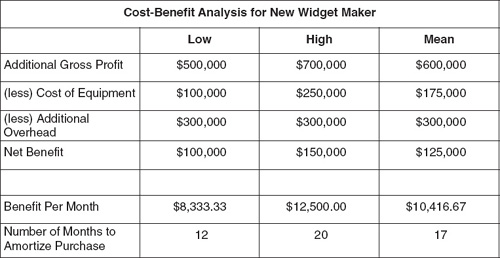
Of course, not all these numbers may be as fixed and known as they appear. In Exercise 7-1, let’s figure out which of these numbers are deterministic and which are probabilistic.
 Exercise 7-1
Deterministic or Probabilistic?
| Number | Deterministic | Probabilistic |
| Make 100,000 new widgets per year with the new equipment | ||
| Sell the additional 100,000 widgets to customers | ||
| Buy a widget maker for a price of $100,000 to $250,000 | ||
| Make a gross profit of $5 to $7 per widget | ||
| Incur overhead costs of $3 per widget sold |
It turns out that only one of our numbers is deterministic, the rest probabilistic. For each of the probabilistic numbers, we have to figure out what values we want to use. And for that, we have to dig a little deeper into the situation.
Expected Monetary Value (EMV)
Our basic risk formula R = P × I is an example of an Expected Monetary Value (EMV) calculation. If there’s a 10% chance of a $10,000 problem (or opportunity), the EMV is $1,000. Of course, you won’t have to pay (or receive) $1,000. You will get one of the two outcomes: no penalty (or benefit), or the full $10,000 (plus or minus).
One benefit of the EMV involves the law of large numbers. A given risk will or will not happen, but of all the risks on your project, some will happen. Let’s imagine we have a project with a base cost of $500,000, and we’ve found 20 minor risks with an average risk score of $1,000 that we choose to accept. If we add $20,000 (20 x $1,000) in contingency allowance to the project, it doesn’t particularly matter to us which of those risks end up consuming the $20,000.
There may be more than one alternative. In that case, the EMV has to add together probabilities and impact for each potential outcome (sometimes referred to as each “state of nature”). Let’s say that for an investment of $8,000, you have a 25% chance of losing $3,000 (you get $5,000 back), a 25% chance of making $2,000 (you get $10,000 back), and a 50% chance of earning $12,000 (you get $20,000 back). Exhibit 7-2 shows how to calculate the EMV.
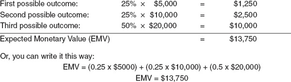
You can compare this EMV to the potential investment to help decide whether it’s worth the risk. Ignoring for the moment the time value of money (let’s assume it’s a short-term investment), the return is $5,750, or 71 percent. Looks good—if you can afford the potential downside of losing $3,000.
In Exercise 7-2, you can try it yourself.
Exercise 7-2
Calculating Expected Monetary Value (EMV)
The Veeblebrox 3000 widget maker produces custom widget designs at a cost of $15 per widget, and produces 1,000 widgets per run. Thirty percent of the time, the widgets are perfect. The rest of the time, there are some defects, shown in the table below. The cost of repairing each defect is $200. What is the EMV cost for 10,000 widgets if you also have $50,000 in fixed costs?
We recommend you use a spreadsheet to solve this problem. If you need help, the formulas are provided separately from the final answer.
| Errors | Likelihood |
| 0 | 30% |
| 1 | 40% |
| 2 | 20% |
| 3 | 10% |
| 5 | 5% |
| 10 | 1% |
Decision Tree Analysis
If you compare the EMVs of different alternatives, choices, or conditions, you create a decision tree. We’ll use the investment we developed in our discussion of expected monetary value, and call that Investment A. The EMV, as you remember, was $13,750, representing a gain of $5,750 on our $8,000 investment.
We have another opportunity, Investment B. This one’s pricier, costing $12,000. It’s also riskier, but it has a very attractive payday. There’s a 60% chance you’ll lose all your investment, a 30% chance you’ll get $20,000, and a 10% chance of making $100,000.
Exhibit 7-3 shows a side-by-side comparison of the two investments using a decision tree.
Here’s how to read it. Start with the question at the left: Which investment (shall we make)? The square to the right of the question represents a decision node. This decision node has two branches, one leading to Investment A and one leading to Investment B. (Forget the “True/False” values for now. They’re added at the very end.)
Investment A has a cost of $8,000. The circle to the right of Investment A is called a chance node. Like a decision node, it generates new branches, but as the name implies, the outcome isn’t up to you. The probabilities and outcomes for each alternative come next. The first outcome of Investment A is that you get back $5,000. This is a net loss of $3,000. Because there’s a 25% chance you’ll get that outcome, the EMV for that branch is -$750.
When we finish calculating all three branches for Investment A, we add up the EMVs for each outcome, and get $5,750. We write that above the decision node—in other words, that’s the EMV for the decision to choose Investment A
xhibit 7-3
Decision Tree
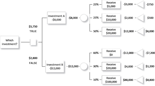
Next, we do the same thing for Investment B, and find that its EMV totals $2,800. We write that below the decision node. And the decision tree is clear: $5,750 beats $2,800. The Investment A decision is labeled TRUE, and the other(s) are labeled FALSE.
 Think About It … (Decision Tree)
What price for Investment B would make it equal in EMV to Investment A?
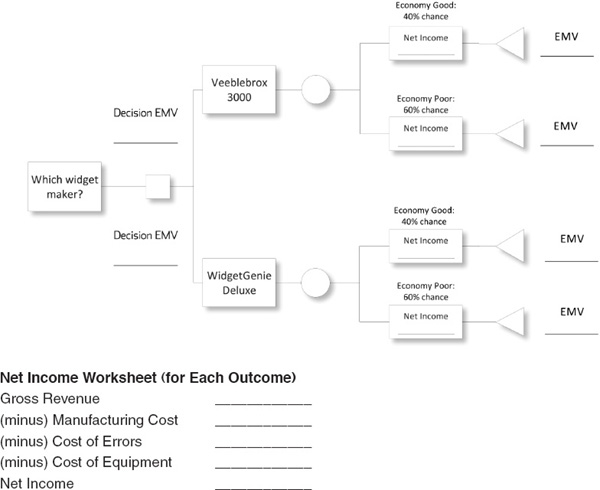
Exercise 7-3
Decision Tree
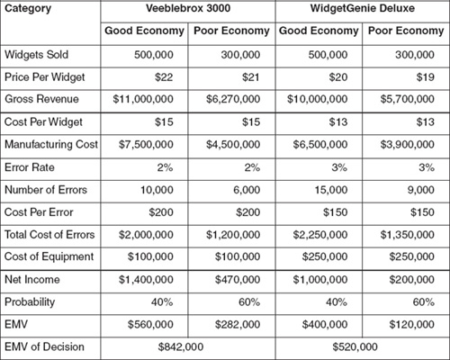
You’re ready to buy a new widget maker, and you’re looking at the Veeblebrox 3000 and the new WidgetGenie Deluxe. The Veeblebrox costs $100,000 and the WidgetGenie costs $75,000. The cost per widget for the Veeblebrox is $15 and for the Widget Genie it’s $12. The Veeblebrox has a net error rate of 2% (repairs cost $200 each) and the WidgetGenie has an error rate of 3% (repairs cost $150 each). If the market is good (40%), you can sell 500,000 widgets a year at $20 per widget, but if it’s poor (60%), sales will only average 250,000 and you can’t get more than $18 per widget.
Which machine is a better buy?
Sensitivity Analysis
If you change an assumption, what happens to the outcome? Let’s continue with the Veeblebrox vs. WidgetGenie example. The Veeblebrox 3000 produces 2% defective widgets, while the WidgetGenie produces 3% defectives. What if the lower defect rate of Veeblebrox widgets allowed you to charge a 10% price premium?
The process of figuring this out is known as sensitivity analysis, the measurement of how a change in a specific assumption or variable affects the bottom line. In this case, the effect is dramatic. Compare the table in Exhibit 7-4 to the answer you developed for Exercise 7-3.
If a 10% price premium changes the decision analysis this drastically, how about some other changes? In Exercise 7-3, use the spreadsheet template you developed in Exercise 7-2 (or copy the one in the answer key), and model the following scenarios. But before you do, make a guess: will this change flip the recommended decision? You may be surprised at which changes make the greatest difference.
Exercise 7-4
Sensitivity Analysis
For each scenario, what are the new EMVs for Veeblebrox and WidgetGenie? Does the decision tree analysis change?
• What if Veeblebrox sold a maintenance package that reduced its error rate to only 1%?
• What if the Veeblebrox was so much faster than the WidgetGenie that you could make and sell 600,000 units in a good economy and 500,000 in a poor economy, as opposed to the WidgetGenie projection of 500,000/300,000?
• What if the cost of fixing Veeblebrox errors dropped from $200 to $100?
• What if WidgetGenie doubles the price on their equipment?

Quantitative tools for risk analysis include cost-benefit analysis, expected monetary value (EMV), decision tree analysis, and sensitivity analysis. They address probabilistic costs, costs with uncertainty. Deterministic costs, in contrast, are fixed and known.
Uncertainty is presented different ways, depending on the purpose for a particular cost estimate. If you want the worst-case scenario, you deliberately pick the most negative assumptions. If you want an average or a median, you develop the estimate accordingly. You should always express a risk-based cost estimate as range, and along with the estimate itself you need to define the scope of the estimate, any assumptions being made, and how long the estimate is likely to remain valid.
Cost-benefit analysis often requires you to price the uncertainties in both costs and benefits; to do so, you must always determine which numbers are deterministic and which are probabilistic.
The expected monetary value (EMV) calculation is essentially the formula for pricing a risk: the probability times the impact summed together for each state of nature. Decision-tree analysis compares EMVs side-by-side to evaluate different decisions or scenarios. Sensitivity analysis measures the effect of a specific change in assumptions or other variables on the bottom line.
These tools are only a selection of what is available. Depending on the specific environment and industry in which you work, you may find additional tools you need.
 Review Questions
1. If a given investment has a 20% of gaining $10,000 and an 80% chance of losing $4,000, what’s the expected monetary value?
(a) + $5,200
(b) - $1,200
(c) - $5,200
(d) + $1,200
1. (b)
2. The term “bottom line” comes from which financial tool?
(a) Cost-benefit analysis
(b) Decision tree analysis
(c) Expected monetary value analysis
(d) Sensitivity analysis
2. (a)
3. A circle in a decision tree diagram indicates:
(a) a decision node from which different outcomes branch.
(b) a chance node from which different outcomes branch.
(c) an end node signifying the final outcome of a given branch.
(d) an EMV calculation of a given risk factor.
4. Using the Veeblebrox/WidgetGenie sensitivity analysis data, what would happen to the buying decision if the cost of repairing defective widgets on the Veeblebrox were the same as for the WidgetGenie?
(a) Veeblebrox 3000 by $250,000
(b) Veeblebrox 3000 by $210,000
(c) WidgetGenie by $270,000
(d) WidgetGenie by $210,000
4. (b)
5. Consider the cost of an insurance policy and the cost of repairing the car in the event of a fender-bender. Which costs are deterministic and which are probabilistic?
(a) Policy cost is deterministic; repair cost is probabilistic.
(b) Policy cost is probabilistic; repair cost is deterministic.
(c) Both costs are deterministic.
(d) Both costs are probabilistic.