
5
Data Retrieval
In Chapter 4 you learned that as the SQL language has evolved, its capabilities have expanded to add more capabilities. In the next two chapters you learn the fundamentals of DML. This chapter introduces the essentials of data retrieval, and Chapter 6 covers data storage and manipulation. Subsequent chapters build on these concepts as you learn about more advanced implementations of these DML components.
Storage and Retrieval
I'm not a particularly organized person by nature. When I am done using an item, my first impulse is to toss it on my dresser or a table. The workbench in my garage hasn't seen the light of day for several months. I tell you this so you can understand my deep appreciation for the orderliness of a relational database. Perhaps this is the element in my life that helps me compensate for the lack of order in other areas. I also love containers of all kinds. The cool thing about having containers is that when you need to put something away, there's always a place for it, but when it comes time to find it, that's often another story.
Retrieving data through queries is really about finding stuff. SQL queries are used to reach into the database and pull out useful information; sometimes you need to get all of the details and sometimes you need only a subset of data based on common characteristics. At times, the value or values you'll want to return are an aggregation of data that tell you something about the data, rather than just returning all of the data in raw form.
I think that the most important statement I can make before diving into the nuts and bolts of SQL is that it's easy. The fundamental mechanics of the language are very straightforward, and this is very much a step-by-step process. Having said that, you will definitely see some complex stuff later on, but it's all based on the same fundamental concepts that are introduced in this chapter.
As you will see later on, queries can be nested within queries and can be saved as programming objects such as functions, stored procedures, and views. Queries can then get their data from these objects. Queries can be joined, nested, and compounded in many different ways. Just remember that it all boils down to the same basic components.
The SELECT Statement
The SELECT statement consists of four clauses or components, as explained in the following table.
| Clause | Explanation |
| SELECT | Followed by a list of columns or an asterisk, indicating that you want to return all columns |
| FROM | Followed by a table or view name, or multiple tables with join expressions |
| WHERE | Followed by filtering criteria |
| ORDER BY | Followed by a list of columns for sorting |
The SELECT statement and FROM clause are required. The others are optional. Think of a table as a grid, like an Excel worksheet, consisting of cells arranged in rows and columns. Often, when you want to view the data in a table, you're only interested in seeing some of the information. To control what data gets returned, you can either display a subset of the columns, a subset of the rows, or a combination of the two. In any case, the result set is a list of rows, each consisting of the same number of columns.
The first few examples in this chapter show you two different views of the same data. I have pasted the contents of the Product table into an Excel workbook. For each query, you will see the first 66 rows and all 10 columns. As I filter the rows and columns, I'll highlight the selected rows and columns. This will provide a different perspective alongside the filtered result set. Keep in mind that Excel presents values a little differently than the results grid. For example, Null values are displayed as empty cells, whereas the results grid displays the text Null, by default (this can be configured to display anything you like). Figure 5-1 shows a sampling of data from the Product table in an Excel worksheet.
Choosing Columns
Specify the columns you want your query to return immediately after the SELECT statement. The following statement returns two columns and all records in the Product table:
SELECT Name, StandardCost, Color FROM Product
Even though there may be dozens of columns of data in this table, you're just returning data values for the ProductID and Name columns. You're still going to get all of the rows that exist in the table. Figure 5-2 shows the Excel worksheet with only the selected columns highlighted.
The result set from the previous query will return only three columns, as shown in Figure 5-3.
If you want to return values for all available columns, you can either specify every column by name or use the asterisk (*) to indicate “all columns.” This query returns all of the columns in the table, as if you had listed every available column in the SELECT statement:
SELECT * FROM Product
Occasionally, I hear the asterisk in this context referred to as a splat. So if you hear an old-timer DBA say “Select Splat From Products,” you'll know what he's talking about.

Figure 5-1
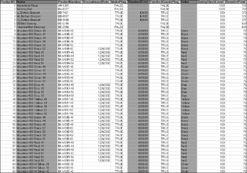
Figure 5-2
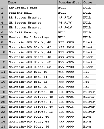
Figure 5-3
There are advantages of using this technique. If the structure of the table were to change, that is, if a column were added or the name changed, this query would continue to return all of the column values based on the table's current design. Likewise, a disadvantage is that if the table's structure were to change, the results might be less predictable. For example, if an application were developed with a form showing employee information, you might expect to see the employee First Name, Last Name, and Phone Number. Later, if a column was added to the table to store salary information, and if this new information was fed to the form, users might inappropriately see sensitive information. This could also destabilize the application, resulting in errors. For this reason, it may be advisable to list all of the columns you want to return. There are a number of reasons to explicitly list the columns in your query, including the following:
- Including columns you don't need produces unnecessary disk I/O and network traffic.
- Sensitive information may be available to unauthorized users.
- In complex, multi-table queries, including all columns produces redundant column values, confusing users and complicating application development.
- Results are more predictable and easier to manage.
Later on, you'll learn about writing queries for multiple tables. In the following Try It Out, you take a look at such a query so you can see how to address columns from more than one table with identical names.
Try It Out
Open SQL Server Query Analyzer or The SQL Server Management Studio and connect to your database server. Select the AdventureWorks2000 database from the selection list on the toolbar. Type the following query into the query editor and execute the query:
SELECT CustomerlD, SalesPersonID
FROM Customer
In the results pane, you should see two columns of values representing customer records — all 19,186 of them. The record count is displayed in the lower status bar, near the right side. Other than possibly the cosmetic differences between SQL Server 2000 Query Analyzer and SQL Server 2005 Management Studio, your results should look something like those shown in Figure 5-4.
Now, expand the query to get sales order information from a related table. Amend the query as in the following example.
Just a quick aside: Although the reason may not be apparent in this example, it's a good idea to get yourself into the habit of formatting your SQL to make it as readable as possible. Note that I have inserted carriage returns before each comma and used tabs and spaces to line up the columns. This is a practice I'll continue to use in the example script, but it is not a requirement.
SELECT CustomerID
     , SalesPersonID
     , PurchaseOrderNumber
FROM Customer
     INNER JOIN SalesOrderHeader
         ON Customer.CustomerID = SalesOrderHeader.CustomerID
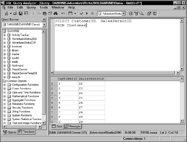
Figure 5-4
Now, when you execute this query, what happens? You get an error that looks like this:
Server: Msg 209, Level 16, State 1, Line 1
Ambiguous column name ‘CustomerID’.
Server: Msg 209, Level 16, State 1, Line 1
Ambiguous column name ‘SalesPersonID’.
The query parser is unhappy because you have referred to two different tables that contain columns with identical names. Both the Customer and SalesOrderHeader tables contain columns named CustomerID and SalesPersonID. This problem is easily remedied by prefixing the column names with the table name. The corrected query would look like this:
SELECT Customer.CustomerlD
     , SalesOrderHeader.SalesPersonID
     , SalesOrderHeader.PurchaseOrderNumber
FROM Customer
   INNER JOIN SalesOrderHeader
      ON Customer.CustomerID = SalesOrderHeader.CustomerID
This works as long as you want to see the ID for the salesperson who actually took the order rather than the one assigned to this customer. As you can see in Figure 5-5, the result set doesn't show you the table name, therefore someone looking at this data may not know to which salesperson you are referring.
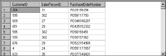
Figure 5-5
SQL Server 2005 Schemas
In SQL Server 2005, table names are prefixed with a schema name, separating the schema name and object name with a period. This practice is common in other database products. For the examples to remain compatible with SQL Server 2000, I am not using schema names. The purpose for schemas is to categorically group objects and make large, complex databases easier to manage. In SQL Server 2000 objects are identified by the four-part name of Server.Database.Owner.Object. SQL Server 2000 does not separate the owner from the schema, but SQL Server 2005 does. This not only creates a namespace to place objects, but also adds a new layer of security to SQL Server by defining a security scope at the schema level. Users in SQL Server 2005 can be assigned a default schema and granted or denied access to specific schemas. Because it's possible to create objects with duplicate names under different schemas, this practice can also lead to a very complex (and possibly confusing) database design. Using schemas is not much different than the practice of assigning different ownership to objects, a capability available in earlier versions of SQL Server, but discouraged.
Here's how it works: The database designer defines schemas, which are really just category names. These schema names can have associated ownership and permissions, which provides the same capabilities available in earlier SQL Server versions. The implementation is very simple. In the AdventureWorks2000 database, you reference the Product table in a query like this:
SELECT * FROM Product
If you were using the AdventureWorks database that installs with SQL Server 2005, because the Product table is in the Production schema, you must use this syntax:
SELECT * FROM Production.Product
In SQL Server 2000 and earlier versions, objects are typically owned by a user called DBO, and if you don't prefix an object reference with a username, the DBO user is just assumed. The same is true with schemas in SQL Server 2005. Objects can belong to the DBO schema, and if you don't use a schema name in an object reference, the DBO schema is assumed. However, this is only true if your default schema has not been changed to something other than DBO. If an object is part of any other schema, the schema name must be used in the expression. Here is an example to illustrate this new feature.
User Fred connects to the AdventureWorks database on a SQL Server 2005 instance called Bedrock1. Fred's default schema has not been changed and so it is set to DBO. Fred then executes the following query:
SELECT * FROM Product
The Query Processor attempts to resolve the Product table name to Bedrock1.AdventureWorks.dbo. Product, but the query fails because the Product table exists in the Production schema and not the DBO schema. Now I change Fred's default schema like this:
ALTER USER Fred WITH DEFAULT_SCHEMA = Production
When Fred executes the product query again, the Query Processor resolves the product table to Bedrock1.AdventureWorks.Production.Product and the query succeeds.
Now take a look at an opposite example. User Barney connects to the same instance that user Fred did, but he wants to retrieve the contents of the SalesOrder table that exists in the DBO schema. Barney's default schema has also been set to Production. Barney runs the following query:
SELECT * FROM SalesOrder
The Query Processor first attempts to resolve the SalesOrder table to Barney's default schema; Bedrockl.AdventureWorks.Production.SalesOrder, but the resolution fails. However, because the Query Processor started in a schema other than DBO, it then falls back to the DBO schema and attempts to resolve the table to Bedrockl.AdventureWorks.dbo.SalesOrder. This resolution succeeds and the contents of the table are returned.
Column Aliasing
You may want to change column names in a query for a variety of reasons. These may include changing a column name to make it easier to understand or to provide a more descriptive name. Changing a column name can also provide backward compatibility for application objects if column names were renamed after design.
In a previous example you saw that the Query Processor needs to know what table to retrieve a column from if the column exists in more than one referenced table. The same can also be true for the person reading the results. They might need to know exactly what table the values were extracted from. The following example clarifies the source of an ambiguous column by using an alias:
SELECT Customer.CustomerID
     , SalesOrderHeader.SalesPersonID AS OrderSalesPersonID
     , PurchaseOrderNumber
FROM Customer
   INNER JOIN SalesOrderHeader
      ON Customer.CustomerID = SalesOrderHeader.CustomerID
In the result set shown in Figure 5-6, you can see that the second column now shows up as OrderSalesPersonID.
Months later, this could save someone a lot of grief and aggravation. Imagine getting a call from the accounting department when they discover that they have been paying commission to the wrong salespeople.
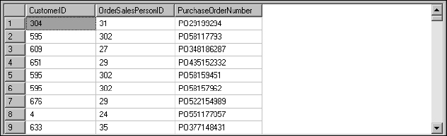
Figure 5-6
You can alias a column in three different ways. The technique used in the preceding example is probably the most descriptive. A popular technique leaves out the AS keyword so the actual column name simply precedes the alias. The following table shows each of these techniques. The last one isn't common, and I don't recommend that you use it. However, this may come in handy if you come across a script containing this syntax.
| Syntax | Description |
| Column AS Alias | Most readable technique, however, not popular with SQL purists. |
| Column Alias | Most common technique. Most auto-generated code is written in this form. |
| Alias = Column | This technique is not common in Transact-SQL. |
Here are examples of these three techniques:
SELECT FirstName + ‘ ’ + LastName AS FullName
FROM Contact

SELECT FirstName + ‘ ’ + LastName FullName
FROM Contact

SELECT FullName = FirstName + ‘ ’ + LastName
FROM Contact
Calculated and Derived Columns
One of the most common types of column aliases is when a new column is created from an expression or calculation. In the following example using the Employee table, the employees' first name and last name are combined (or concatenated) together. Character concatenation can be performed using the plus sign, like so:
SELECT FirstName + ‘ ’ + LastName AS EmployeeName
FROM Employee
This produces a single column called EmployeeName, which contains the employees' first name, a space, and then their last name, as shown in Figure 5-7.
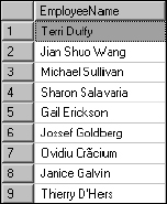
Figure 5-7
Character data isn't the only thing you can manipulate to produce new column values. A few examples using various functions and column data types follow. This first simple example uses the UnitPrice and OrderQty columns from the SalesOrderDetail to calculate the purchase amount for a line item by multiplying these two values. The resulting alias column is called PurchasePrice:
SELECT SalesOrderID
     , LineNumber
     , ProductID
     , UnitPrice * OrderQty As PurchasePrice
FROM SalesOrderDetail
In the result set shown in Figure 5-8, the PurchasePrice column shows the calculated figure.
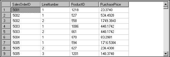
Figure 5-8
In the following scenario, you need to calculate each employee's age based on their birth date and the current date. Using the DateDiff function, you ask SQL Server to calculate the number of days between the two dates and then divide by 365 to get the approximate result in years. The query would look like this:
SELECT FirstName
     , LastName
     , BirthDate
     , DateDiff(Day, BirthDate, GetDate())/3 65 As Age
FROM Employee
The result set should look like that shown in Figure 5-9.
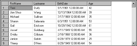
Figure 5-9
In this example, the Product table, the SubCategoryID, is related to a column in the ProductSubCategory table. Without using a join between these tables, I would like to see the subcategory name in the output from my query. Because I know that SubCategoryID 1 represents mountain bikes, I can add this description using an alias column. In the WHERE clause, I filter product rows based on the subcategory and then add an alias column called SubCategoryName:
SELECT Name, ListPrice, ‘Mountain Bike’ AS SubCategoryName
FROM Product WHERE ProductSubCategoryID = 1
Figure 5-10 shows the results from this query. Note the SubCategoryName column.

Figure 5-10
I'll come back to this example and expand on it in Chapter 8 when you learn about Union queries.
Filtering Rows
It's safe to say that most of the time you won't want to return every record, especially in your largest tables. Many production databases in business are used to collect and store records for many years of business activity. For small to medium-sized businesses, this is a common practice. In larger-scale systems, data is usually archived yearly or monthly and useful, historical information may be moved into a data warehouse for reporting. Regardless, it often doesn't make sense to return all rows in a table. Two basic techniques exist for returning some of the rows from a query: The WHERE clause is used to qualify each row based on filter criteria, and the TOP clause is used to truncate the list after a certain number of rows are returned.
The WHERE Clause
Filtering is largely the job of the WHERE clause, which is followed by some sort of filtering expression. The syntax of this statement is very natural and should be easy to translate to or from a verbal statement. I'll continue to use the Excel worksheet example that I began using earlier in this chapter. In this example, all columns for product rows where the color is black are returned:
SELECT * FROM Product
WHERE Color = ‘Black’
I'm essentially asking SQL Server to filter the rows for the table only vertically, returning slices that meet only the specified color criteria, as reflected in Figure 5-11.
The result set shows only the matching rows (as much as you can see in the results grid), as shown in Figure 5-12.
Recall that I used this workbook to demonstrate selecting specific columns to be returned from the query. So far, I've selected specific columns and specific rows. Now, I'll combine the two to return a subset of both columns and rows using the following SELECT expressions:
SELECT Name, StandardCost, Color
FROM Product
WHERE Color = ‘Black’
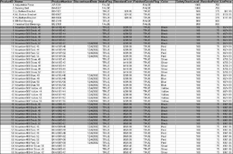
Figure 5-11

Figure 5-12
Before showing you the results, Figure 5-13 gives you another look at that workbook data with highlighted columns and rows.
The result set contains only the values in the intersection of the columns and rows. As you can see in Figure 5-14, only the Name, StandardCost, and Color columns are included, and the only rows are those where the Color value is Black.

Figure 5-13
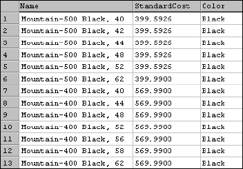
Figure 5-14
For example, consider the following verbal request: “I would like to see a list of products, including the product name and price that have a price less than $5.00.” The SQL version of this request would look like this:
SELECT Name, ListPrice
FROM Product
WHERE ListPrice < 5.00
Only five products meet these criteria, as shown in Figure 5-15.
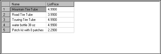
Figure 5-15
Easy, right? Filtering statements should be very natural and easy to read. You just need to get used to the flow.
Comparison Operators
Qualifying values to match a set of criteria is a relatively straightforward proposition, especially when working with numeric and date/time types. Testing a numeric value to see if it is greater than 10 makes sense and there is little room for confusion. However, testing to see if the value Fred is greater than the value Bob may not make much sense.
Comparing and qualifying values generally boils down to this: A value is either equal to, less than, or greater than another value. When matching character values, you can be a little more creative, looking for partial strings of characters to match a value that is “like” another value. Starting with the simplest comparisons, value-matching operators are described in the following table.
Logical Comparisons
Using logical comparisons is how we make sense of things and it's how we simplify matters. It's how we dispel the gray area between yes and no or true and false.
It would be convenient if all decisions were based on only one question, but this is rarely the case. Most important decisions are the product of many individual choices. It would also be convenient if each unique combination of decisions led to a unique outcome, but this isn't true either. The fact is that, often, multiple combinations of individual decisions can lead to the same conclusion. This may seem to be very complicated. Fortunately for us, in the 1830s mathematician George Bool boiled all of this down to a few very simple methods for combining outcomes called logical gates. There are only three of them: And, Or, and Not.
It's important to realize that every SQL comparison and logical expression yields only one type of result: True or False. When combining two expressions, there are only three possible outcomes: they are both True, they are both False, or one is True and the other False. With the groundwork laid, let's apply Bool's rules of logic to the SQL WHERE clause and combine multiple expressions.
The AND Operator
The AND operator simply states that for the entire expression to yield a True result, all individual statements must be true. For example, suppose you're looking for product records where the SubCategoryID is 1 (mountain bikes) and the price is less than $1,000. You're not interested in road bikes under $1,000, nor mountain bikes costing $1,000 or more. Both criteria must be met.
Assuming that there are records matching either criterion, the AND operator will always reduce the rows in the result set. For example, the Product table contains 142 mountain bikes and 478 rows with a list price under $1,000. However, only 54 rows match both of these filters. Figure 5-16 shows 9 of them.
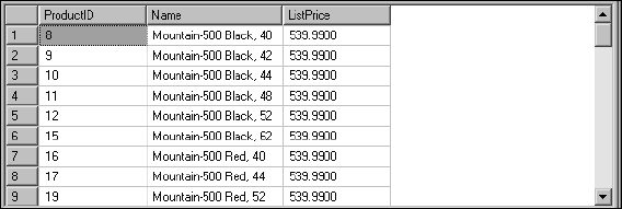
Figure 5-16
The OR Operator
When statements are combined using the OR operator, rows are returned if they match any of the criteria. Using the previous statement, changing the AND to an OR produces a different result:
SELECT ProductID, Name, ListPrice
FROM Product
WHERE ProductSubCategoryID = 1 OR ListPrice < 1000
Rather than seeing only mountain bikes under $1,000, you see all mountain bikes, regardless of their price, and all products having a price under $1,000. This query returns 521 rows (9 of which are shown in Figure 5-17). Note that even though there would be less expensive mountain bikes in either of the combined results, SQL Server is smart enough to remove the duplicate rows.
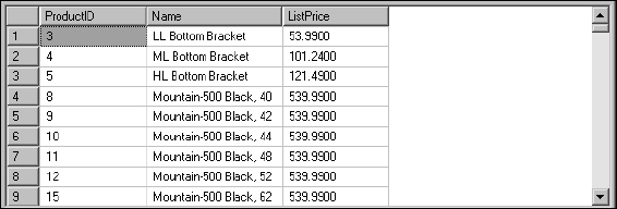
Figure 5-17
The NOT Operator
The NOT operator doesn't stand alone. It's simply a modifier that can precede any logical expression. The job of this operator is to reverse the result. So, if an expression yields True, you get a False. If it's False, you see True. Sometimes it's easier to test for the opposite of what you are looking for. However, the NOT operator is often less efficient because SQL Server actually processes the base expression first (perhaps returning all qualifying rows), and then fetches the rows that were not included in the original result. Depending on the complexity of the statement and the number of rows in the table, using NOT may still be more efficient than having to build an expression that selects everything but the records you want to ignore.
If you wanted to return all product records except for road bikes, you could use this expression:
SELECT ProductID, Name, ListPrice
FROM Product
WHERE NOT ProductSubCategoryID = 2
In the result set, shown in Figure 5-18, all rows are returned except for those having a SubCategoryID value of 2.
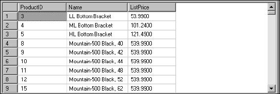
Figure 5-18
The Mighty Null
In the earlier days of databases, designers often found it difficult to consistently express the concept of “no value.” For example, if a product invoice line is stored but you don't have the price of the product at the time, do you store a zero? How would you differentiate this row from another where you intended not to charge for the product?
Character data can be particularly strange at times. Within program code, string variables initialize to an empty string. In older file-based databases, what would now be considered to be a field would consist of a designated number of characters in a specific position within the file. If a field wasn't assigned a value, the file stored spaces in place of the data. Programs returned all of the characters including the spaces, which had to be trimmed off. If there wasn't anything left after removing the spaces, the program code concluded that there was no value in the field. So, what if you had intended to store spaces? How would you differentiate between a space and no value at all? Numeric types initialize to zero. The Bit or Boolean data type in some programming languages initializes to zero or False. If you store this value, does this mean that the value is intentionally set to False, or is this just its default state? What about dates that haven't been set to a value? As you can see, there is plenty of room for confusion regarding this topic. For this and other reasons, the ANSI SQL standard for representing the concept of “no value” is to use a special value called Null. Internally, Null is actually a real character (on the ANSI character chart, it's character zero—not to be confused with the number zero). It means “nothing,” that this field doesn't have a value. Every significant data type supports the use of the Null value.
The Null value has an interesting behavior—it never equals anything, not even itself. To make it stand out, a special operator distinguishes Null from all other values. To test for Null, use the IS operator. So, Null does not equal Null… Null IS Null.
Some of the product records don't have a standard cost. To intentionally state that the product does not have a cost (or, perhaps, that the cost isn't known), this column is set to Null. Now you'd like to return a list of products with no recorded cost, so you use the following query:
SELECT ProductID, Name, StandardCost
FROM Product
WHERE StandardCost IS NULL
The results contain no StandardCost values, as shown in Figure 5-19.

Figure 5-19
To reverse the logic and return a list of the products with a known cost, you simply add the NOT operator, like so:
SELECT ProductID, Name, StandardCost
FROM Product
WHERE StandardCost IS NOT NULL
The result should contain all of the rows from this table that were not listed in the previous result, some of which are shown in Figure 5-20.
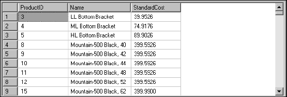
Figure 5-20
Extended Filtering Techniques
As you've seen, expressions using simple comparison operators can be combined to narrow down results and explicitly return the records you are looking for. Sometimes, even simple filtering expressions can get a little complicated. To simplify common expressions, operators were added to the SQL language. If nothing more, it makes expressions more natural and easier to read. One common example is a query for records in a date range. If you needed to return all employee records for employees born between 1962 and 1985, you would need to specify that the birth date should be greater than or equal to the first day of the first year in the range, January 1, 1962, and that the same column should also be less than or equal to the last day of the last year, December 31, 1985. This query would look like this:
SELECT FirstName, LastName, BirthDate
FROM Employee
WHERE BirthDate >= ‘1-1-62’ AND BirthDate <= ‘12-31-85’
The results contain only Employee records where the birth date falls within the specified range, as shown in Figure 5-21.
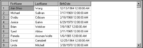
Figure 5-21
The BETWEEN Operator
Rather than managing the date range, the BETWEEN statement simplifies the range expression, helping state your intentions more explicitly:
SELECT FirstName, LastName, BirthDate
FROM Employee
WHERE BirthDate BETWEEN ‘1-1-62’ AND ‘12-31-85’
Granted, the first statement wasn't really that complicated, but if you combine this expression with others in the same query, every attempt to simplify a query helps. Keep in mind that the definition of BETWEEN is actually between and including both extremes of the value range.
When the query is executed, SQL Server's query parser analyzes the expression and reformats the query in more explicit, standardized form. Essentially, if you wrote and executed the second query using the BETWEEN statement, the query that actually runs against the query engine would be similar to the first.
The IN() Function
This function is designed to match a field to any number of values in a list. This is another shortcut to save effort and keep your queries shorter and easier to read. For example, suppose that you're interested in a list of customers in your western sales region. You have no region designation in the database but you know this consists of the following states: Washington, Oregon, California, Idaho, and Nevada. The state/province codes are stored in a table called StateProvince. To keep things simple, I'm going to show you two examples. The first just returns the state names from the StateProvince table. The second example joins several tables together, solving the business problem before you. This expression is necessary due to the complexity of the AdventureWorks2000 database. For the first example, type the following into the query editor:
SELECT Name FROM StateProvince
WHERE StateProvinceCode IN (‘WA’, ‘OR’, ‘CA’, ‘ID’, ‘NV’)
The more realistic example is a little more complex and involves some elements that haven't been covered yet. Don't be concerned with the mechanics of the joins for now. Nevertheless, the following query joins four tables together to return a list of stores and the states in which they reside:
SELECT Store.Name, StateProvince.Name
FROM Store
  INNER JOIN CustomerAddress ON Store.CustomerID = CustomerAddress.CustomerID
  INNER JOIN Address ON CustomerAddress.AddressID = Address.AddressID
  INNER JOIN StateProvince ON Address.StateProvinceID =
StateProvince.StateProvinceID
WHERE StateProvince.StateProvinceCode IN (‘WA’, ‘OR’, ‘CA’, ‘ID’, ‘NV’)
Take a look at these results shown in Figure 5-22. Note that although you are filtering on the StateProvinceCode column, which contains the two-letter state abbreviation, you're returning the StateProvinceName column containing the full name for readability.
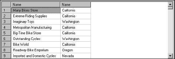
Figure 5-22
Note that the column names are the same. This is possible because they came from two different tables. If this were a production query, the next step I'd recommend would be to alias these columns with unique names. Otherwise, it's a little confusing to see two columns called “Name.”
Operator Precedence
It's important to consider the order in which multiple operations are carried out. If not, you may not get the results you'd expect. The precedence (order of operations) is determined by a few different factors. The first and most important is whether the precedence is explicitly stated. This is covered shortly. Operations involving different data types may be processed in a different order. Lastly, the operators are considered: NOT is processed first, then AND, then OR operations. Before you look up this topic in Books Online and attempt to memorize the operator precedence for every data type, please read on.
Here's an example. A user says that she would like a list consisting of mountain bikes and road bikes priced over $500 and under $1,000. You know that the product subcategories for mountain bikes and road bikes are 1 and 2, respectively. This query follows the logic of the stated requirement:
SELECT Name
       , ProductNumber
       , ListPrice
       , ProductSubCategoryID
FROM Product
WHERE
       ProductSubCategoryID = 1 OR ProductSubCategoryID = 2
  AND  ListPrice > 500 AND ListPrice < 1000
If you run this query, you see that it returns 199 records that appear to meet the requirements (see Figure 5-23).

Figure 5-23
However, upon closer examination, you can see that you have $4,000 mountain bikes on the list. Why is that? Go back and take a look at the query. When the query parser has to contend with more than one logical operator, it has to decide how to process them. It will always process an AND expression before an OR expression. The mechanics of query processing are really up to the query optimizer, but the results for a given statement will always be the same. Later on you'll learn how to find out what the query optimizer does when it breaks down and processes a query. Most likely, in this case, it took the first AND expression,
ProductSubCategoryID = 2 AND ListPrice
processed and buffered the results, and then the next AND expression,
AND ListPrice < 1000
and used this to filter the first set of results. So far, so good, but it's the next step that gets you into trouble. Because the query parser processes an OR expression after all of the AND logic, it went back to the beginning of the WHERE clause and processed this statement:
ProductSubCategoryID = 1
Because this statement preceded the OR operator, it found all of the mountain bike records in the table and appended these to the first set of results. So the query processor did what you told it to do but not necessarily what you wanted it to do.
SELECT Name
       , ProductNumber
       , ListPrice
       , ProductSubCategoryID
FROM Product
WHERE
       ListPrice > 500 AND ListPrice < 1000
  AND  ProductSubCategoryID = 1 OR ProductSubCategoryID = 2
This query returns 238 rows, including expensive road bikes:
SELECT Name
       , ProductNumber
       , ListPrice
       , ProductSubCategoryID
FROM Product
WHERE
       ProductSubCategoryID = 1
  AND  ListPrice > 500 AND ListPrice < 1000
   OR  ProductSubCategoryID = 2
Frankly, rearranging these statements will not give you the results you're looking for. Unless you find a way to tell the query-processing engine the order in which you want it to process these operations, you're not going to get a list of affordable bikes.
Using Parentheses
Filter expressions are often combined to return a very specific range and combination of records. When combining the individual expressions, it's often necessary (or at least a good idea) to use parentheses to separate expressions and to specify the operation precedence and order. Making a point to use parentheses when multiple operations are processed makes it unnecessary to be concerned with the complexities of normal operator precedence.
For example, I would like a list consisting of mountain bikes priced over $1,000 and road bikes priced over $500. I know that the product subcategories for mountain bikes and road bikes are 1 and 2, respectively. My query looks like this:
SELECT Name
       , ProductNumber
       , ListPrice
       , ProductSubCategoryID
FROM Product
WHERE
     (ProductSubCategoryID = 1 AND ListPrice > 1000)
  OR
     (ProductSubCategoryID = 2 AND ListPrice > 500)
The parentheses in this example serve only to clarify the order of operations. Because the AND operator is processed before the OR operator, the parentheses are not actually necessary in this expression. Using the same comparisons with a different combination of operators would yield different results, unless the appropriate application of parentheses was applied. The following queries exemplify this point. This first example (with or without parentheses) returns 272 rows. The following query is the same, only with the parentheses removed:
SELECT   Name
       , ProductNumber
       , ListPrice
       , ProductSubCategoryID
FROM Product
WHERE
     ProductSubCategoryID = 1 OR ListPrice > 1000
  AND
     ProductSubCategoryID = 2 OR ListPrice > 500
This query returns 563 rows (a sampling of which is shown in Figure 5-24).
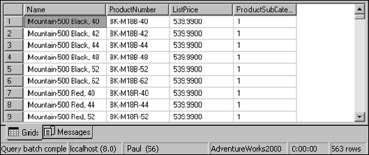
Figure 5-24
With parentheses grouping the two OR operators and separating the AND operators, the same query returns 420 rows:
SELECT   Name
      , ProductNumber
      , ListPrice
      , ProductSubCategoryID
FROM Product
WHERE
     (ProductSubCategoryID = 1 OR ListPrice > 1000)
  AND
     (ProductSubCategoryID = 2 OR ListPrice > 500)
The results are shown in Figure 5-25.

Figure 5-25
The bottom line is, whether or not parentheses are required, use them to state your intentions and to make your queries easier to read. When multiple operations are combined, it becomes increasingly important to group and separate operations using parentheses. Just as in mathematical expressions, parentheses can be nested any number of levels deep.
Sorting Results
Typically, you will want records to be returned in some sensible order. Rows can be sorted in order of practically any combination of columns. For example, you may want to see employee records listed in order of last name and then by first name. This means that for employees who have the same last name, records would be sorted by first name within that group. When writing and testing queries, you may see that some tables return rows in a specific order even if you don't make it a point to sort them. This may be due to existing indexes on the table, or it may be that records were entered in that order. Regardless, as a rule, if you want rows to be returned in a specific order, you should use the ORDER BY clause to enforce your sorting requirements and guarantee that records are sorted correctly if things change in the table.
The ORDER BY clause is always stated after the WHERE clause (if used) and can contain one or more columns in a comma-delimited list. If not stated otherwise, values will be sorted in ascending order. You can optionally specify ascending order using the ASC keyword. This means that the following two statements effectively do the same thing:
Or
SELECT FirstName, LastName FROM Employee ORDER BYy LastName ASC
As you see, records are sorted by the LastName column. In the result set shown in Figure 5-26, I've scrolled down the list to view Brown and Campbell.

Figure 5-26
Note that the first name values for Kevin and Jo Brown and for John and David Campbell are out of order. As far as we're concerned, this order is completely arbitrary. You can correct this by adding the FirstName column to the ORDER BY list, like so:
SELECT FirstName, LastName FROM Employee ORDER BY LastName, FirstName
Now the results show employees sorted in order of LastName and then subsorted by FirstName. Jo, Kevin, David, and John now appear alphabetically, as shown in Figure 5-27.

Figure 5-27
One more example shows how rows can be sorted in descending order. Suppose that you want to have your employees listed in order of age, youngest first. This is a simple task. Using the ORDER BY clause, indicate that the BirthDate column should be sorted in descending order:
SELECT FirstName, LastName, BirthDate
FROM Employee ORDER BY BirthDate DESC
The result shown in Figure 5-28 starts with employees born in 1979.

Figure 5-28
Just a side note to clarify what you see here: The DateTime data type stores both the date and time. In this case, the time wasn't actually entered for these birth dates but defaults to 12:00:00 AM, or midnight.
Top Values
So far, you've seen that if you want to return a subset of the rows in a table, it's necessary to filter the results based on some sort of criteria. In some cases, you will want to simply return a specific number of records regardless of the number of qualifying rows. You have two options for returning top values: including a fixed number of rows or a percentage of total rows.
This example also involves the ages of employees in the AdventureWorks2000 database. Like the previous example, the following query returns a list of all employees sorted by their birth date, or age, oldest to youngest (in this case, sorting by birth date in ascending order):
SELECT FirstName, LastName, BirthDate
FROM Employee
ORDER BY BirthDate
The first few rows in the result set look like those shown in Figure 5-29.
Now, add the TOP statement to indicate that you really only want to see the first five rows in the result set:
SELECT TOP 5 FirstName, LastName, BirthDate
FROM Employee
Order By BirthDate
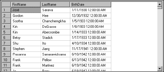
Figure 5-29
As you see in the following result set, shown in Figure 5-30, only five rows are returned.
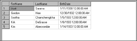
Figure 5-30
SQL Server doesn't try to make much sense out of this data. It doesn't even consider the sorted values when chopping off the list. It simply truncates the results after the fifth row has been returned, regardless of any values. This point is more apparent in the following example. The next query returns products in order of their price. I've made it a point to sort the product list in descending order of list price. This puts the most expensive products at the top of the result list:
SELECT Name, ListPrice
FROM Product
ORDER BY ListPrice Desc
For the bicycles, a unique product record represents a different color and frame size, so there are actually several rows for the same model. The most expensive bike, the road bike model 150, costs $3,578.27. Given all of the color and frame size combinations, there are 28 products at this price. If you were to ask for the top five list of bikes (and you're sorting only on price), the list is arbitrarily truncated after five records:
SELECT TOP 5 Name, ListPrice
FROM Product
ORDER BY ListPrice Desc
Keep this in mind when asking for a “top” list.
WITH TIES
There is an easy way to solve the dilemma caused by tied values in the last position of your top list arbitrarily capping the results. First of all, you need to go back and clarify the business rule. Often, this means going back to your users or project sponsor to seek a restatement of requirements. That conversation might go something like this:
“You said that you wanted a report showing the top 25 most expensive products. What if the price of the 25th product were the same as another product—or more—down the list? Do you want to include other products that are tied for the same price as the item in the 25th position?”
If the answer is “Yes,” the solution is quite simple. The WITH TIES statement simply continues to populate the list as long as subsequent rows' sorted values are the same as the last item in the Top list. For example, the following requests a list of the top 25 most expensive products using the same statement as before, except using Top 25 WITH TIES:
SELECT TOP 25 WITH TIES Name, ListPrice
FROM Product
ORDER BY ListPrice DESC
Figure 5-31 shows the complete results for this query.
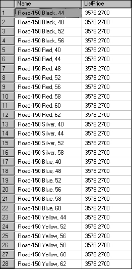
Figure 5-31
As you can see, 28 rows are returned because rows 26, 27, and 28 have the same ListPrice value as row 25.
Try It Out
To bring this topic full circle, go back to the original example and do the same thing with employee birth dates. Using the same query as before, add the Top 11 statement. Execute this query:
SELECT TOP 11 FirstName, LastName, BirthDate
FROM Employee
ORDER BY BirthDate
Now add the WITH TIES statement:
SELECT TOP 11 WITH TIES FirstName, LastName, BirthDate
FROM Employee
ORDER BY BirthDate
How It Works
SQL Server does exactly what you asked it to do: it returns 11 rows. You should get 11 employee records returned with Frank Martinez in the last position when you write the query without WITH TIES. His birth date is 6/19/1942. However, Frank shares his birthday with Jo Berry, who happens to be in the next position. When you use the WITH TIES modifier, Jo shows up in position 12 on your top 11 list. SQL Server will continue to output rows until the sorted value changes.
Note that records 11 and 12 in Figure 5-32 have the same value in the BirthDate column.
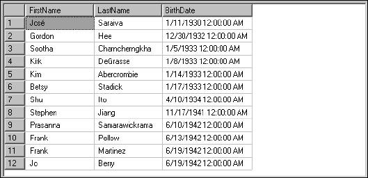
Figure 5-32
Percent
Rather than specifying a number of records to be returned with the TOP statement, you can also specify a percentage of the entire result set. SQL Server will do the math for you and then round to the nearest whole number. It essentially performs this calculation and then issues a Top X clause in place of the Top X Percent. Do this using the birth date example. If you were to select all employee records, without using the TOP statement, 292 rows would be returned. If you ask for the top 10 percent, a subset of rows is returned. Try it out:
As you can see in Figure 5-33, 30 rows are returned. This is because SQL Server rounds up to the nearest whole record.
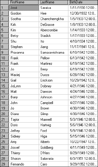
Figure 5-33
The same rules apply as if you had just used the Top X version of this statement. You can use WITH TIES and sort the result in either ascending or descending order.
Summary
Although you haven't seen a lot of complexity in this introduction to the SELECT statement and its fundamental nuances, it's a very powerful tool. As you continue to build more complex statements, the SELECT statement will be center stage. This chapter started by explaining selecting all rows using the asterisk (*) to return values for all available columns in a table and then moved on to specify selected columns. It is more efficient to return only the columns needed. This is especially the case when standard queries will be called routinely by software code, a report, or an application component. You learned how columns can be aliased to either rename a column or return a new column from a literal value, calculation, or expression based on multiple column values.
Filtering rows is the function of the WHERE clause, using logical comparisons. Values may be equal to, less than, greater than, or the opposite of any of the above by using the NOT operator. Character data types can also be compared using the LIKE operator to perform partial matching, wildcard, and pattern matching. Using Null is the accepted method to indicate that a column value has not been set—and testing for Null gives you an exact method to test for this condition. When combining comparison operators, it's often necessary to indicate the order of operations using parentheses. Not only does this ensure that operations are performed in the appropriate order, but it also makes queries much easier to read and maintain.
Rows can be sorted on any number of columns and can be placed in ascending or descending order. Finally, this chapter discussed the use of the TOP keyword, used to truncate a result set either by a specific number of rows or by a percentage of the entire result set.
Exercises
Exercise 1
Using Query Analyzer or SQL Server Management Studio, write a query to return Employee records from the AdventureWorks2000 database. Include only the FirstName, LastName, and EmailAddress columns in the result set. Execute this query and view the results.
Exercise 2
Return Employee records from the AdventureWorks2000 database. Combine the FirstName and LastName columns separated by a space, to return an aliased column called FullName. Return only the FullName and Title columns. Sort the results by the LastName and then FirstName columns in ascending order.
Exercise 3
Return Product records that have a DiscontinuedDate value greater than or equal to December 4, 2002. Include the Name and ListPrice columns.
Exercise 4
Return a list of Department records including all columns.
Include only departments that have a Name value ending with the word Control. These records must also have a Name column value starting with the word Production. In addition to these records, include records that have a GroupName value ending in the word Assurance.
Sort these records by the Name column in reverse alphabetical order.