7

Aggregation and Grouping

Information is meaningful; data is just values stored in a table. Often, the information part of the equation comes from analyzing groups of records and comparing how one range of records relates to another. For example, rather than viewing individual sales records, you may be interested in comparing the total sales of a product in one region to another or, perhaps, the average price of mountain bike sales with the average price of road bike sales.

The term aggregation refers to something that is a part of something else. In this context, an aggregate function returns a single value for a group of records. You can use aggregate functions in two different ways. You can “roll up” or summarize all of the rows returned by a query (either all records or use filtering techniques as discussed in Chapter 5). Aggregation can also be applied at a group level, showing summarized values for the rows having the same values in the columns you designate for grouping.

Using Aggregate Functions

The simplest technique is aggregating all rows in a query. Aggregate functions include the means to summarize a range of values in a variety of ways. You may simply want to count the rows that match a criterion or get the sum of a range of numeric values. The following table contains all of the system-supplied aggregate functions supported by Transact-SQL used to summarize column values.

The COUNT() Function

The COUNT() function simply counts rows or non-null values in a column's value range. Because the data type of the column isn't considered, it will work with columns of practically any type of data. Consider the following two examples. If you execute this query against the Product table, the total number of rows is returned:

SELECT COUNT(*) FROM Product

As you can see, the Product table contains 999 rows. Now, count only the values in the ListPrice column using the following expression:

SELECT COUNT(ListPrice) FROM Product

Because 200 records don't have a ListPrice value (these rows contain the value NULL for this column), only 799 rows get counted. Now add the word DISTINCT before the column reference and execute the query again:

SELECT COUNT(DISTINCT ListPrice) FROM Product

Because so many of the products have the same prices, only 104 records are counted. The DISTINCT modifier can be used with any of the aggregate functions except when using the CUBE or ROLLUP statements, which are discussed later in this chapter.

The SUM() Function

The SUM() function simply returns the sum of a range of numeric column values. Like the others, this function only considers non-null values. A simple example returns the subtotal for a product order. This query adds up the UnitPrice for each detail line in the order whose SalesOrderID is 5005:

SELECT SUM(UnitPrice)
FROM SalesOrderDetail
WHERE SalesOrderID = 5005

The result is a single row with a single column just like the previous examples, as shown in Figure 7-1.

Figure 7-1

I have two issues with this result. The first is that the column doesn't have a name. When applying aggregate functions, the resulting column won't be named unless you specifically define an alias for the column name. If you use visual query design tools, such as Access or the Transact-SQL Designer (in Visual Studio or to create a view in Enterprise Manager), these tools will devise column aliases such as SumOfUnitPrice or Expr1. The first order of business is to assign an alias so this column has a sensible name. The other problem with this simple example is that it assumes that the customer purchased one of each product. The fact is that there are three detail rows for this order with respective quantities 1, 3, and 4. To accurately total the order, you'll have to do a little math. This query resolves both of these issues, calculating extended price and defining an alias for the column:

SELECT SUM(UnitPrice * OrderQty) As OrderTotalPrice
FROM SalesOrderDetail
WHERE SalesOrderID = 5005

The result shown in Figure 7-2 contains the correct amount (the total of all three order detail rows, considering the quantity for the product purchased), and the column has a name.

Figure 7-2

The AVG() Function

The AVG() function returns the calculated average for a range of numeric values. Internally, the query processor calculates the sum of all the values and then divides by the number of rows in the range (containing non-null values.) Optionally, the AVG() function can make a distinct selection of values and then perform the same calculation on this abbreviated set of values. Using a distinct selection can greatly affect the results and is not as common.

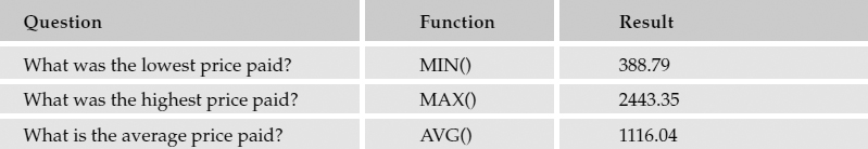
I'd like to use the product sales data in the AdventureWorks2000 database to demonstrate the practical application of these functions. In this scenario, the director of marketing has asked for an analysis of road bike sales in 2003. This information exists in three related tables. Pay no attention to the join statements for the time being; they are covered in Chapter 8. The following query uses the SalesOrderHeader table to filter the sales order, the Product table to filter by ProductSubCategoryID (2 is road bikes), and the UnitPrice is retrieved from the SalesOrderDetail table. For simplicity, I'm not considering the quantity of bikes purchased.

I'll start with the lowest price paid for a bike. Using the MIN() function should return only one value:

SELECT   MIN(UnitPrice)
FROM     SalesOrderHeader
         INNER JOIN SalesOrderDetail ON
         SalesOrderHeader.SalesOrderID = SalesOrderDetail.SalesOrderID
         INNER JOIN Product ON SalesOrderDetail.ProductID = Product.ProductID
WHERE    Product.ProductSubCategoryID = 2
         AND SalesOrderHeader.OrderDate BETWEEN ‘1-1-03’ And ‘12-31-03’

You can see that the lowest UnitPrice value in this range is $388.79. Just modify the query, substituting the following functions in place of the MIN() function in the example. The following table shows the results.

Understanding Statistical Functions

Statistics wasn't my best subject in school. Although I understood the relevance and importance of statistics, my brain just wasn't wired for it. Fortunately, now that I use these functions regularly in consulting and application development work, I no longer struggle with it, but I often need to jog my memory by looking at an example. This section explains these concepts in simple terms and provides some useful examples for those of us who don't think statistically.

The VAR() Function

This function returns the statistical variance for a range of values, that is, a value that indicates how “spread out” the values are in the range. The value returned by this function is actually the measure of how far the extreme low range or high range value is from the middle—or mean value of the range, weighted by the greatest concentration of similar values. For example, given the range of values on a number line, 2, 3, 4, 5, and 6, the number 4 is the mean—it's in the middle of the range. In this simple example, the variance of this range is 2 (from 4 to 2 and from 4 to 6 both have a difference of 2). This is very simple if you have a list of distinct, incremental values but it gets a little more complex as the values are less uniform.

Create Table MyValues (MyValue Float)

Insert Into MyValues (MyValue) SELECT 2
Insert Into MyValues (MyValue) SELECT 3
Insert Into MyValues (MyValue) SELECT 4
Insert Into MyValues (MyValue) SELECT 5
Insert Into MyValues (MyValue) SELECT 6

SELECT VAR(MyValue) FROM MyValues

INSERT INTO MyValues (MyValue) SELECT 3
INSERT INTO MyValues (MyValue) SELECT 4
INSERT INTO MyValues (MyValue) SELECT 4
INSERT INTO MyValues (MyValue) SELECT 4
INSERT INTO MyValues (MyValue) SELECT 5

SELECT VAR(MyValue) FROM MyValues

The VARP() Function

The variance over a population is simply another indicator of this same principle, using a different formula. This formula is sometimes called biased estimate of variance. Although this method is used in some complex calculations, the other form of variance is more common.

The STDEV() Function

Have you ever taken a class where the teacher graded on a curve? If so, you were the victim of standard deviation (or, perhaps, the benefactor).

The standard deviation is a calculation based on the variance of a numeric range of values. Actually, it's simply the square root of the variance. In a normal distribution, values can be plotted in a bell-curve, the mean value represented by the center of the curve. If you were to slice off the center of the curve, taking about 68% of the most common values, this would represent the standard deviation (or “first standard deviation”). If you were to move outward the same variation of values, you would take off another 27% (a total of 95%), leaving only 5%.

Standard deviation is an effective method for analyzing and making sense of large distributions of data. It is also a common method to calculate risk and probability.

To measure the standard deviation for your sample values table, simply use the following query:

SELECT STDEV(MyValue) FROM MyValues

The result, 1.1547…, tells you that for the values in your table, those values that are in the range from 2.8453 to 5.1547 (within 1.1547 of the mean) are in the first standard deviation.

Using the AdventureWorks sales data, you can apply this analysis to bicycle sales. Suppose that the director of marketing asks “How much did most of our customers pay for road bikes in 2003?” Just modify the query you used before, using the STDEV() function like this:

SELECT   STDEV(UnitPrice)
FROM     SalesOrderHeader
         INNER JOIN SalesOrderDetail ON
         SalesOrderHeader.SalesOrderID =SalesOrderDetail.SalesOrderID
         INNER JOIN Product ON SalesOrderDetail.ProductID = Product.ProductID
WHERE    Product.ProductSubCategoryID = 2
         AND SalesOrderHeader.OrderDate BETWEEN ‘1-1-03’ And ‘12-31-03’

The result is 636.54. This means that most of your customers paid between $479.50 and $ 1,752.58 for their road bikes—at least those purchases in the first standard deviation.

The STDDEVP() Function

This function calculates standard deviation based on the variance of a population.

User-Defined Aggregate Functions

SQL Server 2005 allows application developers to add custom aggregate functions to a database. These functions are written in a .NET programming language, such as C# or Visual Basic.NET, and must be compiled into a .NET assembly using the Microsoft .NET Common Language Runtime. As a SQL query designer, all you need to know is that once deployed and correctly configured, you can use these functions in your queries as you would any of the system-supplied aggregate functions.

Grouping Data

So far, your work with aggregate functions has been for a group of records that return a single value. An operation that returns a single value is known as a scalar result. Although this may be appropriate for very simple data analysis, aggregate functions can be used in far more sophisticated and useful ways. Groups are used to distill rows with common column values into one row. This gives you the opportunity to perform aggregated calculations on each of the groupings. There are some restrictions and it's important to understand the rules regarding groups. Columns returned by a grouped query must either be referenced in the GROUP BY list or use an aggregate function. Other columns can be used for filtering or sorting but these column values cannot be returned in the result set.

GROUP BY

Grouping occurs after records are retrieved and then aggregated. The GROUP BY clause is added to the query after the WHERE and ORDER BY clauses. Consider that the query runs first without the aggregate functions and grouping to determine which rows will be considered for grouping. After these results are read into memory, SQL Server makes a pass through these records, applying groupings and aggregate calculations.

Consider the following example, using the SUM() function:

SELECT SalesOrderID, SUM(OrderQty) FROM SalesOrderDetail
GROUP BY SalesOrderID

The SalesOrderID value can be returned because it appears in the GROUP BY list. The query will return one distinct row for each SalesOrderID value. For each group of related records, all of the OrderQty values are added together as the result of the SUM() function. The result should include two columns, the SalesOrderID and the sum of the OrderQty for the related detail rows, as shown in Figure 7-3.

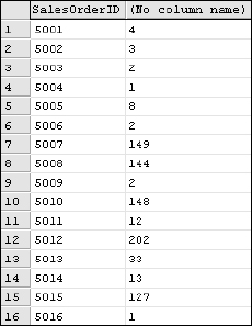
Figure 7-3

Because detail rows contain multiple quantities, you really can't tell if these rows are aggregated. To get a better view, add another column using the COUNT() function. Also add column aliases to label these values:

SELECT  SalesOrderID
      , SUM(OrderQty) As QtySum
      , COUNT(SalesOrderID) As DetailCount
FROM SalesOrderDetail
GROUP BY SalesOrderID

The result, shown in Figure 7-4, shows that all but two of the visible rows were grouped and the SUM() function was applied to the OrderQty column value.

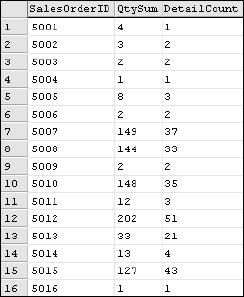
Figure 7-4

If you were to view the ungrouped records in this table, you could clearly see what's going on. The result shown in Figure 7-5 is just a simple SELECT query on the SalesOrderDetail table showing the first nine rows.

Figure 7-5

Sales order 5002 has two detail rows, whose OrderQty values add up to 3, order 5003 also has two detail rows with a total quantity of 3, and order 5005's quantity adds up to 8.

When grouping on more than one column, every unique combination of grouped values produces a row in the result set. Because the SalesOrderDetail table isn't preordered by the two columns you want to group on, you're explicitly ordering the results:

SELECT ProductID
     , SpecialOfferID
FROM SalesOrderDetail
GROUP BY ProductID, SpecialOfferID
ORDER BY ProductID, SpecialOfferID

The query returns a distinct list of ProductID and SpecialOfferID values (including null values), as shown in Figure 7-6.

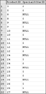
Figure 7-6

Although this may be interesting, it's not particularly useful information. Let's find out how many rows are actually being used to produce this list of distinct values. Extending the same query, add two columns that return the count of the ProductID and the SpecialOfferID values:

SELECT ProductID, COUNT(ProductID) As ProductIDCount
     , SpecialOfferID, COUNT(SpecialOfferID) As SpecialOfferIDCount
FROM SalesOrderDetail
GROUP BY  ProductID, SpecialOfferID
ORDER BY ProductID, SpecialOfferID

In the result set shown in Figure 7-7, you can see that you get the same rows.

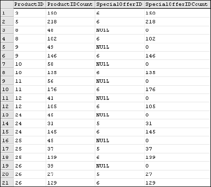
Figure 7-7

What you didn't see in the first result set is that the first row is an aggregation of 150 rows where the ProductID was 3 and the SpecialOfferID value was 6. The second row represents 218 rows. In the third row, 48 individual rows had a ProductID value of 8 and the SpecialOfferID was null. The COUNT() function returns 0 because null values are not considered in aggregate function calculations. 102 rows had the same ProductID value but the SpecialOfferID value was 6.

For a more real-world example, due to the complexity of the AdventureWorks database, it's necessary to create a fairly complex query with several table joins. Again, don't be concerned with the statements in the FROM clause, but do pay attention to the column list after the SELECT statement. You'll come back to this query in the next chapter.

The purpose of this query is to find out what products your customers have purchased. The Individual table contains personal information about human being–type customers (rather than stores that buy wholesale products). You've already seen that sales orders have order details, and a sales order detail line is related to a product:

SELECT
        Store.Name AS StoreName
      , Product.Name AS ProductName
      , COUNT(SalesOrderDetail.ProductID) AS PurchaseCount
FROM
      Customer INNER JOIN SalesOrderHeader
      ON Customer.CustomerID = SalesOrderHeader.CustomerID
      INNER JOIN SalesOrderDetail
      ON SalesOrderHeader.SalesOrderID = SalesOrderDetail.SalesOrderID
      INNER JOIN Product ON SalesOrderDetail.ProductID = Product.ProductID
      INNER JOIN Store ON Customer.CustomerID = Store.CustomerID
GROUP BY Product.Name, Store.Name
ORDER BY Store.Name, Product.Name

Three columns are returned from the query: the StoreName, the ProductName, and the number of product records in each group (PurchaseCount), using the COUNT() function. This returns the number of times a store purchased the same product. You could use the product Name in the COUNT() function but it's usually more efficient to use primary key columns. Note that even though the StoreName and ProductName columns are aliased in the SELECT list, when used in the GROUP BY and ORDER BY statements, the alias name is not used; only the qualified column names are used.

Figure 7-8 shows the first 34 rows in the result set.

Suppose that the purpose of this query was to locate stores that have purchased more than four of any product. Rather than scrolling through 20,531 rows, you can modify the query for rows with a count greater than four.

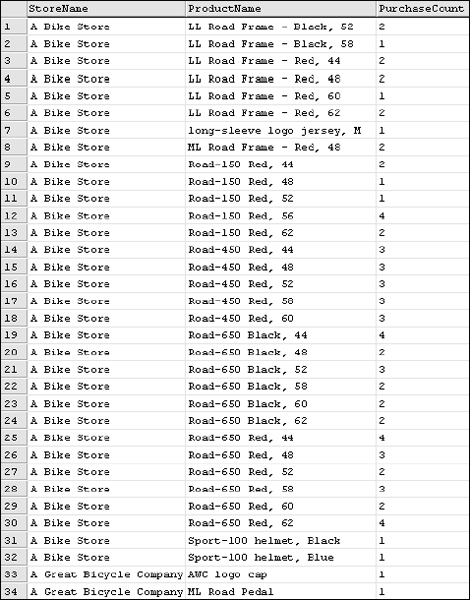
Figure 7-8

HAVING

How do you identify these rows? You can't use the WHERE clause because it is processed prior to grouping and aggregation; therefore, you need some way to filter the rows after the grouping has been completed. This is the job of the HAVING clause. The HAVING clause is limited to those columns and aggregate expressions that have already been specified on the SELECT statement. Typically, you will refer to aggregate values by simply repeating the aggregate function expression in the HAVING clause, just like you did in the SELECT statement. Here is the previous query with this expression added:

SELECT
        Store.Name AS StoreName
      , Product.Name AS ProductName
      , COUNT(SalesOrderDetail.ProductID) AS PurchaseCount
FROM
      Customer INNER JOIN SalesOrderHeader
      ON Customer.CustomerID = SalesOrderHeader.CustomerID
      INNER JOIN SalesOrderDetail
      ON SalesOrderHeader.SalesOrderID = SalesOrderDetail.SalesOrderID
      INNER JOIN Product ON SalesOrderDetail.ProductID = Product.ProductID
      INNER JOIN Store ON Customer.CustomerID = Store.CustomerID
GROUP BY Product.Name, Store.Name
HAVING COUNT(SalesOrderDetail.ProductID) > 4
ORDER BY Store.Name, Product.Name

The result set is now reduced to 2,139 rows, including only the store/product purchases. Examining the results shows something very interesting. In the previous results, you saw that there appeared to be a lot of transactions for the store called A Bike Store. However, when you look at the results in this way, you see that this customer purchased only small quantities of each product. As such, they are not included in these results, shown in Figure 7-9.

This data makes sense because most of the products listed with higher product counts are lower-priced items that tend to sell quickly.

The HAVING clause works much like the WHERE clause in that you can use any combination of comparison expressions and logical operators. Just be mindful that it is processed after the initial record selection (which is filtered by the WHERE clause) and that you are limited to the columns and aggregate expressions in the SELECT statement.

I'll use an example from the AdventureWorks database so you can follow along and work with the data yourself. Chapter 3 pointed out that the SQL Server Product Team had some fun putting the Employee sample data together. You'll see some more evidence of this. I thought it would be fun to see what gender variations there were for first names such as Terry and Pat. It turns out that our friends at Microsoft took this a little further.

Grouping the Employee table on the FirstName and Gender columns will return all the combinations of these values. I'll aggregate the EmployeeID column using the COUNT() function so you can see how many records there are for each FirstName/Gender combination. Here's the SQL expression for this query:

SELECT FirstName, Gender, COUNT(EmployeeID)
FROM Employee
GROUP BY  FirstName, Gender
ORDER BY FirstName, Gender

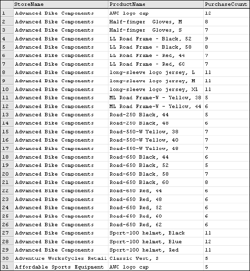
Figure 7-9

I've scrolled down a bit to view some of the rows with a higher count. In Figure 7-10, you can see that there are some interesting anomalies in the results. Of the four employees named Brian, three of them are female.

I can't be certain but I think that some of the folks on the SQL Server product team intended for this to be an inside joke and probably wondered if anyone would notice (considering that some of the names in this table are actual product team members). There are also five female employees named David. Apparently someone has a sense humor.

Totals and Subtotals

Before getting into a discussion about the techniques available for totaling grouped aggregates and creating subtotal breaks, a discussion of how you will use this data is needed. SQL Server is typically used as the back-end data store for some type of application or data consumer product. Many data presentation and reporting tools exist that will take care of formatting and totaling values from your queries. The technique you choose will largely depend on the tool or application that will consume this data. A number of products in the Microsoft suite can be used to easily present query results in a readable form. These include Excel, Access, and SQL Server Reporting Services.

Figure 7-10

One important consideration is whether you want the data to be grouped, aggregated, and subtotaled by the database server or by the client application after results have been returned from the database. There is little doubt that it is more efficient to let the database server do the work and send less data across the network. However, consider the case where an application allows users to interact with data, choosing different sorting and grouping options. It might make more sense to send raw data to the application one time so it can be manipulated by the client rather than refreshing the result set and resending a different result each time the user chooses a grouping or sorting option. These are decisions that you and solutions designers might need to make on a larger scale. The purpose here is to discuss the options in SQL Server to do the grouping and subtotaling at the database server.

When I use the terms totaling and subtotaling, I use these in a general sense to mean applying whatever aggregate functions you choose at various group levels. So, for example, if I were using the AVG() function to return the average purchase price per product, and per quarter at the quarter level, I would want to see the average calculation for all of the product price averages. I'm loosely using the term subtotal, even though I expect to see an average calculation rather than a sum or total.

Subgrouping

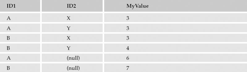
With more than one column referenced in the GROUP BY clause, some interesting things happen. For the sake of simplicity, a hypothetical table follows with simplified values.

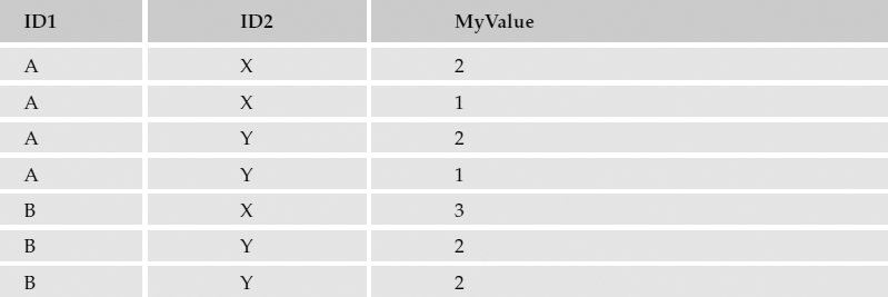
In a query for my hypothetical table, I include the first two columns, ID1 and ID2, in the GROUP BY clause and use the SUM() function to total the values in the third column:

SELECT ID1, ID2, Sum(MyValue)
FROM MyFakeTable
GROUP BY ID1, ID2

Multiple rows are returned, one for each unique combination of values, as shown in the following table.

What I don't have in this result set is the sum for all occurrences where ID1 is equal to A or where ID2 is equal to Y. To get the aggregate result of a grouped query, you can use the ROLLUP and CUBE statements. These will essentially take the results from the grouped query and apply the same aggregation to either the first column's values or all combinations of values for each column that appears in the GROUP BY column list.

WITH ROLLUP

This is the simplest option for calculating subtotals and totals on the first column in the GROUP BY column list. In the case of my hypothetical example, in addition to calculating the sum of each unique column value, totals would be tallied for the value A and B in the ID1 column only. Using the same query, I've added WITH ROLLUP after the GROUP BY statement:

SELECT ID1, ID2, SUM(MyValue)
FROM MyFakeTable
GROUP BY ID1, ID2
WITH ROLLUP

The results would look something like those shown in the following table.

Null values are used to indicate that the corresponding column was ignored when calculating the aggregate value.

WITH CUBE

The CUBE operator is an expanded version of the ROLLUP operator. Rather than just rolling up the aggregate values for the first column in the GROUP BY list, CUBE performs this rollup for every combination of grouped column values. In the case of the hypothetical tables used in the previous example, three additional rows are added to the result set. Here is the same query using WITH CUBE rather than WITH ROLLUP:

SELECT ID1, ID2, SUM(MyValue)
FROM MyFakeTable
GROUP BY ID1, ID2
WITH CUBE

The corresponding result set is shown in the following table.

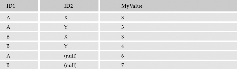
Null values in the first column indicate that this is a rollup on the values in the second column. In this case, these rows contain subtotal values for all rows where ID2 is equal to X or Y. The last row has null values in both grouped columns. This indicates that it is a grand total, the sum of all rows. Be advised that CUBE operations are expensive when it comes to server resources. Carefully consider whether it would be more efficient to just send the simplified aggregate data to the application and let it do the equivalent operations to derive the cubed data.

The GROUPING() Function

Let's go back to the AdventureWorks Product table example used earlier. I made a point not to use this table for the ROLLUP and CUBE examples because it would throw a wrench into the works. Go back and take another look at Figure 7-7; note the null values in the SpecialOfferID column. You'll recall that when using the ROLLUP and CUBE operators, a null is used to indicate a rollup or subtotal row where that column's value isn't being considered. What if a column in the GROUP BY list actually contains null values? Here's the earlier example again, with the added ROLLUP operator:

SELECT ProductID, COUNT(ProductID) As ProductIDCount
     , SpecialOfferID, COUNT(SpecialOfferID) As SpecialOfferIDCount
FROM SalesOrderDetail
GROUP BY ProductID, SpecialOfferID
WITH ROLLUP
ORDER BY ProductID, SpecialOfferID

In the result set shown in Figure 7-11, additional rows are added with subtotals.

Figure 7-11

Take a close look at rows 6, 7, and 8. Which one contains the subtotal for all products where the ProductID is 8? Two rows have nulls in the SpecialOfferID column. One of them contains NULL because some of this column's values are, in fact, NULL. The answer is row 7, because the count of the ProductID is higher than any other. Row 6 has a SpecialOfferID count of 0 because this row represents those rows where the SpecialOfferID is actually NULL. Do you find this confusing? It certainly can be. Imagine the added confusion if you were grouping on more than two columns, or using the CUBE operator rather than ROLLUP. Imagine taking the results of this query to your software developer and asking him to create a custom report with subtotals and totals and then try to explain this grouping criterion. This is where the GROUPING() function comes in.

The GROUPING() function returns a bit value (1 or 0) to indicate that a row is a rollup. This makes it easy to separate the aggregation of null values. Any application or tool that consumes grouped data can easily distinguish the rolled-up subtotal rows from simple grouped rows. Here's the query with two columns added using the GROUPING() function:

SELECT ProductID
     , GROUPING(ProductID) As ProdGroup
     , COUNT(ProductID) As ProductIDCount
     , SpecialOfferID
     , GROUPING(SpecialOfferID) As SO_Group
     , COUNT(SpecialOfferID) As SpecialOfferIDCount
FROM SalesOrderDetail
GROUP BY ProductID, SpecialOfferID
WITH ROLLUP
ORDER BY ProductID, SpecialOfferID

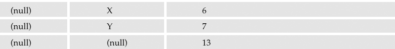
In the results shown in Figure 7-12, you can see the two new columns (aliased as ProdGroup and SO_Group). The first row in the result set is the grand total, with rolled-up values for all rows (any combination of ProductID and SpecialOfferID values). This row and each individual rollup row is also flagged with a 1.

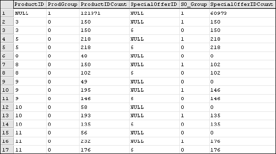
Figure 7-12

Because this is a ROLLUP query, only the SpecialOfferID values get rolled up into their respective ProductID combination counterparts. If you substitute CUBE for the ROLLUP function, you will see additional Grouping flags for the ProductID.

Note that if the results of these grouped and aggregated queries will be fed to a custom reporting solution or a similar application, application developers will appreciate the output from the GROUPING() function. This can make life much easier for a custom software developer or report designer.

COMPUTE and COMPUTE BY

Regardless of the data you might work with, SQL Server was designed, and is optimized, to return rows and columns—two dimensions. Likewise, software designed to consume SQL data expects to receive two-dimensional data. All of the components, application programming interfaces (APIs), and connection utilities are engineered to work with two-dimensional result sets.

Why am I making such a big deal out of this two-dimensional result set business? The COMPUTE clause is a very simple means for viewing data with totals and subtotals, but it breaks all the rules when it comes to standard results. It's also important to note that this is a proprietary SQL Server feature and isn't recognized by the ANSI SQL specification. My purpose is not to try to talk you out of using these features entirely but to realize its limitations. This is an effective technique for viewing summary data, but its usefulness may be somewhat limited in many real software solutions because it does not return data in a format that is consumable by any application. Its usefulness is limited to Query Analyzer or SQL Server Management Studio.

Suppose that the sales manager calls you on the phone and asks you to tell her what the total sales were for last month. She doesn't need a formal report, and you're not going to develop a custom application for users to do this themselves. She just wants a list of sales orders with the total. Using this technique may be the best choice.

Here's a simple example of the COMPUTE clause:

SELECT ProductID, SalesOrderID, OrderQty
FROM SalesOrderDetail
ORDER BY ProductID, SalesOrderID
COMPUTE SUM(OrderQty)

The query editor splits the result into two grids because the result doesn't fit into a standard two-dimensional grid, as shown in Figure 7-13.

I had asked for SQL Server to compute the sum of the OrderQty for the entire result set. This created a grand total for the entire range of data. Because of the formatting restrictions of viewing results in grid view, I'd like to show you the same result in text view.

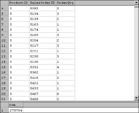
Figure 7-13

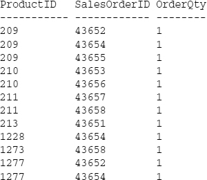
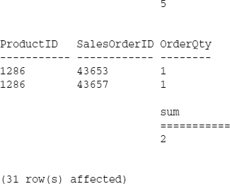
SELECT ProductID, SalesOrderID, OrderQty
FROM SalesOrderDetail
WHERE SalesOrderID > 43650
ORDER BY ProductID, SalesOrderID
COMPUTE SUM(OrderQty) By ProductID

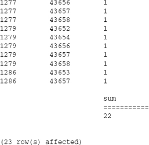
SELECT ProductID, SalesOrderID, OrderQty
FROM SalesOrderDetail
WHERE SalesOrderID > 43650
ORDER BY ProductID, SalesOrderID
COMPUTE SUM(OrderQty) By ProductID

Summary

This chapter introduced nine aggregate functions that can be used in a simple SELECT statement to return summary values for the entire range or with the GROUP BY clause to roll up groups of rows with similar values. The aggregate functions include simple mathematical operations, such as Count and Sum, and statistical functions such as variance and standard deviation.

The GROUP BY clause can be used to reduce the results of a query to distinct combinations of grouped values. When used with aggregate functions, this produces value summaries within the grouping.

The ROLLUP and CUBE statements extend grouping functionality by adding summary rows. Adding WITH ROLLUP to a grouped query will produce summary rows for the first column in the GROUP BY list. Adding WITH CUBE will add summary rows for every possible combination of grouped column values. The GROUPING() function can be used along with these operators to flag summary rows and to avoid confusion.

Use the COMPUTE statement sparingly and only for quick reports in Query Analyzer or the Query Editor. Although it's simple compared to using some of the other techniques discussed in this chapter, it is not ANSI SQL compliant and doesn't work with most software and programming tools. It is, however, a convenient method for viewing summary information quickly.

Exercises

Exercise 1

Write a query to return the first name and the highest ShiftID value for each group of employees named Kevin, Linda, or Mary.

Exercise 2

Return a list of ProductSubCategoryID values from the Product table. Include only subcategories that occur more than 20 times. In addition to the ID value, also return the first product name in alphabetical order and the highest price for products in this subcategory.

Exercise 3

Produce a list of managers from the Employee table using the ManagerID. For each manager, include the average base pay for all employees of each gender. Also include a row for each manager that includes the average base pay for all employees of that manager. This should be done using only one SELECT expression.