Chapter Nine. Priority Queues and Heapsort
Many applications require that we process records with keys in order, but not necessarily in full sorted order and not necessarily all at once. Often, we collect a set of records, then process the one with the largest key, then perhaps collect more records, then process the one with the current largest key, and so forth. An appropriate data structure in such an environment supports the operations of inserting a new element and deleting the largest element. Such a data structure is called a priority queue. Using priority queues is similar to using queues (delete the oldest) and stacks (delete the newest), but implementing them efficiently is more challenging. The priority queue is the most important example of the generalized queue ADT that we discussed in Section 4.6. In fact, the priority queue is a proper generalization of the stack and the queue, because we can implement these data structures with priority queues, using appropriate priority assignments (see Exercises 9.3 and 9.4).
Definition 9.1 A priority queue is a data structure of items with keys that supports two basic operations: insert a new item, and delete the item with the largest key.
Applications of priority queues include simulation systems, where the keys might correspond to event times, to be processed in chronological order; job scheduling in computer systems, where the keys might correspond to priorities indicating which users are to be served first; and numerical computations, where the keys might be computational errors, indicating that the largest should be dealt with first.
We can use any priority queue as the basis for a sorting algorithm by inserting all the records, then successively removing the largest to get the records in reverse order. Later on in this book, we shall see how to use priority queues as building blocks for more advanced algorithms. In Part 5, we shall develop a file-compression algorithm using routines from this chapter; and in Part 7, we shall see how priority queues are an appropriate abstraction for helping us understand the relationships among several fundamental graph-searching algorithms. These are but a few examples of the important role played by the priority queue as a basic tool in algorithm design.
In practice, priority queues are more complex than the simple definition just given, because there are several other operations that we may need to perform to maintain them under all the conditions that might arise when we are using them. Indeed, one of the main reasons that many priority queue implementations are so useful is their flexibility in allowing client application programs to perform a variety of different operations on sets of records with keys. We want to build and maintain a data structure containing records with numerical keys (priorities) that supports some of the following operations:
• Construct a priority queue from N given items.
• Insert a new item.
• Delete the maximum item.
• Change the priority of an arbitrary specified item.
• Delete an arbitrary specified item.
• Join two priority queues into one large one.
If records can have duplicate keys, we take “maximum” to mean “any record with the largest key value.” As with many data structures, we also need to add standard initialize, test if empty, and perhaps destroy and copy operations to this set.
There is overlap among these operations, and it is sometimes convenient to define other, similar operations. For example, certain clients may need frequently to find the maximum item in the priority queue, without necessarily removing it. Or, we might have an operation to replace the maximum item with a new item. We could implement operations such as these using our two basic operations as building blocks: Find the maximum could be delete the maximum followed by insert, and replace the maximum could be either insert followed by delete the maximum or delete the maximum followed by insert. We normally get more efficient code, however, by implementing such operations directly, provided that they are needed and precisely specified. Precise specification is not always as straightforward as it might seem. For example, the two options just given for replace the maximum are quite different: the former always makes the priority queue grow temporarily by one item, and the latter always puts the new item on the queue. Similarly, the change priority operation could be implemented as a delete followed by an insert, and construct could be implemented with repeated uses of insert.
For some applications, it might be slightly more convenient to switch around to work with the minimum, rather than with the maximum. We stick primarily with priority queues that are oriented toward accessing the maximum key. When we do need the other kind, we shall refer to it (a priority queue that allows us to delete the minimum item) as a minimum-oriented priority queue.
The priority queue is a prototypical abstract data type (ADT) (see Chapter 4): It represents a well-defined set of operations on data, and it provides a convenient abstraction that allows us to separate applications programs (clients) from various implementations that we will consider in this chapter. The interface given in Program 9.1 defines the most basic priority-queue operations; we shall consider a more complete interface in Section 9.5. Strictly speaking, different subsets of the various operations that we might want to include lead to different abstract data structures, but the priority queue is essentially characterized by the delete-the-maximum and insert operations, so we shall focus on them.
Different implementations of priority queues afford different performance characteristics for the various operations to be performed, and different applications need efficient performance for different sets of operations. Indeed, performance differences are, in principle, the only differences that can arise in the abstract-data-type concept. This situation leads to cost tradeoffs. In this chapter, we consider a variety of ways of approaching these cost tradeoffs, nearly reaching the ideal of being able to perform the delete the maximum operation in logarithmic time and all the other operations in constant time.
First, we illustrate this point in Section 9.1 by discussing a few elementary data structures for implementing priority queues. Next, in Sections 9.2 through 9.4, we concentrate on a classical data structure called the heap, which allows efficient implementations of all the operations but join. We also look at an important sorting algorithm that follows naturally from these implementations, in Section 9.4. Following this, we look in more detail at some of the problems involved in developing complete priority-queue ADTs, in Sections 9.5 and 9.6. Finally, in Section 9.7, we examine a more advanced data structure, called the binomial queue, that we use to implement all the operations (including join) in worst-case logarithmic time.
During our study of all these various data structures, we shall bear in mind both the basic tradeoffs dictated by linked versus sequential memory allocation (as introduced in Chapter 3) and the problems involved with making packages usable by applications programs. In particular, some of the advanced algorithms that appear later in this book are client programs that make use of priority queues.
P R I O * R * * I * T * Y * * * Q U E * * * U * E.
Give the sequence of values returned by the delete the maximum operations.
![]() 9.2 Add to the conventions of Exercise 9.1 a plus sign to mean join and parentheses to delimit the priority queue created by the operations within them. Give the contents of the priority queue after the sequence
9.2 Add to the conventions of Exercise 9.1 a plus sign to mean join and parentheses to delimit the priority queue created by the operations within them. Give the contents of the priority queue after the sequence
( ( ( P R I O *) + ( R * I T * Y * ) ) * * * ) + ( Q U E * * * U * E ).
![]() 9.3 Explain how to use a priority queue ADT to implement a stack ADT.
9.3 Explain how to use a priority queue ADT to implement a stack ADT.
![]() 9.4 Explain how to use a priority queue ADT to implement a queue ADT.
9.4 Explain how to use a priority queue ADT to implement a queue ADT.
9.1 Elementary Implementations
The basic data structures that we discussed in Chapter 3 provide us with numerous options for implementing priority queues. Program 9.2 is an implementation that uses an unordered array as the underlying data structure. The find the maximum operation is implemented by scanning the array to find the maximum, then exchanging the maximum item with the last item and decrementing the queue size. Figure 9.1 shows the contents of the array for a sample sequence of operations. This basic implementation corresponds to similar implementations that we saw in Chapter 4 for stacks and queues (see Programs 4.4 and 4.11), and is useful for small queues. The significant difference has to do with performance. For stacks and queues, we were able to develop implementations of all the operations that take constant time; for priority queues, it is easy to find implementations where either the insert or the delete the maximum functions takes constant time, but finding an implementation where both operations will be fast is a more difficult task, and is the subject of this chapter.
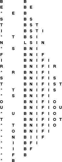
This sequence shows the result of the sequence of operations in the left column (top to bottom), where a letter denotes insert and an asterisk denotes delete the maximum. Each line displays the operation, the letter deleted for the delete-the-maximum operations, and the contents of the array after the operation.
Figure 9.1 Priority-queue example (unordered array representation)
We can use unordered or ordered sequences, implemented as linked lists or as arrays. The basic tradeoff between leaving the items unordered and keeping them in order is that maintaining an ordered sequence allows for constant-time delete the maximum and find the maximum but might mean going through the whole list for insert, whereas an unordered sequence allows a constant-time insert but might mean going through the whole sequence for delete the maximum and find the maximum. The unordered sequence is the prototypical lazy approach to this problem, where we defer doing work until necessary (to find the maximum); the ordered sequence is the prototypical eager approach to the problem, where we do as much work as we can up front (keep the list sorted on insertion) to make later operations efficient. We can use an array or linked-list representation in either case, with the basic tradeoff that the (doubly) linked list allows a constant-time delete (and, in the unordered case join), but requires more space for the links.
The worst-case costs of the various operations (within a constant factor) on a priority queue of size N for various implementations are summarized in Table 9.1.
Implementations of the priority queue ADT have widely varying performance characteristics, as indicated in this table of the worst-case time (within a constant factor for large N) for various methods. Elementary methods (first four lines) require constant time for some operations and linear time for others; more advanced methods guarantee logarithmic-or constant-time performance for most or all operations.
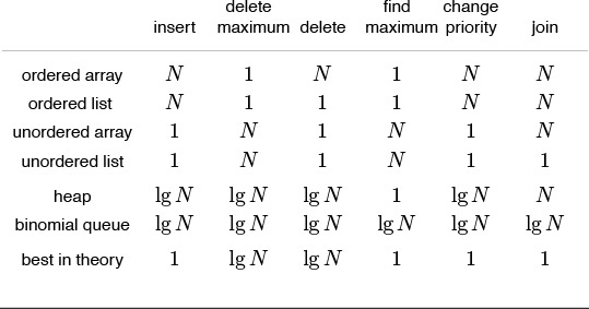
Table 9.1 Worst-case costs of priority queue operations
Developing a full implementation requires paying careful attention to the interface—particularly to how client programs access nodes for the delete and change priority operations, and how they access priority queues themselves as data types for the join operation. These issues are discussed in Sections 9.4 and 9.7, where two full implementations are given: one using doubly-linked unordered lists, and another using binomial queues.
The running time of a client program using priority queues depends not just on the keys, but also on the mix of the various operations. It is wise to keep in mind the simple implementations because they often can outperform more complicated methods in many practical situations. For example, the unordered-list implementation might be appropriate in an application where only a few delete the maximum operations are performed, as opposed to a huge number of insertions, whereas an ordered list would be appropriate if a huge number of find the maximum operations are involved, or if the items inserted tend to be larger than those already in the priority queue.
Exercises
![]() 9.5 Criticize the following idea: To implement find the maximum in constant time, why not keep track of the maximum value inserted so far, then return that value for find the maximum?
9.5 Criticize the following idea: To implement find the maximum in constant time, why not keep track of the maximum value inserted so far, then return that value for find the maximum?
![]() 9.6 Give the contents of the array after the execution of the sequence of operations depicted in Figure 9.1.
9.6 Give the contents of the array after the execution of the sequence of operations depicted in Figure 9.1.
9.7 Provide an implementation for the basic priority queue interface that uses an ordered array for the underlying data structure.
9.8 Provide an implementation for the basic priority queue interface that uses an unordered linked list for the underlying data structure. Hint: See Programs 4.5 and 4.10.
9.9 Provide an implementation for the basic priority queue interface that uses an ordered linked list for the underlying data structure. Hint: See Program 3.11.
![]() 9.10 Consider a lazy implementation where the list is ordered only when a delete the maximum or a find the maximum operation is performed. Insertions since the previous sort are kept on a separate list, then are sorted and merged in when necessary. Discuss advantages of such an implementation over the elementary implementations based on unordered and ordered lists.
9.10 Consider a lazy implementation where the list is ordered only when a delete the maximum or a find the maximum operation is performed. Insertions since the previous sort are kept on a separate list, then are sorted and merged in when necessary. Discuss advantages of such an implementation over the elementary implementations based on unordered and ordered lists.
![]() 9.11 Write a performance driver client program that uses
9.11 Write a performance driver client program that uses PQinsert to fill a priority queue, then uses PQdelmax to remove half the keys, then uses PQinsert to fill it up again, then uses PQdelmax to remove all the keys, doing so multiple times on random sequences of keys of various lengths ranging from small to large; measures the time taken for each run; and prints out or plots the average running times.
![]() 9.12 Write a performance driver client program that uses
9.12 Write a performance driver client program that uses PQinsert to fill a priority queue, then does as many PQdelmax and PQinsert operations as it can do in 1 second, doing so multiple times on random sequences of keys of various lengths ranging from small to large; and prints out or plots the average number of PQdelmax operations it was able to do.
9.13 Use your client program from Exercise 9.12 to compare the unordered-array implementation in Program 9.2 with your unordered-list implementation from Exercise 9.8.
9.14 Use your client program from Exercise 9.12 to compare your ordered-array and ordered-list implementations from Exercises 9.7 and 9.9.
![]() 9.15 Write an exercise driver client program that uses the functions in our priority-queue interface Program 9.1 on difficult or pathological cases that might turn up in practical applications. Simple examples include keys that are already in order, keys in reverse order, all keys the same, and sequences of keys having only two distinct values.
9.15 Write an exercise driver client program that uses the functions in our priority-queue interface Program 9.1 on difficult or pathological cases that might turn up in practical applications. Simple examples include keys that are already in order, keys in reverse order, all keys the same, and sequences of keys having only two distinct values.
9.16 (This exercise is 24 exercises in disguise.) Justify the worst-case bounds for the four elementary implementations that are given in Table 9.1, by reference to the implementation in Program 9.2 and your implementations from Exercises 9.7 through 9.9 for insert and delete the maximum; and by informally describing the methods for the other operations. For delete, change priority, and join, assume that you have a handle that gives you direct access to the referent.
9.2 Heap Data Structure
The main topic of this chapter is a simple data structure called the heap that can efficiently support the basic priority-queue operations. In a heap, the records are stored in an array such that each key is guaranteed to be larger than the keys at two other specific positions. In turn, each of those keys must be larger than two more keys, and so forth. This ordering is easy to see if we view the keys as being in a binary tree structure with edges from each key to the two keys known to be smaller.
Definition 9.2 A tree is heap-ordered if the key in each node is larger than or equal to the keys in all of that node’s children (if any). Equivalently, the key in each node of a heap-ordered tree is smaller than or equal to the key in that node’s parent (if any).
Property 9.1 No node in a heap-ordered tree has a key larger than the key at the root.
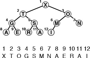
We could impose the heap-ordering restriction on any tree. It is particularly convenient, however, to use a complete binary tree. Recall from Chapter 3 that we can draw such a structure by placing the root node and then proceeding down the page and from left to right, connecting two nodes beneath each node on the previous level until N nodes have been placed. We can represent complete binary trees sequentially within an array by simply putting the root at position 1, its children at positions 2 and 3, the nodes at the next level in positions 4, 5, 6 and 7, and so on, as illustrated in Figure 9.2.
Considering the element in position ![]() i/2
i/2![]() in an array to be the parent of the element in position i, for 2 ≤ i ≤ N (or, equivalently, considering the ith element to be the parent of the 2ith element and the (2i + 1)st element), corresponds to a convenient representation of the elements as a tree. This correspondence is equivalent to numbering the nodes in a complete binary tree (with nodes on the bottom as far left as possible) in level order. A tree is heap-ordered if the key in any given node is greater than or equal to the keys of that node’s children. A heap is an array representation of a complete heap-ordered binary tree. The ith element in a heap is larger than or equal to both the 2ith and the (2i + 1)st elements.
in an array to be the parent of the element in position i, for 2 ≤ i ≤ N (or, equivalently, considering the ith element to be the parent of the 2ith element and the (2i + 1)st element), corresponds to a convenient representation of the elements as a tree. This correspondence is equivalent to numbering the nodes in a complete binary tree (with nodes on the bottom as far left as possible) in level order. A tree is heap-ordered if the key in any given node is greater than or equal to the keys of that node’s children. A heap is an array representation of a complete heap-ordered binary tree. The ith element in a heap is larger than or equal to both the 2ith and the (2i + 1)st elements.
Figure 9.2 Array representation of a heap-ordered complete binary tree
Definition 9.3 A heap is a set of nodes with keys arranged in a complete heap-ordered binary tree, represented as an array.
We could use a linked representation for heap-ordered trees, but complete trees provide us with the opportunity to use a compact array representation where we can easily get from a node to its parent and children without needing to maintain explicit links. The parent of the node in position i is in position ![]() i/2
i/2![]() , and, conversely, the two children of the node in position i are in positions 2i and 2i + 1. This arrangement makes traversal of such a tree even easier than if the tree were implemented with a linked representation, because, in a linked representation, we would need to have three links associated with each key to allow travel up and down the tree (each element would have one pointer to its parent and one to each child). Complete binary trees represented as arrays are rigid structures, but they have just enough flexibility to allow us to implement efficient priority-queue algorithms.
, and, conversely, the two children of the node in position i are in positions 2i and 2i + 1. This arrangement makes traversal of such a tree even easier than if the tree were implemented with a linked representation, because, in a linked representation, we would need to have three links associated with each key to allow travel up and down the tree (each element would have one pointer to its parent and one to each child). Complete binary trees represented as arrays are rigid structures, but they have just enough flexibility to allow us to implement efficient priority-queue algorithms.
We shall see in Section 9.3 that we can use heaps to implement all the priority queue operations (except join) such that they require logarithmic time in the worst case. The implementations all operate along some path inside the heap (moving from parent to child toward the bottom or from child to parent toward the top, but not switching directions). As we discussed in Chapter 3, all paths in a complete tree of N nodes have about lg N nodes on them: there are about N/2 nodes on the bottom, N/4 nodes with children on the bottom, N/8 nodes with grandchildren on the bottom, and so forth. Each generation has about one-half as many nodes as the next, and there are at most lg N generations.
We can also use explicit linked representations of tree structures to develop efficient implementations of the priority-queue operations. Examples include triply-linked heap-ordered complete trees (see Section 9.5), tournaments (see Program 5.19), and binomial queues (see Section 9.7). As with simple stacks and queues, one important reason to consider linked representations is that they free us from having to know the maximum queue size ahead of time, as is required with an array representation. We also can make use of the flexibility provided by linked structures to develop efficient algorithms, in certain situations. Readers who are inexperienced with using explicit tree structures are encouraged to read Chapter 12 to learn basic methods for the even more important symbol-table ADT implementation before tackling the linked tree representations discussed in the exercises in this chapter and in Section 9.7. However, careful consideration of linked structures can be reserved for a second reading, because our primary topic in this chapter is the heap (linkless array representation of the heap-ordered complete tree).
![]() 9.18 The largest element in a heap must appear in position 1, and the second largest element must be in position 2 or position 3. Give the list of positions in a heap of size 15 where the kth largest element (i) can appear, and (ii) cannot appear, for k = 2, 3, 4 (assuming the values to be distinct).
9.18 The largest element in a heap must appear in position 1, and the second largest element must be in position 2 or position 3. Give the list of positions in a heap of size 15 where the kth largest element (i) can appear, and (ii) cannot appear, for k = 2, 3, 4 (assuming the values to be distinct).
![]() 9.19 Answer Exercise 9.18 for general k, as a function of N, the heap size.
9.19 Answer Exercise 9.18 for general k, as a function of N, the heap size.
![]() 9.20 Answer Exercises 9.18 and 9.19 for the kth smallest element.
9.20 Answer Exercises 9.18 and 9.19 for the kth smallest element.
9.3 Algorithms on Heaps
The priority-queue algorithms on heaps all work by first making a simple modification that could violate the heap condition, then traveling through the heap, modifying the heap as required to ensure that the heap condition is satisfied everywhere. This process is sometimes called heapifying, or just fixing the heap. There are two cases. When the priority of some node is increased (or a new node is added at the bottom of a heap), we have to travel up the heap to restore the heap condition. When the priority of some node is decreased (for example, if we replace the node at the root with a new node), we have to travel down the heap to restore the heap condition. First, we consider how to implement these two basic functions; then, we see how to use them to implement the various priority-queue operations.
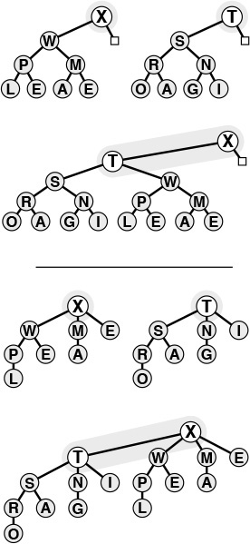
If the heap property is violated because a node’s key becomes larger than that node’s parent’s key, then we can make progress toward fixing the violation by exchanging the node with its parent. After the exchange, the node is larger than both its children (one is the old parent, the other is smaller than the old parent because it was a child of that node) but may be still be larger than its parent. We can fix that violation in the same way, and so forth, moving up the heap until we reach a node with larger key, or the root. An example of this process is shown in Figure 9.3. The code is straightforward, based on the notion that the parent of the node at position k in a heap is at position k/2. Program 9.3 is an implementation of a function that restores a possible violation due to increased priority at a given node in a heap by moving up the heap.
The tree depicted on the top is heap-ordered except for the node T on the bottom level. If we exchange T with its parent, the tree is heap-ordered, except possibly that T may be larger than its new parent. Continuing to exchange T with its parent until we encounter the root or a node on the path from T to the root that is larger than T, we can establish the heap condition for the whole tree. We can use this procedure as the basis for the insert operation on heaps, to reestablish the heap condition after adding a new element to a heap (at the rightmost position on the bottom level, starting a new level if necessary).
Figure 9.3 Bottom-up heapify
If the heap property is violated because a node’s key becomes smaller than one or both of that node’s childrens’ keys, then we can make progress toward fixing the violation by exchanging the node with the larger of its two children. This switch may cause a violation at the child; we fix that violation in the same way, and so forth, moving down the heap until we reach a node with both children smaller, or the bottom. An example of this process is shown in Figure 9.4. The code again follows directly from the fact that the children of the node at position k in a heap are at positions 2k and 2k+1. Program 9.4 is an implementation of a function that restores a possible violation due to increased priority at a given node in a heap by moving down the heap. This function needs to know the size of the heap (N) in order to be able to test when it has reached the bottom.

The tree depicted on the top is heap-ordered, except at the root. If we exchange the O with the larger of its two children (X), the tree is heap-ordered, except at the subtree rooted at O. Continuing to exchange O with the larger of its two children until we reach the bottom of the heap or a point where O is larger than both its children, we can establish the heap condition for the whole tree. We can use this procedure as the basis for the delete the maximum operation on heaps, to reestablish the heap condition after replacing the key at the root with the rightmost key on the bottom level.
Figure 9.4 Top-down heapify
These two operations are independent of the way that the tree structure is represented, as long as we can access the parent (for the bottom-up method) and the children (for the top-down method) of any node. For the bottom-up method, we move up the tree, exchanging the key in the given node with the key in its parent until we reach the root or a parent with a larger (or equal) key. For the top-down method, we move down the tree, exchanging the key in the given node with the largest key among that node’s children, moving down to that child, and continuing down the tree until we reach the bottom or a point where no child has a larger key. Generalized in this way, these operations apply not just to complete binary trees, but also to any tree structure. Advanced priority-queue algorithms usually use more general tree structures, but rely on these same basic operations to maintain access to the largest key in the structure, at the top.
If we imagine the heap to represent a corporate hierarchy, with each of the children of a node representing subordinates (and the parent representing the immediate superior), then these operations have amusing interpretations. The bottom-up method corresponds to a promising new manager arriving on the scene, being promoted up the chain of command (by exchanging jobs with any lower-qualified boss) until the new person encounters a higher-qualified boss. The top-down method is analogous to the situation when the president of the company is replaced by someone less qualified. If the president’s most powerful subordinate is stronger than the new person, they exchange jobs, and we move down the chain of command, demoting the new person and promoting others until the level of competence of the new person is reached, where there is no higher-qualified subordinate (this idealized scenario is rarely seen in the real world). Drawing on this analogy, we often refer to a movement up a heap as a promotion.
These two basic operations allow efficient implementation of the basic priority-queue ADT, as given in Program 9.5. With the priority queue represented as a heap-ordered array, using the insert operation amounts to adding the new element at the end and moving that element up through the heap to restore the heap condition; the delete the maximum operation amounts to taking the largest value off the top, then putting in the item from the end of the heap at the top and moving it down through the array to restore the heap condition.
Property 9.2 The insert and delete the maximum operations for the priority queue abstract data type can be implemented with heap-ordered trees such that insert requires no more than lg N comparisons and delete the maximum no more than 2lgN comparisons, when performed on an N-item queue.
Both operations involve moving along a path between the root and the bottom of the heap, and no path in a heap of size N includes more than lg N elements (see, for example, Property 5.8 and Exercise 5.77). The delete the maximum operation requires two comparisons for each node: one to find the child with the larger key, the other to decide whether that child needs to be promoted. ![]()
Figures 9.5 and 9.6 show an example in which we construct a heap by inserting items one by one into an initially empty heap. In the array representation that we have been using, this process corresponds to heap ordering the array by moving sequentially through the array, considering the size of the heap to grow by 1 each time that we move to a new item, and using fixUp to restore the heap order. The process takes time proportional to N log N in the worst case (if each new item is the largest seen so far, it travels all the way up the heap), but it turns out to take only linear time on the average (a random new item tends to travel up only a few levels). In Section 9.4 we shall see a way to construct a heap (to heap order an array) in linear worst-case time.
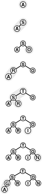
This sequence depicts the insertion of the keys A S O R T I N G into an initially empty heap. New items are added to the heap at the bottom, moving from left to right on the bottom level. Each insertion affects only the nodes on the path between the insertion point and the root, so the cost is proportional to the logarithm of the size of the heap in the worst case.
Figure 9.5 Top-down heap construction
This sequence depicts insertion of the keys E X A M P L E into the heap started in Figure 9.5. The total cost of constructing a heap of size N is less than
lg 1 + lg 2 + ... + lg N, which is less than N lg N.
Figure 9.6 Top-down heap construction (continued)
The basic fixUp and fixDown operations in Programs 9.3 and 9.4 also allow direct implementation for the change priority and delete operations. To change the priority of an item somewhere in the middle of the heap, we use fixUp to move up the heap if the priority is increased, and fixDown to go down the heap if the priority is decreased. Full implementations of such operations, which refer to specific data items, make sense only if a reference is maintained for each item to that item’s place in the data structure. We shall consider implementations that do so in detail in Sections 9.5 through 9.7.
Property 9.3 The change priority, delete, and replace the maximum operations for the priority queue abstract data type can be implemented with heap-ordered trees such that no more than 2 lgN comparisons are required for any operation on an N-item queue.
Since they require handles to items, we defer considering implementations that support these operations to Section 9.6 (see Program 9.12 and Figure 9.14). They all involve moving along one path in the heap, perhaps from top to bottom or bottom to top in the worst case. ![]()
Note carefully that the join operation is not included on this list. Combining two priority queues efficiently seems to require a much more sophisticated data structure. We shall consider such a data structure in detail in Section 9.7. Otherwise, the simple heap-based method given here suffices for a broad variety of applications. It uses minimal extra space and is guaranteed to run efficiently except in the presence of frequent and large join operations.
As we have mentioned, we can use any priority queue to develop a sorting method, as shown in Program 9.6. We simply insert all the keys to be sorted into the priority queue, then repeatedly use delete the maximum to remove them all in decreasing order. Using a priority queue represented as an unordered list in this way corresponds to doing a selection sort; using an ordered list corresponds to doing an insertion sort.
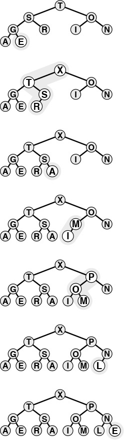
Figures 9.5 and 9.6 give an example of the first phase (the construction process) when a heap-based priority-queue implementation is used; Figures 9.7 and 9.8 show the second phase (which we refer to as the sortdown process) for the heap-based implementation. For practical purposes, this method is comparatively inelegant, because it unnecessarily makes an extra copy of the items to be sorted (in the priority queue). Also, using N successive insertions is not the most efficient way to build a heap from N given elements. In the next section, we address these two points as we consider an implementation of the classical heapsort algorithm.
After replacing the largest element in the heap by the rightmost element on the bottom level, we can restore the heap order by sifting down along a path from the root to the bottom.
Figure 9.7 Sorting from a heap
This sequence depicts removal of the rest of the keys from the heap in Figure 9.7. Even if every element goes all the way back to the bottom, the total cost of the sorting phase is less than
lg N + ... + lg2 + lg1, which is less than N log N.
Figure 9.8 Sorting from a heap (continued)
Exercises
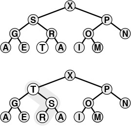
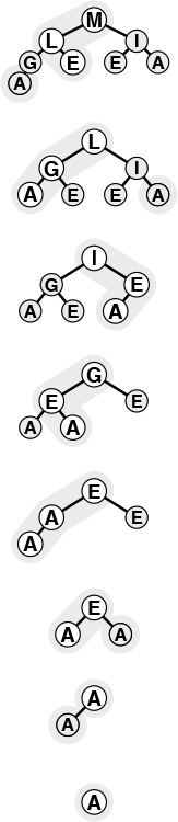
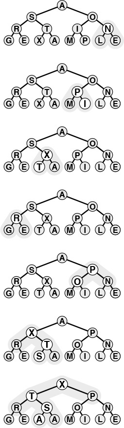
![]() 9.21 Give the heap that results when the keys E A S Y Q U E S T I O N are inserted into an initially empty heap.
9.21 Give the heap that results when the keys E A S Y Q U E S T I O N are inserted into an initially empty heap.
![]() 9.22 Using the conventions of Exercise 9.1 give the sequence of heaps produced when the operations
9.22 Using the conventions of Exercise 9.1 give the sequence of heaps produced when the operations
P R I O * R * * I * T * Y * * * Q U E * * * U * E
are performed on an initially empty heap.
9.23 Because the exch primitive is used in the heapify operations, the items are loaded and stored twice as often as necessary. Give more efficient implementations that avoid this problem, a la insertion sort.
9.24 Why do we not use a sentinel to avoid the j<N test in fixDown?
![]() 9.25 Add the replace the maximum operation to the heap-based priority-queue implementation of Program 9.5. Be sure to consider the case when the value to be added is larger than all values in the queue. Note: Use of
9.25 Add the replace the maximum operation to the heap-based priority-queue implementation of Program 9.5. Be sure to consider the case when the value to be added is larger than all values in the queue. Note: Use of pq[0] leads to an elegant solution.
9.26 What is the minimum number of keys that must be moved during a delete the maximum operation in a heap? Give a heap of size 15 for which the minimum is achieved.
9.27 What is the minimum number of keys that must be moved during three successive delete the maximum operations in a heap? Give a heap of size 15 for which the minimum is achieved.
9.4 Heapsort
We can adapt the basic idea in Program 9.6 to sort an array without needing any extra space, by maintaining the heap within the array to be sorted. That is, focusing on the task of sorting, we abandon the notion of hiding the representation of the priority queue, and rather than being constrained by the interface to the priority-queue ADT, we use fixUp and fixDown directly.
Using Program 9.5 directly in Program 9.6 corresponds to proceeding from left to right through the array, using fixUp to ensure that the elements to the left of the scanning pointer make up a heap-ordered complete tree. Then, during the sortdown process, we put the largest element into the place vacated as the heap shrinks. That is, the sortdown process is like selection sort, but it uses a more efficient way to find the largest element in the unsorted part of the array.
Rather than constructing the heap via successive insertions as shown in Figures 9.5 and 9.6, it is more efficient to build the heap by going backward through it, making little subheaps from the bottom up, as shown in Figure 9.9. That is, we view every position in the array as the root of a small subheap, and take advantage of the fact that fixDown works as well for such subheaps as it does for the big heap. If the two children of a node are heaps, then calling fixDown on that node makes the subtree rooted there a heap. By working backward through the heap, calling fixDown on each node, we can establish the heap property inductively. The scan starts halfway back through the array because we can skip the subheaps of size 1.
Working from right to left and bottom to top, we construct a heap by ensuring that the subtree below the current node is heap ordered. The total cost is linear in the worst case, because most nodes are near the bottom.
Figure 9.9 Bottom-up heap construction
A full implementation is given in Program 9.7, the classical heapsort algorithm. Although the loops in this program seem to do different tasks (the first constructs the heap, and the second destroys the heap for the sortdown), they are built around the same fundamental procedure, which restores order in a tree that is heap-ordered except possibly at the root, using the array representation of a complete tree. Figure 9.10 illustrates the contents of the array for the example corresponding to Figures 9.7 through 9.9.
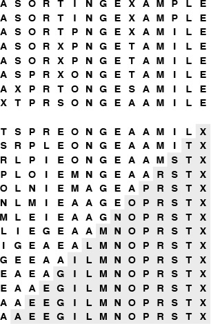
Heapsort is an efficient selection-based algorithm. First, we build a heap from the bottom up, in-place. The top eight lines in this figure correspond to Figure 9.9. Next, we repeatedly remove the largest element in the heap. The unshaded parts of the bottom lines correspond to Figures 9.7 and 9.8; the shaded parts contain the growing sorted file.
Figure 9.10 Heapsort example
Property 9.4 Bottom-up heap construction takes linear time.
This fact follows from the observation that most of the heaps processed are small. For example, to build a heap of 127 elements, we process 32 heaps of size 3, 16 heaps of size 7, 8 heaps of size 15, 4 heaps of size 31, 2 heaps of size 63, and 1 heap of size 127, so 32 · 1 + 16 · 2 + 8 · 3 + 4 · 4 + 2 · 5 + 1 · 6 = 120 promotions (twice as many comparisons) are required in the worst case. For N = 2n – 1, an upper bound on the number of promotions is
A similar proof holds when N +1 is not a power of 2. ![]()
This property is not of particular importance for heapsort, because its time is still dominated by the N log N time for the sortdown, but it is important for other priority-queue applications, where a linear-time construct operation can lead to a linear-time algorithm. As noted in Figure 9.6, constructing a heap with N successive insert operations requires a total of N log N steps in the worst case (even though the total turns out to be linear on the average for random files).
Property 9.5 Heapsort uses fewer than 2N lg N comparisons to sort N elements.
The slightly higher bound 3N lg N follows immediately from Property 9.2. The bound given here follows from a more careful count based on Property 9.4. ![]()
Property 9.5 and the in-place property are the two primary reasons that heapsort is of practical interest: It is guaranteed to sort N elements in place in time proportional to N log N, no matter what the input. There is no worst-case input that makes heapsort run significantly slower (unlike quicksort), and heapsort does not use any extra space (unlike mergesort). This guaranteed worst-case performance does come at a price: for example, the algorithm’s inner loop (cost per comparison) has more basic operations than quicksort’s, and it uses more comparisons than quicksort for random files, so heapsort is likely to be slower than quicksort for typical or random files.
Heaps are also useful for solving the selection problem of finding the k largest of N items (see Chapter 7), particularly if k is small. We simply stop the heapsort algorithm after k items have been taken from the top of the heap.
Property 9.6 Heap-based selection allows the kth largest of N items to be found in time proportional to N when k is small or close to N, and in time proportional to N log N otherwise.
One option is to build a heap, using fewer than 2N comparisons (by Property 9.4), then to remove the k largest elements, using 2k lg N or fewer comparisons (by Property 9.2), for a total of 2N + 2k lg N. Another method is to build a minimum-oriented heap of size k, then to perform k replace the minimum (insert followed by delete the minimum) operations with the remaining elements for a total of at most 2k + 2(N – k)lg k comparisons (see Exercise 9.35). This method uses space proportional to k, so is attractive for finding the k largest of N elements when k is small and N is large (or is not known in advance). For random keys and other typical situations, the lg k upper bound for heap operations in the second method is likely to be O(1) when k is small relative to N (see Exercise 9.36). ![]()
Various ways to improve heapsort further have been investigated. One idea, developed by Floyd, is to note that an element reinserted into the heap during the sortdown process usually goes all the way to the bottom, so we can save time by avoiding the check for whether the element has reached its position, simply promoting the larger of the two children until the bottom is reached, then moving back up the heap to the proper position. This idea cuts the number of comparisons by a factor of 2 asymptotically—close to the lg N! ≈ N lg N –N/ ln 2 that is the absolute minimum number of comparisons needed by any sorting algorithm (see Part 8). The method requires extra bookkeeping, and it is useful in practice only when the cost of comparisons is relatively high (for example, when we are sorting records with strings or other types of long keys).
Another idea is to build heaps based on an array representation of complete heap-ordered ternary trees, with a node at position k larger than or equal to nodes at positions 3k – 1, 3k, and 3k + 1 and smaller than or equal to nodes at position ![]() (k + 1)/3
(k + 1)/3![]() , for positions between 1 and N in an array of N elements. There is a tradeoff between the lower cost from the reduced tree height and the higher cost of finding the largest of the three children at each node. This tradeoff is dependent on details of the implementation (see Exercise 9.30). Further increasing the number of children per node is not likely to be productive.
, for positions between 1 and N in an array of N elements. There is a tradeoff between the lower cost from the reduced tree height and the higher cost of finding the largest of the three children at each node. This tradeoff is dependent on details of the implementation (see Exercise 9.30). Further increasing the number of children per node is not likely to be productive.
Figure 9.11 shows heapsort in operation on a randomly ordered file. At first, the process seems to do anything but sorting, because large elements are moving to the beginning of the file as the heap is being constructed. But then the method looks more like a mirror image of selection sort, as expected. Figure 9.12 shows that different types of input files can yield heaps with peculiar characteristics, but they look more like random heaps as the sort progresses.
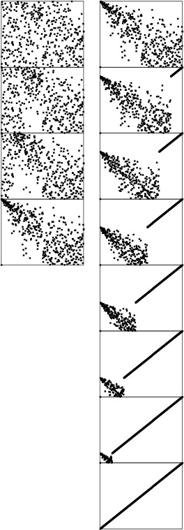
The construction process (left) seems to unsort the file, putting large elements near the beginning. Then, the sortdown process (right) works like selection sort, keeping a heap at the beginning and building up the sorted array at the end of the file.
Figure 9.11 Dynamic characteristics of heapsort
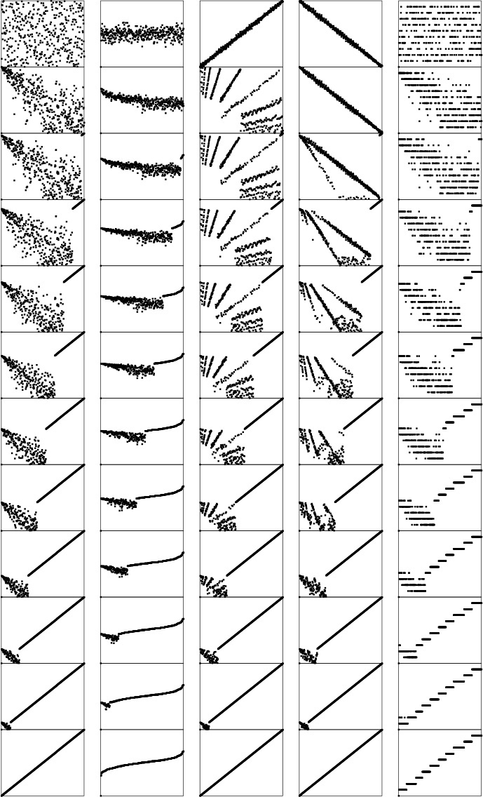
The running time for heapsort is not particularly sensitive to the input. No matter what the input values are, the largest element is always found in less than lg N steps. These diagrams show files that are random, Gaussian, nearly ordered, nearly reverse-ordered, and randomly ordered with 10 distinct key values (at the top, left to right). The second diagrams from the top show the heap constructed by the bottom-up algorithm, and the remaining diagrams show the sortdown process for each file. The heaps somewhat mirror the initial file at the beginning, but all become more like the heaps for a random file as the process continues.
Figure 9.12 Dynamic characteristics of heapsort on various types of files
Naturally, we are interested in the issue of how to choose among heapsort, quicksort, and mergesort for a particular application. The choice between heapsort and mergesort essentially reduces to a choice between a sort that is not stable (see Exercise 9.28) and one that uses extra memory; the choice between heapsort and quicksort reduces to a choice between average-case speed and worst-case speed. Having dealt extensively with improving the inner loops of quicksort and mergesort, we leave this activity for heapsort as exercises in this chapter. Making heapsort faster than quicksort is typically not in the cards—as indicated by the empirical studies in Table 9.2—but people interested in fast sorts on their machines will find the exercise instructive. As usual, various specific properties of machines and programming environments can play an important role. For example, quicksort and mergesort have a locality property that gives them a further advantage on certain machines. When comparisons are extremely expensive, Floyd’s version is the method of choice, as it is nearly optimal in terms of time and space costs in such situations.
The relative timings for various sorts on files of random integers in the left part of the table confirm our expectations from the lengths of the inner loops that heapsort is slower than quicksort but competitive with mergesort. The timings for the first N words of Moby Dick in the right part of the table show that Floyd’s method is an effective improvement to heapsort when comparisons are expensive.
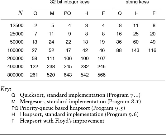
Table 9.2 Empirical study of heapsort algorithms
![]() 9.29 Empirically determine the percentage of time heapsort spends in the construction phase for N = 103, 104, 105, and 106.
9.29 Empirically determine the percentage of time heapsort spends in the construction phase for N = 103, 104, 105, and 106.
![]() 9.30 Implement a version of heapsort based on complete heap-ordered ternary trees, as described in the text. Compare the number of comparisons used by your program empirically with the standard implementation, for N = 103, 104, 105, and 106.
9.30 Implement a version of heapsort based on complete heap-ordered ternary trees, as described in the text. Compare the number of comparisons used by your program empirically with the standard implementation, for N = 103, 104, 105, and 106.
![]() 9.31 Continuing Exercise 9.30, determine empirically whether or not Floyd’s method is effective for ternary heaps.
9.31 Continuing Exercise 9.30, determine empirically whether or not Floyd’s method is effective for ternary heaps.
![]() 9.32 Considering the cost of comparisons only, and assuming that it takes t comparisons to find the largest of t elements, find the value of t that minimizes the coefficient of N log N in the comparison count when a t-ary heap is used in heapsort. First, assume a straightforward generalization of Program 9.7; then, assume that Floyd’s method can save one comparison in the inner loop.
9.32 Considering the cost of comparisons only, and assuming that it takes t comparisons to find the largest of t elements, find the value of t that minimizes the coefficient of N log N in the comparison count when a t-ary heap is used in heapsort. First, assume a straightforward generalization of Program 9.7; then, assume that Floyd’s method can save one comparison in the inner loop.
![]() 9.33 For N = 32, give an arrangement of keys that makes heapsort use as many comparisons as possible.
9.33 For N = 32, give an arrangement of keys that makes heapsort use as many comparisons as possible.
![]() 9.34 For N = 32, give an arrangement of keys that makes heapsort use as few comparisons as possible.
9.34 For N = 32, give an arrangement of keys that makes heapsort use as few comparisons as possible.
9.35 Prove that building a priority queue of size k then doing N – k replace the minimum (insert followed by delete the minimum) operations leaves the k largest of the N elements in the heap.
9.36 Implement both of the versions of heapsort-based selection referred to in the discussion of Property 9.6, using the method described in Exercise 9.25. Compare the number of comparisons they use empirically with the quicksort-based method from Chapter 7, for N = 106 and k = 10, 100, 1000, 104, 105, and 106.
![]() 9.37 Implement a version of heapsort based on the idea of representing the heap-ordered tree in preorder rather than in level order. Empirically compare the number of comparisons used by this version with the number used by the standard implementation, for randomly ordered keys with N = 103, 104, 105, and 106.
9.37 Implement a version of heapsort based on the idea of representing the heap-ordered tree in preorder rather than in level order. Empirically compare the number of comparisons used by this version with the number used by the standard implementation, for randomly ordered keys with N = 103, 104, 105, and 106.
9.5 Priority-Queue ADT
For most applications of priority queues, we want to arrange to have the priority queue routine, instead of returning values for delete the maximum, tell us which of the records has the largest key, and to work in a similar fashion for the other operations. That is, we assign priorities and use priority queues for only the purpose of accessing other information in an appropriate order. This arrangement is akin to use of the indirect-sort or the pointer-sort concepts described in Chapter 6. In particular, this approach is required for operations such as change priority or delete to make sense. We examine an implementation of this idea in detail here, both because we shall be using priority queues in this way later in the book and because this situation is prototypical of the problems we face when we design interfaces and implementations for ADTs.
When we want to delete an item from a priority queue, how do we specify which item? When we want to join two priority queues, how do we keep track of the priority queues themselves as data types? Questions such as these are the topic of Chapter 4. Program 9.8 gives a general interface for priority queues along the lines that we discussed in Section 4.8. It supports a situation where a client has keys and associated information and, while primarily interested in the operation of accessing the information associated with the highest key, may have numerous other data-processing operations to perform on the objects, as we discussed at the beginning of this chapter. All operations refer to a particular priority queue through a handle (a pointer to a structure that is not specified). The insert operation returns a handle for each object added to the priority queue by the client program. Object handles are different from priority queue handles. In this arrangement, client programs are responsible for keeping track of handles, which they may later use to specify which objects are to be affected by delete and change priority operations, and which priority queues are to be affected by all of the operations.
This arrangement places restrictions on both the client program and the implementation. The client program is not given a way to access information through handles except through this interface. It has the responsibility to use the handles properly: for example, there is no good way for an implementation to check for an illegal action such as a client using a handle to an item that is already deleted. For its part, the implementation cannot move around information freely, because client programs have handles that they may use later. This point will become more clear when we examine details of implementations. As usual, whatever level of detail we choose in our implementations, an abstract interface such as Program 9.8 is a useful starting point for making tradeoffs between the needs of applications and the needs of implementations.
Straightforward implementations of the basic priority-queue operations, using an unordered doubly linked-list representation, are given in Program 9.9. This code illustrates the nature of the interface; it is easy to develop other, similarly straightforward, implementations using other elementary representations.
As we discussed in Section 9.1, the implementation given in Programs 9.9 and 9.10 is suitable for applications where the priority queue is small and delete the maximum or find the maximum operations are infrequent; otherwise, heap-based implementations are preferable. Implementing fixUp and fixDown for heap-ordered trees with explicit links while maintaining the integrity of the handles is a challenge that we leave for exercises, because we shall be considering two alternative approaches in detail in Sections 9.6 and 9.7.
A first-class ADT such as Program 9.8 has many virtues, but it is sometimes advantageous to consider other arrangements, with different restrictions on the client programs and on implementations. In Section 9.6 we consider an example where the client program keeps the responsibility for maintaining the records and keys, and the priority-queue routines refer to them indirectly.
Slight changes in the interface also might be appropriate. For example, we might want a function that returns the value of the highest priority key in the queue, rather than just a way to reference that key and its associated information. Also, the issues that we considered in Section 4.8 associated with memory management and copy semantics come into play. We are not considering destroy or true copy operations, and have chosen just one out of several possibilities for join (see Exercises 9.39 and 9.40).
It is easy to add such procedures to the interface in Program 9.8, but it is much more challenging to develop an implementation where logarithmic performance for all operations is guaranteed. In applications where the priority queue does not grow to be large, or where the mix of insert and delete the maximum operations has some special properties, a fully flexible interface might be desirable. On the other hand, in applications where the queue will grow to be large, and where a tenfold or a hundredfold increase in performance might be noticed or appreciated, it might be worthwhile to restrict to the set of operations where efficient performance is assured. A great deal of research has gone into the design of priority-queue algorithms for different mixes of operations; the binomial queue described in Section 9.7 is an important example.
Exercises
9.38 Which priority-queue implementation would you use to find the 100 smallest of a set of 106 random numbers? Justify your answer.
![]() 9.39 Add copy and destroy operations to the priority queue ADT in Programs 9.9 and 9.10.
9.39 Add copy and destroy operations to the priority queue ADT in Programs 9.9 and 9.10.
![]() 9.40 Change the interface and implementation for the join operation in Programs 9.9 and 9.10 such that it returns a
9.40 Change the interface and implementation for the join operation in Programs 9.9 and 9.10 such that it returns a PQ (the result of joining the arguments) and has the effect of destroying the arguments.
9.41 Provide implementations similar to Programs 9.9 and 9.10 that use ordered doubly linked lists. Note: Because the client has handles into the data structure, your programs can change only links (rather than keys) in nodes.
9.42 Provide implementations for insert and delete the maximum (the priority-queue interface in Program 9.1) using complete heap-ordered trees represented with explicit nodes and links. Note: Because the client has no handles into the data structure, you can take advantage of the fact that it is easier to exchange information fields in nodes than to exchange the nodes themselves.
![]() 9.43 Provide implementations for insert, delete the maximum, change priority, and delete (the priority-queue interface in Program 9.8) using heap-ordered trees with explicit links. Note: Because the client has handles into the data structure, this exercise is more difficult than Exercise 9.42, not just because the nodes have to be triply-linked, but also because your programs can change only links (rather than keys) in nodes.
9.43 Provide implementations for insert, delete the maximum, change priority, and delete (the priority-queue interface in Program 9.8) using heap-ordered trees with explicit links. Note: Because the client has handles into the data structure, this exercise is more difficult than Exercise 9.42, not just because the nodes have to be triply-linked, but also because your programs can change only links (rather than keys) in nodes.
9.44 Add a (brute-force) implementation of the join operation to your implementation from Exercise 9.43.
9.45 Provide a priority queue interface and implementation that supports construct and delete the maximum, using tournaments (see Section 5.7). Program 5.19 will provide you with the basis for construct.
![]() 9.46 Convert your solution to Exercise 9.45 into a first-class ADT.
9.46 Convert your solution to Exercise 9.45 into a first-class ADT.
![]() 9.47 Add insert to your solution to Exercise 9.45.
9.47 Add insert to your solution to Exercise 9.45.
9.6 Priority Queues for Index Items
Suppose that the records to be processed in a priority queue are in an existing array. In this case, it makes sense to have the priority-queue routines refer to items through the array index. Moreover, we can use the array index as a handle to implement all the priority-queue operations. An interface along these lines is illustrated in Program 9.11. Figure 9.13 shows how this approach might apply in the example we used to examine index sorting in Chapter 6. Without copying or making special modifications of records, we can keep a priority queue containing a subset of the records.
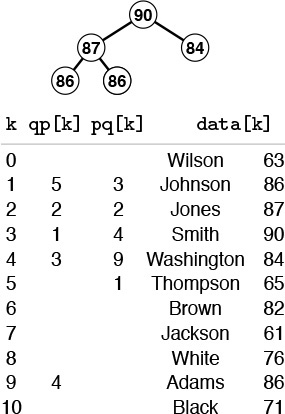
By manipulating indices, rather than the records themselves, we can build a priority queue on a subset of the records in an array. Here, a heap of size 5 in the array pq contains the indices to those students with the top five grades. Thus, data[pq[1]].name contains Smith, the name of the student with the highest grade, and so forth. An inverse array qp allows the priority-queue routines to treat the array indices as handles. For example, if we need to change Smith’s grade to 85, we change the entry in data[3].grade, then call change(3). The priority-queue implementation accesses the record at pq[qp[3]] (or pq[1], because qp[3]=1) and the new key at data[pq[1]].name (or data[3].name, because pq[1]=3).
Figure 9.13 Index heap data structures
Using indices into an existing array is a natural arrangement, but it leads to implementations with an orientation opposite to that of Program 9.8. Now it is the client program that cannot move around information freely, because the priority-queue routine is maintaining indices into data maintained by the client. For its part, the priority queue implementation must not use indices without first being given them by the client.
To develop an implementation, we use precisely the same approach as we did for index sorting in Section 6.8. We manipulate indices and redefine less such that comparisons reference the client’s array. There are added complications here, because it is necessary for the priority-queue routine to keep track of the objects, so that it can find them when the client program refers to them by the handle (array index). To this end, we add a second index array to keep track of the position of the keys in the priority queue. To localize the maintenance of this array, we move data only with the exch operation, then define exch appropriately.
A full implementation of this approach using heaps is given in Program 9.12. This program differs only slightly from Program 9.5, but it is well worth studying because it is so useful in practical situations. We refer to the data structure built by this program as an index heap. We shall use this program as a building block for other algorithms in Parts 5 through 7. As usual, we do no error checking, and we assume (for example) that indices are always in the proper range and that the user does not try to insert anything on a full queue or to remove anything from an empty one. Adding code for such checks is straightforward.
We can use the same approach for any priority queue that uses an array representation (for example, see Exercises 9.50 and 9.51). The main disadvantage of using indirection in this way is the extra space used. The size of the index arrays has to be the size of the data array, when the maximum size of the priority queue could be much less. Another approach to building a priority queue on top of existing data in an array is to have the client program make records consisting of a key with its array index as associated information, or to use an index key with a client-supplied less function. Then, if the implementation uses a linked-allocation representation such as the one in Programs 9.9 and 9.10 or Exercise 9.43, then the space used by the priority queue would be proportional to the maximum number of elements on the queue at any one time. Such approaches would be preferred over Program 9.12 if space must be conserved and if the priority queue involves only a small fraction of the data array.
Contrasting this approach to providing a complete priority-queue implementation to the approach in Section 9.5 exposes essential differences in abstract-data-type design. In the first case (Program 9.8, for example), it is the responsibility of the priority queue implementation to allocate and deallocate the memory for the keys, to change key values, and so forth. The ADT supplies the clent with handles to items, and the client accesses items only through calls to the priority-queue routines, using the handles as arguments. In the second case, (Program 9.12, for example), the client program is responsible for the keys and records, and the priority-queue routines access this information only through handles provided by the user (array indices, in the case of Program 9.12). Both uses require cooperation between client and implementation.
Note that, in this book, we are normally interested in cooperation beyond that encouraged by programming language support mechanisms. In particular, we want the performance characteristics of the implementation to match the dynamic mix of operations required by the client. One way to ensure that match is to seek implementations with provable worst-case performance bounds, but we can solve many problems more easily by matching their performance requirements with simpler implementations.
Exercises
9.48 Suppose that an array is filled with the keys E A S Y Q U E S T I O N. Give the contents of the pq and qp arrays after these keys are inserted into an initially empty heap using Program 9.12.
![]() 9.49 Add a delete operation to Program 9.12.
9.49 Add a delete operation to Program 9.12.
9.50 Implement the priority-queue ADT for index items (see Program 9.11) using an ordered-array representation for the priority queue.
9.51 Implement the priority-queue ADT for index items (see Program 9.11) using an unordered-array representation for the priority queue.
![]() 9.52 Given an array
9.52 Given an array a of N elements, consider a complete binary tree of 2N elements (represented as an array pq) containing indices from the array with the following properties: (i) for i from 0 to N-1, we have pq[N+i]=i; and (ii) for i from 1 to N-1, we have pq[i]=pq[2*i] if a[pq[2*i]]>a[pq[2*i+1]], and we have pq[i]=pq[2*i+1] otherwise. Such a structure is called an index heap tournament because it combines the features of index heaps and tournaments (see Program 5.19). Give the index heap tournament corresponding to the keys E A S Y Q U E S T I O N.
![]() 9.53 Implement the priority-queue ADT for index items (see Program 9.11) using an index heap tournament (see Exercise 9.45).
9.53 Implement the priority-queue ADT for index items (see Program 9.11) using an index heap tournament (see Exercise 9.45).

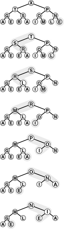
The top diagram depicts a heap that is known to be heap ordered, except possibly at one given node. If the node is larger than its parent, then it must move up, just as depicted in Figure 9.3. This situation is illustrated in the middle diagram, with Y moving up the tree (in general, it might stop before hitting the root). If the node is smaller than the larger of its two children, then it must move down, just as depicted in Figure 9.3. This situation is illustrated in the bottom diagram, with B moving down the tree (in general, it might stop before hitting the bottom). We can use this procedure as the basis for the change priority operation on heaps, to reestablish the heap condition after changing the key in a node; or as the basis for the delete operation on heaps, to reestablish the heap condition after replacing the key in a node with the rightmost key on the bottom level.
Figure 9.14 Changing of the priority of a node in a heap
9.7 Binomial Queues
None of the implementations that we have considered admit implementations of join, delete the maximum, and insert that are all efficient in the worst case. Unordered linked lists have fast join and insert, but slow delete the maximum; ordered linked lists have fast delete the maximum, but slow join and insert; heaps have fast insert and delete the maximum, but slow join; and so forth. (See Table 9.1.) In applications where frequent or large join operations play an important role, we need to consider more advanced data structures.
In this context, we mean by “efficient” that the operations should use no more than logarithmic time in the worst case. This restriction would seem to rule out array representations, because we can join two large arrays apparently only by moving all the elements in at least one of them. The unordered doubly linked-list representation of Program 9.9 does the join in constant time, but requires that we walk through the whole list for delete the maximum. Use of a doubly linked ordered list (see Exercise 9.41) gives a constant-time delete the maximum, but requires linear time to merge lists for join.
Numerous data structures have been developed that can support efficient implementations of all the priority-queue operations. Most of them are based on direct linked representation of heap-ordered trees. Two links are needed for moving down the tree (either to both children in a binary tree or to the first child and next sibling in a binary tree representation of a general tree) and one link to the parent is needed for moving up the tree. Developing implementations of the heap-ordering operations that work for any (heap-ordered) tree shape with explicit nodes and links or other representation is generally straightforward. The difficulty lies in dynamic operations such as insert, delete, and join, which require us to modify the tree structure. Different data structures are based on different strategies for modifying the tree structure while still maintaining balance in the tree. Generally, the algorithms use trees that are more flexible than are complete trees, but keep the trees sufficiently balanced to ensure a logarithmic time bound.
The overhead of maintaining a triply linked structure can be burdensome—ensuring that a particular implementation correctly maintains three pointers in all circumstances can be a significant challenge (see Exercise 9.42). Moreover, in many practical situations, it is difficult to demonstrate that efficient implementations of all the operations are required, so we might pause before taking on such an implementation. On the other hand, it is also difficult to demonstrate that efficient implementations are not required, and the investment to guarantee that all the priority-queue operations will be fast may be justified. Regardless of such considerations, the next step from heaps to a data structure that allows for efficient implementation of join, insert, and delete the maximum is fascinating and worthy of study in its own right.
Even with a linked representation for the trees, the heap condition and the condition that the heap-ordered binary tree be complete are too strong to allow efficient implementation of the join operation. Given two heap-ordered trees, how do we merge them together into just one tree? For example, if one of the trees has 1023 nodes and the other has 255 nodes, how can we merge them into a tree with 1278 nodes, without touching more than 10 or 20 nodes? It seems impossible to merge heap-ordered trees in general if the trees are to be heap ordered and complete, but various advanced data structures have been devised that weaken the heap-order and balance conditions to get the flexibility that we need to devise an efficient join. Next, we consider an ingenious solution to this problem, called the binomial queue, that was developed by Vuillemin in 1978.
To begin, we note that the join operation is trivial for one particular type of tree with a relaxed heap-ordering restriction.
Definition 9.4 A binary tree comprising nodes with keys is said to be left heap ordered if the key in each node is larger than or equal to all the keys in that node’s left subtree (if any).
Definition 9.5 A power-of-2 heap is a left-heap-ordered tree consisting of a root node with an empty right subtree and a complete left subtree. The tree corresponding to a power-of-2 heap by the left-child, right-sibling correspondence is called a binomial tree.
Binomial trees and power-of-2 heaps are equivalent. We work with both representations because binomial trees are slightly easier to visualize, whereas the simple representation of power-of-2 heaps leads to simpler implementations. In particular, we depend upon the following facts, which are direct consequences of the definitions.
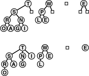
A binomial queue of size N is a list of left-heap-ordered power-of-2 heaps, one for each bit in the binary representation of N. Thus, a binomial queue of size 13 = 11012 consists of an 8-heap, a 4-heap, and a 1-heap. Shown here are the left-heap-ordered power-of-2 heap representation (top) and the heap-ordered binomial-tree representation (bottom) of the same binomial queue.
Figure 9.15 A binomial queue of size 13
• The number of nodes in a power-of-2 heap is a power of 2.
• No node has a key larger than the key at the root.
• Binomial trees are heap-ordered.
The trivial operation upon which binomial queue algorithms are based is that of joining two power-of-2 heaps that have an equal number of nodes. The result is a heap with twice as many nodes that is easy to create, as illustrated in Figure 9.16. The root node with the larger key becomes the root of the result (with the other original root as the result root’s left child), with its left subtree becoming the right subtree of the other root node. Given a linked representation for the trees, the join is a constant-time operation: We simply adjust two links at the top. An implementation is given in Program 9.13. This basic operation is at the heart of Vuillemin’s general solution to the problem of implementing priority queues with no slow operations.
We join two power-of-two heaps (top) by putting the larger of the roots at the root, with that root’s (left) subtree as the right subtree of the other original root. If the operands have 2n nodes, the result has 2n + 1 nodes. If the operands are left-heap ordered, then so is the result, with the largest key at the root. The heap-ordered binomial-tree representation of the same operation is shown below the line.
Figure 9.16 Joining of two equal-sized power-of-2 heaps.
Definition 9.6 A binomial queue is a set of power-of-2 heaps, no two of the same size. The structure of a binomial queue is determined by that queue’s number of nodes, by correspondence with the binary representation of integers.
In accordance with Definitions 9.5 and 9.6, we represent power-of-2 heaps (and handles to items) as links to nodes containing keys and two links (like the explicit tree representation of tournaments in Figure 5.10); and we represent binomial queues as arrays of power-of-2 heaps, as follows:
struct PQnode { Item key; PQlink l, r; };
struct pq { PQlink *bq; };
The arrays are not large and the trees are not high, and this representation is sufficiently flexible to allow implementation of all the priority-queue operations in less than lg N steps, as we shall now see.
A binomial queue of N elements has one power-of-2 heap for each 1 bit in the binary representation of N. For example, a binomial queue of 13 nodes comprises an 8-heap, a 4-heap, and a 1-heap, as illustrated in Figure 9.15. There are at most lg N power-of-2 heaps in a binomial queue of size N, all of height no greater than lg N.
To begin, let us consider the insert operation. The process of inserting a new item into a binomial queue mirrors precisely the process of incrementing a binary number. To increment a binary number, we move from right to left, changing 1s to 0s because of the carry associated with 1 + 1 = 102, until finding the rightmost 0, which we change to 1. In the analogous way, to add a new item to a binomial queue, we move from right to left, merging heaps corresponding to 1 bits with a carry heap, until finding the rightmost empty position to put the carry heap.
Specifically, to insert a new item into a binomial queue, we make the new item into a 1-heap. Then, if N is even (rightmost bit 0), we just put this 1-heap in the empty rightmost position of the binomial queue. If N is odd (rightmost bit 1), we join the 1-heap corresponding to the new item with the 1-heap in the rightmost position of the binomial queue to make a carry 2-heap. If the position corresponding to 2 in the binomial queue is empty, we put the carry heap there; otherwise, we merge the carry 2-heap with the 2-heap from the binomial queue to make a carry 4-heap, and so forth, continuing until we get to an empty position in the binomial queue. This process is depicted in Figure 9.17; Program 9.14 is an implementation.
Adding an element to a binomial queue of seven nodes is analogous to performing the binary addition 1112 + 1 = 10002, with carries at each bit. The result is the binomial queue at the bottom, with an 8-heap and null 4-, 2-, and 1-heaps.
Figure 9.17 Insertion of a new element into a binomial queue
Other binomial-queue operations are also best understood by analogy with binary arithmetic. As we shall see, implementing join corresponds to implementing addition for binary numbers.
For the moment, assume that we have an (efficient) function for join that is organized to merge the priority-queue reference in its second operand with the priority-queue reference in its first operand (leaving the result in the first operand). Using this function, we could implement the insert operation with a call to the join function where one of the operands is a binomial queue of size 1 (see Exercise 9.63).
We can also implement the delete the maximum operation with one call to join. To find the maximum item in a binomial queue, we scan the queue’s power-of-2 heaps. Each of these heaps is left heap-ordered, so it has its maximum element at the root. The largest of the items in the roots is the largest element in the binomial queue. Because there are no more than lg N heaps in the binomial queue, the total time to find the maximum element is less than lg N.
To perform the delete the maximum operation, we note that removing the root of a left-ordered 2k-heap leaves k left-ordered power-of-2 heaps—a 2k–1-heap, a 2k–2-heap, and so forth—which we can easily restructure into a binomial queue of size 2k – 1, as illustrated in Figure 9.18. Then, we can use the join operation to combine this binomial queue with the rest of the original queue, to complete the delete the maximum operation. This implementation is given in Program 9.15.
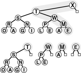
Taking away the root gives a forest of power-of-2 heaps, all left-heap ordered, with roots from the right spine of the tree. This operation leads to a way to delete the maximum element from a binomial queue: Take away the root of the power-of-2 heap that contains the largest element, then use the join operation to merge the resulting binomial queue with remaining power-of-2 heaps in the original binomial queue.
Figure 9.18 Deletion of the maximum in a power-of-2 heap
How do we join two binomial queues? First, we note that the operation is trivial if they do not contain two power-of-2 heaps of the same size, as illustrated in Figure 9.19: we simply merge the heaps from the two binomial queues to make one binomial queue. A queue of size 10 (consisting of an 8-heap and a 2-heap) and a queue of size 5 (consisting of a 4-heap and a 1-heap) simply merge together to make a queue of size 15 (consisting of an 8-heap, a 4-heap, a 2-heap, and a 1-heap). The more general case follows by direct analogy with performing addition on two binary numbers, complete with carry, as illustrated in Figure 9.20.
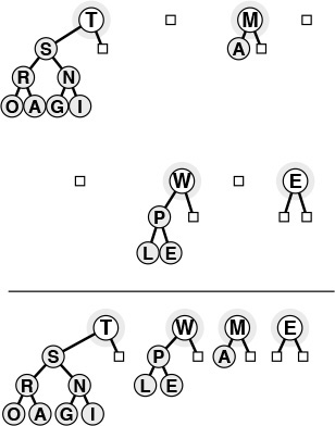
When two binomial queues to be joined do not have any power-of-2 heaps of the same size, the join operation is a simple merge. Doing this operation is analogous to adding two binary numbers without ever encountering 1 + 1 (no carry). Here, a binomial queue of 10 nodes is merged with one of 5 nodes to make one of 15 nodes, corresponding to 10102 + 01012 = 11112.
Figure 9.19 Joining of two binomial queues (no carry)
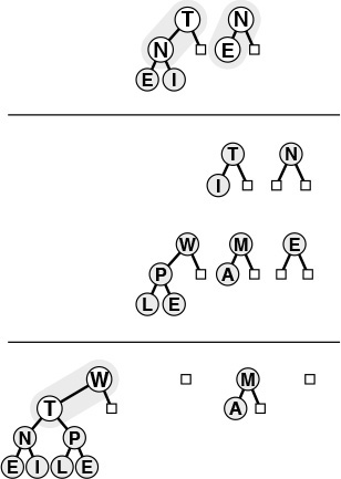
Adding a binomial queue of 3 nodes to one of 7 nodes gives one of 10 nodes through a process that mimics the binary addition 0112 + 1112 = 10102. Adding N to E gives an empty 1-heap in the result with a carry 2-heap containing N and E. Then adding the three 2-heaps leaves a 2-heap in the result with a carry 4-heap containing T N E I. This 4-heap is added to the other 4-heap, producing the binomial queue at the bottom. Few nodes are touched in the process.
Figure 9.20 Joining of two binomial queues
For example, when we add a queue of size 7 (consisting of a 4-heap, a 2-heap, and a 1-heap) to a queue of size 3 (consisting of a 2-heap and a 1-heap), we get a queue of size 10 (consisting of an 8-heap and a 2-heap); to do the addition, we need to merge the 1-heaps and carry a 2-heap, then merge the 2-heaps and carry a 4-heap, then merge the 4-heaps to get an 8-heap result, in a manner precisely analogous to the binary addition 0112 + 1112 = 10102. The example of Figure 9.19 is simpler than Figure 9.20 because it is analogous to 10102 + 01012 = 11112, with no carry.
This direct analogy with binary arithmetic carries through to give us a natural implementation for the join operation (see Program 9.16). For each bit, there are eight cases to consider, based on all the possible different values for the 3 bits involved (carry and two bits in the operands). The code is more complicated than that for plain addition, because we are dealing with distinguishable heaps, rather than with indistinguishable bits, but each case is straightforward. For example, if all 3 bits are 1, we need to leave a heap in the result binomial queue, and to join the other two heaps for the carry into the next position. Indeed, this operation brings us full cycle on abstract data types: we (barely) resist the temptation to cast Program 9.16 as a purely abstract binary addition procedure, with the binomial queue implementation nothing more than a client program using the more complicated bit addition procedure in Program 9.13.
Property 9.7 All the operations for the priority-queue ADT can be implemented with binomial queues such that O(lg N) steps are required for any operations performed on an N-item queue.
These performance bounds are the goal of the design of the data structure. They are direct consequences of the fact that the implementations all have only one or two loops that iterate through the roots of the trees in the binomial queue. For simplicity, our implementations loop through all the trees, so their running time is proportional to the logarithm of the maximum size of the binomial queue. We can make them meet the stated bound for the case when not many items are in the queue by keeping track of the size of the queue, or by using a sentinel pointer value to mark the point where the loops should terminate (see Exercises 9.61 and 9.62). This change may not be worth the effort in many situations, since the maximum queue size is exponentially larger than the maximum number of times that the loop iterates. For example, if we set the maximum size to be 216 and the queue normally has thousands of items, then our simpler implementations iterate the loop 15 times, whereas the more complicated methods still need to iterate perhaps 11 or 12 times, and they incur extra cost for maintaining the size or the sentinel. On the other hand, blindly setting a large maximum might cause our programs to run more slowly than expected for tiny queues. ![]()
Property 9.8 Construction of a binomial queue with N insert operations on an initially empty queue requires O(N) comparisons in the worst case.
For one-half the insertions (when the queue size is even and there is no 1-heap) no comparisons are required; for one-half the remaining insertions (when there is no 2-heap) only 1 comparison is required; when there is no 4-heap, only 2 comparisons are required; and so forth. Thus, the total number of comparisons is less than 0 · N/2 + 1 · N/4 + 2 · N/8 + ... < N. As for Property 9.7, we also need one of the modifications discussed in Exercises 9.61 and 9.62 to get the stated linear worst-case time bound. ![]()
As discussed in Section 4.8, we have not considered memory allocation in the implementation of join in Program 9.16, so it has a memory leak, and therefore may be unusable in some situations. To correct this defect, we need to pay proper attention to memory allocation for the arguments and return value of the function that implements join (see Exercise 9.65).
Binomial queues provide guaranteed fast performance, but data structures have been designed with even better theoretical performance characteristics, providing guaranteed constant-time performance for certain operations. This problem is an interesting and active area of data-structure design. On the other hand, the practical utility of many of these esoteric structures is dubious, and we need to be certain that performance bottlenecks exist that we can relieve only by reducing the running time of some priority-queue operation, before we delve into complex data-structure solutions. Indeed, for practical applications, we should prefer a trivial structure for debugging and for small queues; then, we should use heaps to speed up the operations unless fast join operations are required; finally, we should use binomial queues to guarantee logarithmic performance for all operations. All things considered, however, a priority-queue package based on binomial queues is a valuable addition to a software library.
![]() 9.55 Write a program to draw the binomial-tree representation of a binomial queue, given the size N (just nodes connected by edges, no keys).
9.55 Write a program to draw the binomial-tree representation of a binomial queue, given the size N (just nodes connected by edges, no keys).
9.56 Give the binomial queue that results when the keys E A S Y Q U E S T I O N are inserted into an initially empty binomial queue.
9.57 Give the binomial queue that results when the keys E A S Y are inserted into an initially empty binomial queue, and give the binomial queue that results when the keys Q U E S T I O N are inserted into an initially empty binomial queue. Then give the result of delete the maximum for each queue. Finally, give the result when the join operation is performed on the resulting queues.
9.58 Using the conventions of Exercise 9.1 give the sequence of binomial queues produced when the operations
P R I O * R * * I * T * Y * * * Q U E * * * U * E
are performed on an initially empty binomial queue.
9.59 Using the conventions of Exercise 9.2 give the sequence of binomial queues produced when the operations
( ( ( P R I O *) + ( R * I T * Y * ) ) * * * ) + ( Q U E * * * U * E )
are performed on an initially empty binomial queue.
9.60 Prove that a binomial tree with 2n nodes has ![]() nodes at level i for 0 ≤ i ≤ n. (This fact is the origin of the name binomial tree.)
nodes at level i for 0 ≤ i ≤ n. (This fact is the origin of the name binomial tree.)
![]() 9.61 Implement binomial queues such that Property 9.7 holds, by modifying the binomial-queue data type to include the queue size, then using the size to control the loops.
9.61 Implement binomial queues such that Property 9.7 holds, by modifying the binomial-queue data type to include the queue size, then using the size to control the loops.
![]() 9.62 Implement binomial queues such that Property 9.7 holds, by maintaining a sentinel pointer to mark the point where the loops should terminate.
9.62 Implement binomial queues such that Property 9.7 holds, by maintaining a sentinel pointer to mark the point where the loops should terminate.
![]() 9.63 Implement insert for binomial queues by just using the join operation explicitly.
9.63 Implement insert for binomial queues by just using the join operation explicitly.
![]() 9.64 Implement change priority and delete for binomial queues. Note: You will need to add a third link, which points up the tree, to the nodes.
9.64 Implement change priority and delete for binomial queues. Note: You will need to add a third link, which points up the tree, to the nodes.
![]() 9.65 Modify the priority queue ADT interface (Program 9.8) and binomial queue implementations (Programs 9.13 through 9.16) in the text such that there are no memory leaks (see Exercise 4.72).
9.65 Modify the priority queue ADT interface (Program 9.8) and binomial queue implementations (Programs 9.13 through 9.16) in the text such that there are no memory leaks (see Exercise 4.72).
![]() 9.66 Empirically compare binomial queues against heaps as the basis for sorting, as in Program 9.6, for randomly ordered keys with N = 1000, 104, 105, and 106. Note: See Exercises 9.61 and 9.62.
9.66 Empirically compare binomial queues against heaps as the basis for sorting, as in Program 9.6, for randomly ordered keys with N = 1000, 104, 105, and 106. Note: See Exercises 9.61 and 9.62.
![]() 9.67 Develop an in-place sorting method like heapsort, but based on binomial queues. Hint: See Exercise 9.37.
9.67 Develop an in-place sorting method like heapsort, but based on binomial queues. Hint: See Exercise 9.37.