Chapter Twelve. Symbol Tables and Binary Search Trees
The retrieval of a particular piece or pieces of information from large volumes of previously stored data is a fundamental operation, called search, that is intrinsic to a great many computational tasks. As with sorting algorithms in Chapters 6 through 11, and in particular priority queues in Chapter 9, we work with data divided into records or items, each item having a key for use in searching. The goal of the search is to find the items with keys matching a given search key. The purpose of the search is usually to access information within the item (not merely the key) for processing.
Applications of search are widespread, and involve a variety of different operations. For example, consider a bank that needs to keep track of all its customers’ account information and to search through these records to check account balances and to perform transactions. Another example is an airline that needs to keep track of reservations on all its flights, and to search through them to find empty seats or to cancel or otherwise modify the reservations. A third example is a search engine on a network software interface that looks for all documents in the network containing a given keyword. The demands of these applications are similar in some ways (the bank and the airline both demand accuracy and reliability) and different in others (the bank’s data have a long life, compared to the data in the others); all need good search algorithms.
Definition 12.1 A symbol table is a data structure of items with keys that supports two basic operations: insert a new item, and return an item with a given key.
Symbol tables are also sometimes called dictionaries, by analogy with the time-honored system of providing definitions for words by listing them alphabetically in a reference book. In an English-language dictionary, the “keys” are the words and the “items” are the entries associated with the words that contain the definition, pronunciation, and other information. People use search algorithms to find information in a dictionary, usually depending on the fact that the entries appear in alphabetical order. Telephone books, encyclopedias, and other reference books are organized in essentially the same way, and some of the search methods that we shall discuss (for example the binary search algorithm in Sections 2.6 and 12.4) also depend upon the entries being kept in order.
An advantage of computer-based symbol tables is that they can be much more dynamic than a dictionary or a telephone book, so most of the methods that we shall discuss build data structures that not only enable efficient search algorithms, but also support efficient implementations of operations to add new items, to delete or modify items, to combine two symbol tables into one, and so forth. In this chapter, we shall revisit many of the issues related to such operations that we considered for priority queues in Chapter 9. The development of dynamic data structures to support search is one of the oldest and most widely studied problems in computer science; it will be our main focus in this chapter and in Chapters 13 through 16. As we shall see, many ingenious algorithms have been (and are still being) invented to solve the symbol-table implementation problem.
Beyond basic applications of the type just mentioned, symbol tables have been studied intensively by computer scientists and programmers because they are indispensable aids in organizing software on computer systems. A symbol table is the dictionary for a program: The keys are the symbolic names used in the program, and the items contain information describing the object named. From the early days of computing, when symbol tables allowed programmers to move from using numeric addresses in machine code to using symbolic names in assembly language, to modern applications of the new millennium, when symbolic names have meaning across worldwide computer networks, fast search algorithms have played and will play an essential role in computation.
Symbol tables are also frequently encountered in low-level abstractions, occasionally at the hardware level. The term associative memory is sometimes used to describe the concept. We shall focus on software implementations, but some of the methods that we consider are also appropriate for hardware implementation.
As with our study of sorting methods in Chapter 6, we shall begin our study of search methods in this chapter by looking at some elementary methods that are useful for small tables and in other special situations and that illustrate fundamental techniques exploited by more advanced methods. Then, for much of the remainder of the chapter, we shall focus on the binary search tree (BST), a fundamental and widely used data structure that admits fast search algorithms.
We considered two search algorithms in Section 2.6 as an illustration of the effectiveness of mathematical analysis in helping us to develop effective algorithms. For completeness in this chapter, we repeat some of the information that we considered in Section 2.6, though we refer back to that section for some proofs. Later in the chapter, we also refer to the basic properties of binary trees that we considered in Sections 5.4 and 5.5.
12.1 Symbol-Table Abstract Data Type
As with priority queues, we think of search algorithms as belonging to interfaces declaring a variety of generic operations that can be separated from particular implementations, so that we can easily substitute alternate implementations. The operations of interest include
• Insert a new item.
• Search for an item (or items) having a given key.
• Delete a specified item.
• Select the kth smallest item in a symbol table.
• Sort the symbol table (visit all the items in order of their keys).
• Join two symbol tables.
As we do with many data structures, we might also need to add standard initialize, test if empty, and perhaps destroy and copy operations to this set. In addition, we might wish to consider various other practical modifications of the basic interface. For example, a search-and-insert operation is often attractive because, for many implementations, the search for a key, even if unsuccessful, nevertheless gives precisely the information needed to insert a new item with that key.
We commonly use the term “search algorithm” to mean “symbol-table ADT implementation,” although the latter more properly implies defining and building an underlying data structure for the symbol table and implementing ADT operations in addition to search. Symbol tables are so important to so many computer applications that they are available as high-level abstractions in many programming environments (the C standard library has bsearch, an implementation of the binary search algorithm in Section 12.4). As usual, it is difficult for a general-purpose implementation to meet the demanding performance needs of diverse applications. Our study of many of the ingenious methods that have been developed to implement the symbol-table abstraction will set a context to help us decide when to use a prepackaged implementation and when to develop one that is tailored to a particular application.
As we did with sorting, we will consider the methods without specifying the types of the items being processed. In the same manner that we discussed in detail in Section 6.8, we consider implementations that use an interface that defines Item and the basic abstract operations on the data. We consider both comparison-based methods and radix-based methods that use keys or pieces of keys as indices. To emphasize the separate roles played by items and keys in search, we extend the Item concept that we used in Chapters 6 through 11 such that items contain keys of type Key. For the simple cases that we commonly use when describing algorithms where items consist solely of keys, Key and Item are the same, and this change has no effect, but adding the Key type allows us to be clear about when we are referring to items and when we are referring to keys. We also use a macro key for storing keys in or extracting them from items and use the basic operation eq for testing whether two keys are equal. In this chapter and in Chapter 13, we also use the operation less for comparing two key values, to guide us in the search; in Chapters 14 and 15, our search algorithms are based on extracting pieces of keys using the basic radix operations that we used in Chapter 10. We use the constant NULLitem as a return value when no item in the symbol table has the search key. To use the interfaces and implementations for floating-point numbers, strings, and more complicated items from Sections 6.8 and 6.9 for search, we need only to implement appropriate definitions for Key, key, NULLitem, eq, and less.
Program 12.1 is an interface that defines the basic symbol-table operations (except join). We shall use this interface between client programs and all the search implementations in this and the next several chapters. We could also define a version of the interface in Program 12.1 to have each function take a symbol-table handle as an argument, in a manner similar to Program 9.8, to implement first-class symbol-table ADTs that provide clients with the capability to use multiple symbol tables (containing objects of the same type) (see Section 4.8), but this arrangement unnecessarily complicates programs that use only one table (see Exercise 12.4). We also can define a version of the interface in Program 12.1 to manipulate handles to items in a manner similar to Program 9.8 (see Exercise 12.5), but this arrangement unnecessarily complicates the programs in the typical situation where it suffices to manipulate an item by the key. By assuming, in our implementations, that only one symbol table is in use, maintained by the ADT, we are able to focus on the algorithms without being distracted by packaging considerations. We shall return to this issue occasionally, when appropriate. In particular, when discussing algorithms for delete, we need to be aware that implementations that provide handles obviate the need to search before deleting, and so can admit faster algorithms for some implementations. Also, the join operation is defined only for first-class symbol-table ADT implementations, so we need a first-class ADT when we consider algorithms for join (see Section 12.9).
Some algorithms do not assume any implied ordering among the keys and therefore use only eq (and not less) to compare keys, but many of the symbol-table implementations use the ordering relationship among keys implied by less to structure the data and to guide the search. Also, the select and sort abstract operations explicitly refer to key order. The sort function is packaged as a function that processes all the items in order, without necessarily rearranging them. This setup makes it easy, for example, to print them out in sorted order while still maintaining the flexibility and efficiency of the dynamic symbol table. Algorithms that do not use less do not require that keys be comparable to one another, and do not necessarily support select and sort.
The possibility of items with duplicate keys should receive special consideration in a symbol-table implementation. Some applications disallow duplicate keys, so keys can be used as handles. An example of this situation is the use of social-security numbers as keys in personnel files. Other applications may involve numerous items with duplicate keys: for example, keyword search in document databases typically will result in multiple search hits.
We can handle items with duplicate keys in one of several ways. One approach is to insist that the primary search data structure contain only items with distinct keys, and to maintain, for each key, a link to a list of application items with duplicate keys. That is, we use items that contain a key and a link in our primary data structures, and do not have items with duplicate keys. This arrangement is convenient in some applications, since all the items with a given search key are returned with one search or can be removed with one delete. From the point of view of the implementation, this arrangement is equivalent to leaving duplicate-key management to the client. A second possibility is to leave items with equal keys in the primary search data structure, and to return any item with the given key for a search. This convention is simpler for applications that process one item at a time, where the order in which items with duplicate keys are processed is not important. It may be inconvenient in terms of the algorithm design, because the interface might have to be extended to include a mechanism to retrieve all items with a given key or to call a specified function for each item with the given key. A third possibility is to assume that each item has a unique identifier (apart from the key), and to require that a search find the item with a given identifier, given the key. Or some more complicated mechanism might be necessary. These considerations apply to all the symbol-table operations in the presence of duplicate keys. Do we want to delete all items with the given key, or any item with the key, or a specific item (which requires an implementation that provides handles to items)? When describing symbol table implementations, we indicate informally how items with duplicate keys might be handled most conveniently, without necessarily considering each mechanism for each implementation.
Program 12.2 is a sample client program that illustrates these conventions for symbol-table implementations. It uses a symbol table to find the distinct values in a sequence of keys (randomly generated or read from standard input), then prints them out in sorted order.
As usual, we have to be aware that differing implementations of the symbol-table operations have differing performance characteristics, which may depend on the mix of operations. One application might use insert relatively infrequently (perhaps to build a table), then follow up with a huge number of search operations; another application might use insert and delete a huge number of times on relatively small tables, intermixed with search operations. Not all implementations will support all operations, and some implementations might provide efficient support of certain functions at the expense of others, with an implicit assumption that the expensive functions are performed rarely. Each of the fundamental operations in the symbol table interface has important applications, and many basic organizations have been suggested to support efficient use of various combinations of the operations. In this and the next few chapters, we shall concentrate on implementations of the fundamental functions initialize, insert, and search, with some comment on delete, select, sort, and join when appropriate. The wide variety of algorithms to consider stems from differing performance characteristics for various combinations of the basic operations, and perhaps also from constraints on key values, or item size, or other considerations.
In this chapter, we shall see implementations where search, insert, delete, and select take time proportional to the logarithm of the number of items in the dictionary, on the average, for random keys, and sort runs in linear time. In Chapter 13, we shall examine ways to guarantee this level of performance, and we shall see one implementation in Section 12.2 and several in Chapters 14 and 15 with constant-time performance under certain circumstances.
Many other operations on symbol tables have been studied. Examples include finger search, where a search can begin from the point where a previous search ended; range search, where we want to count or visit all the nodes falling within a specified interval; and, when we have a concept of distance between keys, near-neighbor search, where we want to find items with keys closest to a given key. We consider such operations in the context of geometric algorithms, in Part 6.
Exercises
![]() 12.1 Use the symbol-table ADT Program 12.1 to implement stack and queue ADTs.
12.1 Use the symbol-table ADT Program 12.1 to implement stack and queue ADTs.
![]() 12.2 Use the symbol-table ADT defined by the interface Program 12.1 to implement a priority-queue ADT that supports both delete-the-maximum and delete-the-minimum operations.
12.2 Use the symbol-table ADT defined by the interface Program 12.1 to implement a priority-queue ADT that supports both delete-the-maximum and delete-the-minimum operations.
12.3 Use the symbol-table ADT defined by the interface Program 12.1 to implement an array sort compatible with those in Chapters 6 through 10.
12.4 Define an interface for a first-class symbol-table ADT, which allows client programs to maintain multiple symbol tables and to combine tables (see Sections 4.8 and 9.5).
12.5 Define an interface for a symbol-table ADT that allows client programs to delete specific items via handles and to change keys (see Sections 4.8 and 9.5).
![]() 12.6 Give an item-type interface and implementation for items with two fields: a 16-bit integer key and a string that contains information associated with the key.
12.6 Give an item-type interface and implementation for items with two fields: a 16-bit integer key and a string that contains information associated with the key.
12.7 Give the average number of distinct keys that our example driver program (Program 12.2) will find among N random positive integers less than 1000, for N = 10, 102, 103, 104, and 105. Determine your answer empirically, or analytically, or both.
12.2 Key-Indexed Search
Suppose that the key values are distinct small numbers. In this case, the simplest search algorithm is based on storing the items in an array, indexed by the keys, as in the implementation given in Program 12.3. The code is straightforward: We initialize all the entries with NULLitem, then insert an item with key value k simply by storing it in st[k], and search for an item with key value k by looking in st[k]. To delete an item with key value k, we put NULLitem in st[k]. The select, sort, and count implementations in Program 12.3 use a linear scan through the array, skipping null items. The implementation leaves to the client the tasks of handling items with duplicate keys and checking for conditions such as specifying delete for a key not in the table.
This implementation is a point of departure for all the symbol-table implementations that we consider in this chapter and in Chapters 13 through 15. With the indicated include directives, it can be compiled separately from any particular client and used as an implementation for numerous different clients, and with different item types. The compiler will check that interface, implementation, and client adhere to the same defined conventions.
The indexing operation upon which key-indexed search is based is the same as the basic operation in the key-indexed counting sort method that we examined in Section 6.10. Key-indexed search is the method of choice, when it is applicable, because search and insert could hardly be implemented more efficiently.
If there are no items at all (just keys), we can use a table of bits. The symbol table in this case is called an existence table, because we may think of the kth bit as signifying whether k exists among the set of keys in the table. For example, we could use this method to determine quickly whether a given 4-digit number in a telephone exchange has already been assigned, using a table of 313 words on a 32-bit computer (see Exercise 12.12).
Property 12.1 If key values are positive integers less than M and items have distinct keys, then the symbol-table data type can be implemented with key-indexed arrays of items such that insert, search, and delete require constant time; and initialize, select, and sort require time proportional to M, whenever any of the operations are performed on an N-item table.
This fact is immediate from inspection of the code. Note that the conditions on the keys imply that N ≤ M. ![]()
Program 12.3 does not handle duplicate keys, and it assumes that the key values are between 0 and maxKey-1. We could use linked lists or one of the other approaches mentioned in Section 12.1 to store any items with duplicate keys, and we could do simple transformations of the keys before using them as indices (see Exercise 12.11), but we defer considering these cases in detail to Chapter 14, when we consider hashing, which uses this same approach to implement symbol tables for general keys, by transforming keys from a potentially large range such that they fall within a small range, then taking appropriate action for items with duplicate keys. For the moment, we assume that an old item with a key value equal to the key in an item to be inserted can be silently ignored (as in Program 12.3), or treated as an error condition (see Exercise 12.8).
The implementation of count in Program 12.3 is a lazy approach where we do work only when the function STcount is called. An alternative (eager) approach is to maintain the count of nonempty table positions in a local variable, incrementing the variable if insert is into a table position that contains NULLitem, and decrementing it if delete is for a table position that does not contain NULLitem (see Exercise 12.9). The lazy approach is the better of the two if the count operation is used rarely (or not at all) and the number of possible key values is small; the eager approach is better if the count operation is used often or the number of possible key values is huge. For a general-purpose library routine, the eager approach is preferred, because it provides optimal worst-case performance at the cost of a small constant factor for insert and delete; for the inner loop in an application with a huge number of insert and delete operations but few count operations, the lazy approach is preferred, because it gives the fastest implementation of the common operations. This type of dilemma is common in the design of ADTs that must support a varying mix of operations, as we have seen on several occasions.
For a full implementation of a first-class symbol-table ADT (see Section 4.8) using a key-indexed array as the underlying data structure, we could allocate the array dynamically, and use its address as a handle. There are various other design decisions that we also need to make in developing such an interface. For example, should the key range be the same for all objects, or be different for different objects? If the latter option is chosen, then it may be necessary to have a function giving the client access to the key range.
Key-indexed arrays are useful for many applications, but they do not apply if keys do not fall into a small range. Indeed, we might think of this and the next several chapters as being concerned with designing solutions for the case where the keys are from such a large range that it is not feasible to have an indexed table with one potential place for each key.
Exercises
12.8 Implement an interface for a first-class symbol-table ADT (see Exercise 12.4), using dynamically allocated key-indexed arrays.
![]() 12.9 Modify the implementation of Program 12.3 to provide an eager implementation of
12.9 Modify the implementation of Program 12.3 to provide an eager implementation of STcount (by keeping track of the number of nonnull entries).
![]() 12.10 Modify your implementation from Exercise 12.8 to provide an eager implementation of
12.10 Modify your implementation from Exercise 12.8 to provide an eager implementation of STcount (see Exercise 12.9).
12.11 Modify the implementation and interface of Program 12.1 and Program 12.3 to use a function h(Key) that converts keys to nonnegative integers less than M, with no two keys mapping to the same integer. (This improvement makes the implementation useful whenever keys are in a small range (not necessarily starting at 0) and in other simple cases.)
12.12 Modify the implementation and interface of Program 12.1 and Program 12.3 for the case when items are keys that are positive integers less than M (no associated information). In the implementation, use a dynamically allocated array of about M/bitsword words, where bitsword is the number of bits per word on your computer system.
12.13 Use your implementation from Exercise 12.12 for experiments to determine empirically the average and standard deviation for the number of distinct integers in a random sequence of N nonnegative integers less than N, for N close to the memory available to a program on your computer, expressed as a number of bits (see Program 12.2).
12.3 Sequential Search
For general key values from too large a range for them to be used as indices, one simple approach for a symbol-table implementation is to store the items contiguously in an array, in order. When a new item is to be inserted, we put it into the array by moving larger elements over one position as we did for insertion sort; when a search is to be performed, we look through the array sequentially. Because the array is in order, we can report a search miss when we encounter a key larger than the search key. Moreover, since the array is in order, both select and sort are trivial to implement. Program 12.4 is a symbol-table implementation that is based on this approach.
We could slightly improve the inner loop in the implementation of search in Program 12.4 by using a sentinel to eliminate the test for running off the end of the array in the case that no item in the table has the search key. Specifically, we could reserve the position after the end of the array as a sentinel, then fill its key field with the search key before a search. Then the search will always terminate with an item containing the search key, and we can determine whether or not the key was in the table by checking whether that item is the sentinel.
Alternatively, we could develop an implementation where we do not insist that the items in the array be kept in order. When a new item is to be inserted, we put it at the end of the array; when a search is to be performed we look through the array sequentially. The characteristic property of this approach is that insert is fast but select and sort require substantially more work (they each require one of the methods in Chapters 7 through 10). We can delete an item with a specified key by doing a search for it, then moving the final item in the array to its position and decrementing the size by 1; and we can delete all items with a specified key by iterating this operation. If a handle giving the index of an item in the array is available, the search is unnecessary and delete takes constant time.
Another straightforward option for a symbol-table implementation is to use a linked list. Again, we can choose to keep the list in order, to be able to easily support the sort operation, or to leave it unordered, so that insert can be fast. Program 12.5 is an implementation of the latter. As usual, the advantage of using linked lists over arrays is that we do not have to predict the maximum size of the table in advance; the disadvantages are that we need extra space (for the links) and we cannot support select efficiently.
The unordered-array and ordered-list approaches are left for exercises (see Exercise 12.18 and Exercise 12.19). These four implementation approaches (array or list, ordered or unordered) could be used interchangeably in applications, differing only (we expect) in time and space requirements. In this and the next several chapters, we will examine numerous different approaches to the symbol-table–implementation problem.
Keeping the items in order is an illustration of the general idea that symbol-table implementations generally use the keys to structure the data in some way to provide for fast search. The structure might allow fast implementations of some of the other operations, but this savings has to be balanced against the cost of maintaining the structure, which might be slowing down other operations. We shall see many examples of this phenomenon. For example, in an application where the sort function is needed frequently, we would choose an ordered (array or list) representation because the chosen structure of the table makes the sort function trivial, as opposed to it needing a full sort implementation. In an application where we know that the select operation might be performed frequently, we would choose an ordered array representation because this structure of the table makes select constant-time. By contrast, select takes linear time in a linked list, even an ordered one.
To analyze the performance of sequential search for random keys in more detail, we begin by considering the cost of inserting new keys and by considering separately the costs of successful and unsuccessful searches. We often refer to the former as a search hit, and to the latter as a search miss. We are interested in the costs for both hits and misses, on the average and in the worst case. Strictly speaking, our ordered-array implementation (see Program 12.4) uses two comparisons for each item examined (one eq and one less). For the purposes of analysis, we regard such a pair as a single comparison throughout Chapters 12 through 16, since we normally can do low-level optimizations to effectively combine them.
Property 12.2 Sequential search in a symbol table with N items uses about N/2 comparisons for search hits (on the average).
See Property 2.1. The argument applies for arrays or linked lists, ordered or unordered. ![]()
Property 12.3 Sequential search in a symbol table of N unordered items uses a constant number of steps for inserts and N comparisons for search misses (always).
These facts are true for both the array and linked-list representations, and are immediate from the implementations (see Exercise 12.18 and Program 12.5). ![]()
Property 12.4 Sequential search in a symbol table of N ordered items uses about N/2 comparisons for insertion, search hits, and search misses (on the average).
See Property 2.2. Again, these facts are true for both the array and linked-list representations, and are immediate from the implementations (see Program 12.4 and Exercise 12.19). ![]()
Building an ordered table by successive insertion is essentially equivalent to running the insertion-sort algorithm of Section 6.2. The total running time to build the table is quadratic, so we would not use this method for large tables. If we have a huge number of search operations in a small table, then keeping the items in order is worthwhile, because Properties 12.3 and 12.4 tell us that this policy can save a factor of 2 in the time for search misses. If items with duplicate keys are not to be kept in the table, the extra cost of keeping the table in order is not as burdensome as it might seem, because an insertion happens only after a search miss, so the time for insertion is proportional to the time for search. On the other hand, if items with duplicate keys may be kept in the table, we can have a constant-time insert implementation with an unordered table. The use of an unordered table is preferred for applications where we have a huge number of insert operations and relatively few search operations.
Beyond these differences, we have the standard tradeoff that linked-list implementations use space for the links, whereas array implementations require that the maximum table size be known ahead of time or that the table undergo amortized growth (see Section 14.5). Also, as discussed in Section 12.9, a linked-list implementation has the flexibility to allow efficient implementation of other operations such as join and delete, in first-class symbol-table ADT implementations.
Table 12.1 summarizes these results, and puts them in context with other search algorithms discussed later in this chapter and in Chapters 13 and 14. In Section 12.4 we consider binary search, which brings the search time down to lg N and is therefore widely used for static tables (when insertions are relatively infrequent).
The entries in this table are running times within a constant factor as a function of N, the number of items in the table, and M, the size of the table (if different from N), for implementations where we can insert new items without regard to whether items with duplicate keys are in the table. Elementary methods (first four lines) require constant time for some operations and linear time for others; more advanced methods yield guaranteed logarithmic or constant-time performance for most or all operations. The N lg N entries in the column for select represent the cost of sorting the items—a linear-time select for an unordered set of items is possible in theory, but is not practical (see Section 7.8). Starred entries indicate worst-case events that are extremely unlikely.
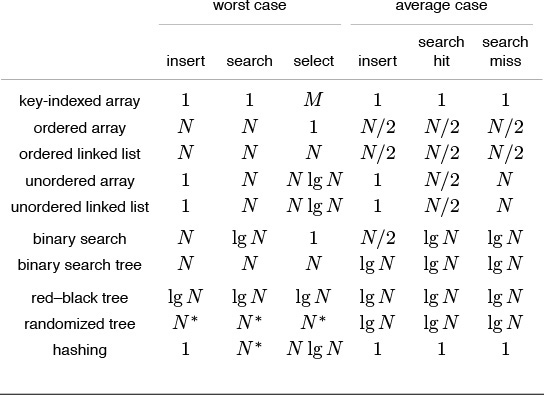
Table 12.1 Costs of insertion and search in symbol tables
In Sections 12.5 through 12.9, we consider binary search trees, which have the flexibility to admit search and insertion in time proportional to lg N, but only on the average. In Chapter 13, we shall consider red-black trees and randomized binary search trees, which guarantee logarithmic performance or make it extremely likely, respectively. In Chapter 14, we shall consider hashing, which provides constant-time search and insertion, on the average, but does not efficiently support sort and some other operations. In Chapter 15, we shall consider the radix search methods that are analogous to the radix sorting methods of Chapter 10; in Chapter 16, we shall consider methods that are appropriate for files that are stored externally.
Exercises
![]() 12.14 Add an implementation for the delete operation to our ordered-array–based symbol-table implementation (Program 12.4).
12.14 Add an implementation for the delete operation to our ordered-array–based symbol-table implementation (Program 12.4).
![]() 12.15 Implement
12.15 Implement STsearchinsert functions for our list-based (Program 12.5) and array-based (Program 12.4) symbol-table implementations. They should search the symbol table for items with the same key as a given item, then insert the item if there is none.
12.16 Implement a select operation for our list-based symbol-table implementation (Program 12.5).
12.17 Give the number of comparisons required to put the keys E A S Y Q U E S T I O N into an initially empty table using ADTs that are implemented with each of the four elementary approaches: ordered or unordered array or list. Assume that a search is performed for each key, then an insertion is done for search misses, as in Exercise 12.15.
12.18 Implement the initialize, search, and insert operations for the symbol-table interface in Program 12.1, using an unordered array to represent the symbol table. Your program should match the performance characteristics set forth in Table 12.1.
![]() 12.19 Implement the initialize, search, insert, and sort operations for the symbol-table interface in Program 12.1, using an ordered linked list to represent the symbol table. Your program should meet the performance characteristics set forth in Table 12.1.
12.19 Implement the initialize, search, insert, and sort operations for the symbol-table interface in Program 12.1, using an ordered linked list to represent the symbol table. Your program should meet the performance characteristics set forth in Table 12.1.
![]() 12.20 Change our list-based symbol-table implementations (Program 12.5) to support a first-class symbol-table ADT with client item handles (see Exercises 12.4 and 12.5), then add delete and join operations.
12.20 Change our list-based symbol-table implementations (Program 12.5) to support a first-class symbol-table ADT with client item handles (see Exercises 12.4 and 12.5), then add delete and join operations.
12.21 Write a performance driver program that uses STinsert to fill a symbol table, then uses STselect and STdelete to empty it, doing so multiple times on random sequences of keys of various lengths ranging from small to large; measures the time taken for each run; and prints out or plots the average running times.
12.22 Write a performance driver program that uses STinsert to fill a symbol table, then uses STsearch such that each item in the table is hit an average of 10 times and there is about the same number of misses, doing so multiple times on random sequences of keys of various lengths ranging from small to large; measures the time taken for each run; and prints out or plots the average running times.
12.23 Write an exercise driver program that uses the functions in our symbol-table interface Program 12.1 on difficult or pathological cases that might turn up in practical applications. Simple examples include files that are already in order, files in reverse order, files where all keys are the same, and files consisting of only two distinct values.
![]() 12.24 Which symbol-table implementation would you use for an application that does 102 insert operations, 103 search operations, and 104 select operations, randomly intermixed? Justify your answer.
12.24 Which symbol-table implementation would you use for an application that does 102 insert operations, 103 search operations, and 104 select operations, randomly intermixed? Justify your answer.
![]() 12.25 (This exercise is five exercises in disguise.) Answer Exercise 12.24 for the other five possibilities of matching up operations and frequency of use.
12.25 (This exercise is five exercises in disguise.) Answer Exercise 12.24 for the other five possibilities of matching up operations and frequency of use.
12.26 A self-organizing search algorithm is one that rearranges items to make those that are accessed frequently likely to be found early in the search. Modify your search implementation for Exercise 12.18 to perform the following action on every search hit: move the item found to the beginning of the list, moving all items between the beginning of the list and the vacated position to the right one position. This procedure is called the move-to-front heuristic.
![]() 12.27 Give the order of the keys after items with the keys E A S Y Q U E S T I O N have been put into an initially empty table with search, then insert on search miss, using the move-to-front self-organizing search heuristic (see Exercise 12.26).
12.27 Give the order of the keys after items with the keys E A S Y Q U E S T I O N have been put into an initially empty table with search, then insert on search miss, using the move-to-front self-organizing search heuristic (see Exercise 12.26).
12.28 Write a driver program for self-organizing search methods that uses STinsert to fill a symbol table with N keys, then does 10N searches to hit items according to a predefined probability distribution.
12.29 Use your solution to Exercise 12.28 to compare the running time of your implementation from Exercise 12.18 with your implementation from Exercise 12.26, for N = 10, 100, and 1000, using the probability distribution where search is for the ith largest key with probability 1/2i for 1 ≤ i ≤ N.
12.30 Do Exercise 12.29 for the probability distribution where search is for the ith largest key with probability HN /i for 1 ≤ i ≤ N. This distribution is called Zipf’s law.
12.31 Compare the move-to-front heuristic with the optimal arrangement for the distributions in Exercises 12.29 and 12.30, which is to keep the keys in increasing order (decreasing order of their expected frequency). That is, use Program 12.4, instead of your solution to Exercise 12.18, in Exercise 12.29.
12.4 Binary Search
In the array implementation of sequential search, we can reduce significantly the total search time for a large set of items by using a search procedure based on applying the standard divide-and-conquer paradigm (see Section 5.2): Divide the set of items into two parts, determine to which of the two parts the search key belongs, then concentrate on that part. A reasonable way to divide the sets of items into parts is to keep the items sorted, then to use indices into the sorted array to delimit the part of the array being worked on. This search technique is called binary search. Program 12.6 is a recursive implementation of this fundamental strategy. Program 2.2 is a nonrecursive implementation of the method—no stack is needed because the recursive function in Program 12.6 ends in a recursive call.
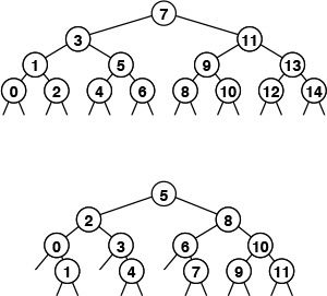
Figure 12.1 shows the subfiles examined by binary search when a small table is searched; Figure 12.2 depicts a larger example. Each iteration eliminates slightly more than one-half of the table, so the number of iterations required is small.
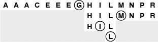
Binary search uses only three iterations to find a search key L in this sample file. On the first call, the algorithm compares L to the key in the middle of the file, the G. Since L is larger, the next iteration involves the right half of the file. Then, since L is less than the M in the middle of the right half, the third iteration involves the subfile of size 3 containing H, I, and L. After one more iteration, the subfile size is 1, and the algorithm finds the L.
Figure 12.1 Binary search
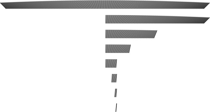
With binary search, we need only seven iterations to find a record in a file of 200 elements. The subfile sizes follow the sequence 200, 99, 49, 24, 11, 5, 2, 1; each is slightly less than one-half of the previous.
Figure 12.2 Binary search
Property 12.5 Binary search never uses more than ![]() lg N
lg N![]() + 1 comparisons for a search (hit or miss).
+ 1 comparisons for a search (hit or miss).
See Property 2.3. It is amusing to note that the maximum number of comparisons used for a binary search in a table of size N is precisely the number of bits in the binary representation of N, because the operation of shifting 1 bit to the right converts the binary representation of N into the binary representation of ![]() N/2
N/2![]() (see Figure 2.6).
(see Figure 2.6). ![]()
Keeping the table sorted as we do in insertion sort leads to a running time that is a quadratic function of the number of insert operations, but this cost might be tolerable or even negligible if the number of search operations is huge. In the typical situation where all the items (or even a large number of them) are available before the search begins, we might use a construct function based on one of the standard sorting methods from Chapters 6 through 10 to sort the table. After doing so, we could handle updates to the table in various ways. For example, we could maintain order during insert, as in Program 12.4 (see also Exercise 12.19), or we could batch them, sort, and merge (as discussed in Exercise 8.1). Any update could involve an item with a smaller key than those of any item in the table, so every item in the table might have to be moved to make room. This potential for a high cost of updating the table is the biggest liability of using binary search. On the other hand, there are a great many applications where a static table can be presorted and the fast access provided by implementations like Program 12.6 makes binary search the method of choice.
If we need to insert new items dynamically, it seems that we need a linked structure, but a singly linked list does not lead to an efficient implementation, because the efficiency of binary search depends on our ability to get to the middle of any subarray quickly via indexing, and the only way to get to the middle of a singly linked list is to follow links. To combine the efficiency of binary search with the flexibility of linked structures, we need more complicated data structures, which we shall begin examining shortly.
If duplicate keys are present in the table, then we can extend binary search to support symbol-table operations for counting the number of items with a given key or returning them as a group. Multiple items with keys equal to the search key in the table form a contiguous block in the table (because it is in order), and a successful search in Program 12.6 will end somewhere within this block. If an application requires access to all such items, we can add code to scan both directions from the point where the search terminated, and to return two indices delimiting the items with keys equal to the search key. In this case, the running time for the search will be proportional to lg N plus the number of items found. A similar approach solves the more general range-search problem of finding all items with keys falling within a specified interval. We shall consider such extensions to the basic set of symbol-table operations in Part 6.
The sequence of comparisons made by the binary search algorithm is predetermined: The specific sequence used depends on the value of the search key and on the value of N. The comparison structure can be described by a binary-tree structure such as the one illustrated in Figure 12.3. This tree is similar to the tree that we used in Chapter 8 to describe the subfile sizes for mergesort (Figure 8.3). For binary search, we take one path through the tree; for mergesort, we take all paths through the tree. This tree is static and implicit; in Section 12.5, we shall see algorithms that use a dynamic, explicitly constructed binary-tree structure to guide the search.
These divide-and-conquer tree diagrams depict the index sequence for the comparisons in binary search. The patterns are dependent on only the initial file size, rather than on the values of the keys in the file. They differ slightly from the trees corresponding to mergesort and similar algorithms (Figures 5.6 and 8.3) because the element at the root is not included in the subtrees.
The top diagram shows how a file of 15 elements, indexed from 0 to 14, is searched. We look at the middle element (index 7), then (recursively) consider the left subtree if the element sought is less, and the right subtree if the element sought is greater. Each search corresponds to a path from top to bottom in the tree; for example, a search for an element that falls between the elements 10 and 11 would involve the sequence 7, 11, 9, 10. For file sizes that are not 1 less than a power of 2, the pattern is not quite as regular, as indicated by the bottom diagram, for 12 elements.
Figure 12.3 Comparison sequence in binary search
One improvement that is possible for binary search is to guess where the search key falls within the current interval of interest with more precision (rather than blindly testing it against the middle element at each step). This tactic mimics the way we look up a name in the telephone directory or a word in a dictionary: If the entry that we are seeking begins with a letter near the beginning of the alphabet, we look near the beginning of the book, but if it begins with a letter near the end of the alphabet, we look near the end of the book. To implement this method, called interpolation search, we modify Program 12.6 as follows: We replace the statement
m = (l+r)/2;
with
m = l+(v-key(a[l]))*(r-l)/(key(a[r])-key(a[l]));
To justify this change, we note that (l + r)/2 is shorthand for ![]() : We compute the middle of the interval by adding one-half of the size of the interval to the left endpoint. Using interpolation search amounts to replacing
: We compute the middle of the interval by adding one-half of the size of the interval to the left endpoint. Using interpolation search amounts to replacing ![]() in this formula by an estimate of where the key might be—specifically (v − kl)/(kr − kl), where kl and kr denote the values of
in this formula by an estimate of where the key might be—specifically (v − kl)/(kr − kl), where kl and kr denote the values of key(a[l]) and key(a[r]), respectively. This calculation is based on the assumption that the key values are numerical and evenly distributed.
For files of random keys, it is possible to show that interpolation search uses fewer than lg lg N + 1 comparisons for a search (hit or miss). That proof is quite beyond the scope of this book. This function grows very slowly, and can be thought of as a constant for practical purposes: If N is 1 billion, lg lg N < 5. Thus, we can find any item using only a few accesses (on the average)—a substantial improvement over binary search. For keys that are more regularly distributed than random, the performance of interpolation search is even better. Indeed, the limiting case is the key-indexed search method of Section 12.2.
Interpolation search, however, does depend heavily on the assumption that the keys are well distributed over the interval—it can be badly fooled by poorly distributed keys, which do commonly arise in practice. Also, it requires extra computation. For small N, the lg N cost of straight binary search is close enough to lg lg N that the cost of interpolating is not likely to be worthwhile. On the other hand, interpolation search certainly should be considered for large files, for applications where comparisons are particularly expensive, and for external methods where high access costs are involved.
Exercises
![]() 12.32 Implement a nonrecursive binary search function (see Program 12.6).
12.32 Implement a nonrecursive binary search function (see Program 12.6).
12.33 Draw trees that correspond to Figure 12.3 for N = 17 and N = 24.
![]() 12.34 Find the values of N for which binary search in a symbol table of size N becomes 10, 100, and 1000 times faster than sequential search. Predict the values with analysis and verify them experimentally.
12.34 Find the values of N for which binary search in a symbol table of size N becomes 10, 100, and 1000 times faster than sequential search. Predict the values with analysis and verify them experimentally.
12.35 Suppose that insertions into a dynamic symbol table of size N are implemented as in insertion sort, but that we use binary search for search. Assume that searches are 1000 times more frequent than insertions. Estimate the percentage of the total time that is devoted to insertions, for N = 103, 104, 105, and 106.
12.36 Develop a symbol-table implementation using binary search and lazy insertion that supports the initialize, count, search, insert, and sort operations, using the following strategy. Keep a large sorted array for the main symbol table and an unordered array for recently inserted items. When STsearch is called, sort the recently inserted items (if there are any), merge them into the main table, then use binary search.
12.37 Add lazy deletion to your implementation for Exercise 12.36.
12.38 Answer Exercise 12.35 for your implementation for Exercise 12.36.
![]() 12.39 Implement a function similar to binary search (Program 12.6) that returns the number of items in the symbol table with keys equal to a given key.
12.39 Implement a function similar to binary search (Program 12.6) that returns the number of items in the symbol table with keys equal to a given key.
12.40 Write a program that, given a value of N, produces a sequence of N macro instructions, indexed from 0 to N-1, of the form compare(l, h), where the ith instruction on the list means “compare the search key with the value at table index i; then report a search hit if equal, do the lth instruction next if less, and do the hth instruction next if greater” (reserve index 0 to indicate search miss). The sequence should have the property that any search will do the same comparisons as would binary search on the same data.
![]() 12.41 Develop an expansion of the macro in Exercise 12.40 such that your program produces machine code that can do binary search in a table of size N with as few machine instructions per comparison as possible.
12.41 Develop an expansion of the macro in Exercise 12.40 such that your program produces machine code that can do binary search in a table of size N with as few machine instructions per comparison as possible.
12.42 Suppose that a[i] == 10*i for i between 1 and N. How many table positions are examined by interpolation search during the unsuccessful search for 2k – 1?
![]() 12.43 Find the values of N for which interpolation search in a symbol table of size N becomes 1, 2, and 10 times faster than binary search, assuming the keys to be random. Predict the values with analysis, and verify them experimentally.
12.43 Find the values of N for which interpolation search in a symbol table of size N becomes 1, 2, and 10 times faster than binary search, assuming the keys to be random. Predict the values with analysis, and verify them experimentally.
12.5 Binary Search Trees (BSTs)
To overcome the problem that insertions are expensive, we shall use an explicit tree structure as the basis for a symbol-table implementation. The underlying data structure allows us to develop algorithms with fast average-case performance for the search, insert, select, and sort symbol-table operations. It is the method of choice for many applications, and qualifies as one of the most fundamental algorithms in computer science.
We discussed trees at some length, in Chapter 5, but it will be useful to review the terminology. We are working with data structures comprised of nodes that contain links that point to other nodes, or to external nodes, which have no links. In a (rooted) tree, we have the restriction that every node is pointed to by just one other node, which is called its parent. In a binary tree, we have the further restriction that each node has exactly two links, which are called its left and right links. Nodes with two links are also referred to as internal nodes. For search, each internal node also has an item with a key value, and we refer to links to external nodes as null links. The key values in internal nodes are compared with the search key, and control the progress of the search.
Definition 12.2 A binary search tree (BST) is a binary tree that has a key associated with each of its internal nodes, with the additional property that the key in any node is larger than (or equal to) the keys in all nodes in that node’s left subtree and smaller than (or equal to) the keys in all nodes in that node’s right subtree.
Program 12.7 uses BSTs to implement the symbol-table search, insert, initialize, and count operations. The first part of the implementation defines nodes in BSTs as each containing an item (with a key), a left link, and a right link. The code also maintains a field that holds the number of nodes in the tree, to support an eager implementation of count. The left link points to a BST for items with smaller (or equal) keys, and the right link points to a BST for items with larger (or equal) keys.
Given this structure, a recursive algorithm to search for a key in a BST follows immediately: If the tree is empty, we have a search miss; if the search key is equal to the key at the root, we have a search hit. Otherwise, we search (recursively) in the appropriate subtree. The searchR function in Program 12.7 implements this algorithm directly. We invoke a recursive routine that takes a tree as first argument and a key as second argument, using the root of the tree (a link maintained as a local variable) and the search key. At each step, we are guaranteed that no parts of the tree other than the current subtree can contain items with the search key. Just as the size of the interval in binary search shrinks by a little more than half on each iteration, the current subtree in binary-tree search is smaller than the previous (by about half, ideally). The procedure stops either when an item with the search key is found (search hit) or when the current subtree becomes empty (search miss).
The diagram at the top in Figure 12.4 illustrates the search process for a sample tree. Starting at the top, the search procedure at each node involves a recursive invocation for one of that node’s children, so the search defines a path through the tree. For a search hit, the path terminates at the node containing the key. For a search miss, the path terminates at an external node, as illustrated in the middle diagram in Figure 12.4.

In a successful search for H in this sample tree (top), we move right at the root (since H is larger than A), then left at the right subtree of the root (since H is smaller than S), and so forth, continuing down the tree until we encounter the H. In an unsuccessful search for M in this sample tree (center), we move right at the root (since M is larger than A), then left at the right subtree of the root (since M is smaller than S), and so forth, continuing down the tree until we encounter an external link at the left of N at the bottom. To insert M after the search miss, we simply replace the link that terminated the search with a link to M (bottom).
Figure 12.4 BST search and insertion
Program 12.7 uses a dummy node z to represent external nodes, rather than having explicit NULL links in the BST—links that point to z are null links. This convention simplifies the implementation of some of the intricate tree-processing functions that we shall be considering. We could also use a dummy head node to provide a handle when using BSTs to implement a first-class symbol-table ADT; in this implementation, however, head is simply a link that points to the BST. Initially, to represent an empty BST, we set head to point to z.
The search function in Program 12.7 is as simple as binary search; an essential feature of BSTs is that insert is as easy to implement as search. A recursive function insertR to insert a new item into a BST follows from logic similar to that we used to develop searchR: If the tree is empty, we return a new node containing the item; if the search key is less than the key at the root, we set the left link to the result of inserting the item into the left subtree; otherwise, we set the right link to the result of inserting the key into the right subtree. For the simple BSTs that we are considering, resetting the link after the recursive call is usually unnecessary, because the link changes only if the subtree was empty, but it is as easy to set the link as to test to avoid setting it. In Section 12.8 and in Chapter 13, we shall study more advanced tree structures that are naturally expressed with this same recursive scheme, because they change the subtree on the way down, then reset the links after the recursive calls.
Figures 12.5 and 12.6 show how we construct a sample BST by inserting a sequence of keys into an initially empty tree. New nodes are attached to null links at the bottom of the tree; the tree structure is not otherwise changed. Because each node has two links, the tree tends to grow out, rather than down.
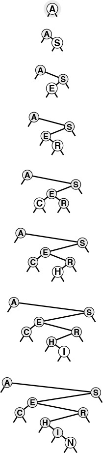
This sequence depicts the result of inserting the keys A S E R C H I N into an initially empty BST. Each insertion follows a search miss at the bottom of the tree.
Figure 12.5 BST construction
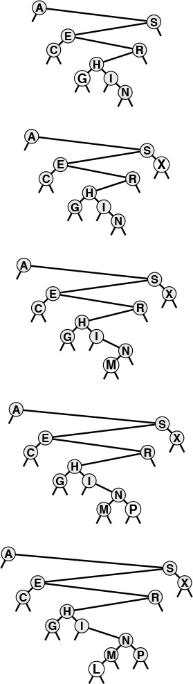
This sequence depicts insertion of the keys G X M P L to the BST started in Figure 12.5.
Figure 12.6 BST construction (continued)
The sort function for symbol tables is available with little extra work when BSTs are used. Constructing a binary search tree amounts to sorting the items, since a binary search tree represents a sorted file when we look at it the right way. In our figures, the keys appear in order if read from left to right on the page (ignoring their height and the links). A program has only the links with which to work, but a simple inorder traversal does the job, by definition, as shown by the recursive implementation sortR in Program 12.8. To visit the items in a BST in order of their keys, we visit the items in the left subtree in order of their keys (recursively), then visit the root, then visit the items in the right subtree in order of their keys (recursively). This deceptively simple implementation is a classic and important recursive program.
Thinking nonrecursively when contemplating search and insert in BSTs is also instructive. In a nonrecursive implementation, the search process consists of a loop where we compare the search key against the key at the root, then move left if the search key is less and right if it is greater. Insertion consists of a search miss (ending in an empty link), then replacement of the empty link with a pointer to a new node. This process corresponds to manipulating the links explicitly along a path down the tree (see Figure 12.4). In particular, to be able to insert a new node at the bottom, we need to maintain a link to the parent of the current node, as in the implementation in Program 12.9. As usual, the recursive and nonrecursive versions are essentially equivalent, but understanding both points of view enhances our understanding of the algorithm and data structure.
The BST functions in Program 12.7 do not explicitly check for items with duplicate keys. When a new node whose key is equal to some key already in the tree is inserted, it falls to the right of the node already in the tree. One side effect of this convention is that nodes with duplicate keys do not appear contiguously in the tree (see Figure 12.7). However, we can find them by continuing the search from the point where STsearch finds the first match, until we encounter z. There are several other options for dealing with items that have duplicate keys, as mentioned in Section 9.1.
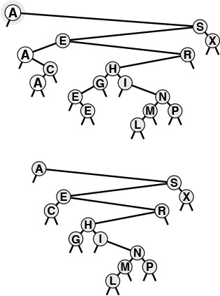
When a BST has records with duplicate keys (top), they appear scattered throughout the tree, as illustrated by the three highlighted A’s. Duplicate keys do all appear on the search path for the key from the root to an external node, so they can readily be accessed. However, to avoid confusing usages such as “the A below the C,” we use distinct keys in our examples (bottom).
Figure 12.7 Duplicate keys in BSTs
BSTs are dual to quicksort. The node at the root of the tree corresponds to the partitioning element in quicksort (no keys to the left are larger, and no keys to the right are smaller). In Section 12.6, we shall see how this observation relates to the analysis of properties of the trees.
Exercises
![]() 12.44 Draw the BST that results when you insert items with the keys E A S Y Q U T I O N, in that order, into an initially empty tree.
12.44 Draw the BST that results when you insert items with the keys E A S Y Q U T I O N, in that order, into an initially empty tree.
![]() 12.45 Draw the BST that results when you insert items with the keys E A S Y Q U E S T I O N, in that order, into an initially empty tree.
12.45 Draw the BST that results when you insert items with the keys E A S Y Q U E S T I O N, in that order, into an initially empty tree.
![]() 12.46 Give the number of comparisons required to put the keys E A S Y Q U E S T I O N into an initially empty symbol table using a BST. Assume that a search is performed for each key, followed by an insert for each search miss, as in Program 12.2.
12.46 Give the number of comparisons required to put the keys E A S Y Q U E S T I O N into an initially empty symbol table using a BST. Assume that a search is performed for each key, followed by an insert for each search miss, as in Program 12.2.
![]() 12.47 Inserting the keys in the order A S E R H I N G C into an initially empty tree also gives the top tree in Figure 12.6. Give ten other orderings of these keys that produce the same result.
12.47 Inserting the keys in the order A S E R H I N G C into an initially empty tree also gives the top tree in Figure 12.6. Give ten other orderings of these keys that produce the same result.
12.48 Implement an STsearchinsert function for binary search trees (Program 12.7). It should search the symbol table for an item with the same key as a given item, then insert the item if it finds none.
![]() 12.49 Write a function that returns the number of items in a BST with keys equal to a given key.
12.49 Write a function that returns the number of items in a BST with keys equal to a given key.
12.50 Suppose that we have an estimate ahead of time of how often search keys are to be accessed in a binary tree. Should the keys be inserted into the tree in increasing or decreasing order of likely frequency of access? Explain your answer.
12.51 Modify the BST implementation in Program 12.7 to keep items with duplicate keys in linked lists hanging from tree nodes. Change the interface to have search operate like sort (for all the items with the search key).
12.52 The nonrecursive insertion procedure in Program 12.9 uses a redundant comparison to determine which link of p to replace with the new node. Give an implementation that uses pointers to links to avoid this comparison.
12.6 Performance Characteristics of BSTs
The running times of algorithms on binary search trees are dependent on the shapes of the trees. In the best case, the tree could be perfectly balanced, with about lg N nodes between the root and each external node, but in the worst case there could be N nodes on the search path.
We might expect the search times also to be logarithmic in the average case, because the first element inserted becomes the root of the tree: If N keys are to be inserted at random, then this element would divide the keys in half (on the average), which would yield logarithmic search times (using the same argument on the subtrees). Indeed, it could happen that a BST would lead to precisely the same comparisons as binary search (see Exercise 12.55). This case would be the best for this algorithm, with guaranteed logarithmic running time for all searches. In a truly random situation, the root is equally likely to be any key, so such a perfectly balanced tree is extremely rare, and we cannot easily keep the tree perfectly balanced after every insertion. However, highly unbalanced trees are also extremely rare for random keys, so the trees are rather well-balanced on the average. In this section, we shall quantify this observation.
Specifically, the path-length and height measures of binary trees that we considered in Section 5.5 relate directly to the costs of searching in BSTs. The height is the worst-case cost of a search, the internal path length is directly related to the cost of search hits, and external path length is directly related to the cost of search misses.
Property 12.6 Search hits require about 2 ln N ≈ 1.39 lg N comparisons, on the average, in a BST built from N random keys.
We regard successive eq and less operations as a single comparison, as discussed in Section 12.3. The number of comparisons used for a search hit ending at a given node is 1 plus the distance from that node to the root. Adding these distances for all nodes, we get the internal path length of the tree. Thus, the desired quantity is 1 plus the average internal path length of the BST, which we can analyze with a familiar argument: If CN denotes the average internal path length of a binary search tree of N nodes, we have the recurrence

with C1 = 1. The N − 1 term takes into account that the root contributes 1 to the path length of each of the other N − 1 nodes in the tree; the rest of the expression comes from observing that the key at the root (the first inserted) is equally likely to be the kth smallest, leaving random subtrees of size k − 1 and N − k. This recurrence is nearly identical to the one that we solved in Chapter 7 for quicksort, and we can solve it in the same way to derive the stated result. ![]()
Property 12.7 Insertions and search misses require about 2 ln N ≈ 1.39 lg N comparisons, on the average, in a BST built from N random keys.
A search for a random key in a tree of N nodes is equally likely to end at any of the N + 1 external nodes on a search miss. This property, coupled with the fact that the difference between the external path length and the internal path length in any tree is merely 2N (see Property 5.7), establishes the stated result. In any BST, the average number of comparisons for an insertion or a search miss is about 1 greater than the average number of comparisons for a search hit. ![]()
Property 12.6 says that we should expect the search cost for BSTs to be about 39% higher than that for binary search for random keys, but Property 12.7 says that the extra cost is well worthwhile, because a new key can be inserted at about the same cost—flexibility not available with binary search. Figure 12.8 shows a BST built from a long random permutation. Although it has some short paths and some long paths, we can characterize it as well balanced: Any search requires less than 12 comparisons, and the average number of comparisons for a random search hit is 7.06, as compared to 5.55 for binary search.
In this BST, which was built by inserting about 200 random keys into an initially empty tree, no search uses more than 12 comparisons. The average cost for a search hit is about 7.
Figure 12.8 Example of a binary search tree
Properties 12.6 and 12.7 are results on average-case performance that depend on the keys being randomly ordered. If the keys are not randomly ordered, the algorithm can perform badly.
Property 12.8 In the worst case, a search in a binary search tree with N keys can require N comparisons.
Figures 12.9 and 12.10 depict two examples of worst-case BSTs. For these trees, binary-tree search is no better than sequential search using singly linked lists. ![]()
If the keys arrive in increasing order at a BST, it degenerates to a form equivalent to a singly linked list, leading to quadratic tree-construction time and linear search time.
Figure 12.9 A worst-case BST
Many other key insertion orders, such as this one, lead to degenerate BSTs. Still, a BST built from randomly ordered keys is likely to be well balanced.
Figure 12.10 Another worst-case BST
Thus, good performance of the basic BST implementation of symbol tables is dependent on the keys being sufficiently similar to random keys that the tree is not likely to contain many long paths. Furthermore, this worst-case behavior is not unlikely in practice—it arises when we insert keys in order or in reverse order into an initially empty tree using the standard algorithm, a sequence of operations that we certainly might attempt without any explicit warnings to avoid doing so. In Chapter 13, we shall examine techniques for making this worst case extremely unlikely and for eliminating it entirely, making all trees look more like best-case trees, with all path lengths guaranteed to be logarithmic.
None of the other symbol-table implementations that we have discussed can be used for the task of inserting a huge number of random keys into a table, then searching for each of them—the running time of each of the methods that we discussed in Sections 12.2 through 12.4 goes quadratic for this task. Furthermore, the analysis tells us that the average distance to a node in a binary tree is proportional to the logarithm of the number of nodes in the tree, which gives us the flexibility to efficiently handle intermixed searches, insertions, and other symbol-table ADT operations, as we shall soon see.
Exercises
![]() 12.53 Write a recursive program that computes the maximum number of comparisons required by any search in a given BST (the height of the tree).
12.53 Write a recursive program that computes the maximum number of comparisons required by any search in a given BST (the height of the tree).
![]() 12.54 Write a recursive program that computes the average number of comparisons required by a search hit in a given BST (the internal path length of the tree divided by N).
12.54 Write a recursive program that computes the average number of comparisons required by a search hit in a given BST (the internal path length of the tree divided by N).
12.55 Give an insertion sequence for the keys E A S Y Q U E S T I O N into an initially empty BST such that the tree produced is equivalent to binary search, in the sense that the sequence of comparisons done in the search for any key in the BST is the same as the sequence of comparisons used by binary search for the same set of keys.
![]() 12.56 Write a program that inserts a set of keys into an initially empty BST such that the tree produced is equivalent to binary search, in the sense described in Exercise 12.55.
12.56 Write a program that inserts a set of keys into an initially empty BST such that the tree produced is equivalent to binary search, in the sense described in Exercise 12.55.
12.57 Draw all the structurally different BSTs that can result when N keys are inserted into an initially empty tree, for 2 ≤ N ≤ 5.
![]() 12.58 Find the probability that each of the trees in Exercise 12.57 is the result of inserting N random distinct elements into an initially empty tree.
12.58 Find the probability that each of the trees in Exercise 12.57 is the result of inserting N random distinct elements into an initially empty tree.
![]() 12.59 How many binary trees of N nodes are there with height N? How many different ways are there to insert N distinct keys into an initially empty tree that result in a BST of height N?
12.59 How many binary trees of N nodes are there with height N? How many different ways are there to insert N distinct keys into an initially empty tree that result in a BST of height N?
![]() 12.60 Prove by induction that the difference between the external path length and the internal path length in any binary tree is 2N (see Property 5.7).
12.60 Prove by induction that the difference between the external path length and the internal path length in any binary tree is 2N (see Property 5.7).
12.61 Run empirical studies to compute the average and standard deviation of the number of comparisons used for search hits and for search misses in a binary search tree built by inserting N random keys into an initially empty tree, for N = 103, 104, 105, and 106.
12.62 Write a program that builds t BSTs by inserting N random keys into an initially empty tree, and that computes the maximum tree height (the maximum number of comparisons involved in any search miss in any of the t trees), for N = 103, 104, 105, and 106 with t = 10, 100, and 1000.
12.7 Index Implementations with Symbol Tables
For many applications we want a search structure simply to help us find items, without moving them around. For example, we might have an array of items with keys, and we might want the search method to give us the index into that array of the item matching a certain key. Or we might want to remove the item with a given index from the search structure, but still keep it in the array for some other use. In Section 9.6, we considered the advantages of processing index items in priority queues, referring to data in a client array indirectly. For symbol tables, the same concept leads to the familiar index: a search structure external to a set of items that provides quick access to items with a given key. In Chapter 16, we shall consider the case where the items and perhaps even the index are in external storage; in this section, we briefly consider the case when both the items and the index fit in memory.
We can adapt binary search trees to build indices in precisely the same manner as we provided indirection for heaps in Section 9.6: use an item’s array index as the item in the BST, and arrange for keys to be extracted from items via the key macro; for example,
#define key(A) realkey(a[A]).
Extending this approach, we can use parallel arrays for the links, as we did for linked lists in Chapter 3. We use three arrays, one each for the items, left links, and right links. The links are array indices (integers), and we replace link references such as
x = x->l
in all our code with array references such as
x = l[x].
This approach avoids the cost of dynamic memory allocation—the items occupy an array without regard to the search function, and we preallocate two integers per item to hold the tree links, recognizing that we will need at least this amount of space when all the items are in the search structure. The space for the links is not always in use, but it is there for use by the search routine without any time overhead for allocation. Another important feature of this approach is that it allows extra arrays (extra information associated with each node) to be added without the tree-manipulation code being changed at all. When the search routine returns the index for an item, it gives a way to access immediately all the information associated with that item, by using the index to access an appropriate array.
This way of implementing BSTs to aid in searching large arrays of items is useful, because it avoids the extra expense of copying items into the internal representation of the ADT, and the overhead of the malloc storage-allocation mechanism. The use of arrays is not appropriate when space is at a premium and the symbol table grows and shrinks markedly, particularly if it is difficult to estimate the maximum size of the symbol table in advance. If no accurate size prediction is possible, unused links might waste space in the item array.
An important application of the indexing concept is to provide keyword searching in a string of text (see Figure 12.11). Program 12.10 is an example of such an application. It reads a text string from an external file. Then, considering each position in the text string to define a string key starting at that position and going to the end of the string, it inserts all the keys into a symbol table, using string pointers as in the string-item type definition in Program 6.11. The string keys used to build the BST are arbitrarily long, but we maintain only pointers to them, and we look at only enough characters to decide whether one string is less than another. No two strings are equal (they are all of different lengths), but if we modify eq to consider two strings to be equal if one is a prefix of the other, we can use the symbol table to find whether a given query string is in the text, simply by calling STsearch. Program 12.10 reads a series of queries from standard input, uses STsearch to determine whether each query is in the text, and prints out the text position of the first occurrence of the query. If the symbol table is implemented with BSTs, then we expect from Property 12.6 that the search will involve about 2N ln N comparisons. For example, once the index is built, we could find any phrase in a text consisting of about 1 million characters (such as Moby Dick) with about 30 string comparisons. This application is the same as indexing, because string pointers are like indices into a character array in C. If p points to text[i], then the difference between the two pointers, p-text, is equal to i.
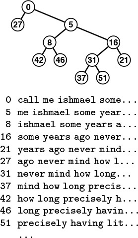
In this example of a string index, we define a string key to begin with each word in a text; then, we build a BST, accessing the keys with their string index. The keys are arbitrarily long in principle, but only a few leading characters are generally examined, in practice. For example, to find out whether the phrase never mind appears in this text, we compare with call... at the root (string index 0), then me... at the right child of the root (index 5), then some... at the right child of that node (index 16), then we find never mind on the left of that node (index 31).
Figure 12.11 Text string index
There are many other issues for us to consider when we are building indices in practical applications, and there are many ways that we can take particular advantage of the properties of string keys to speed up our algorithms. More sophisticated methods for string search and for providing indices with useful capabilities for string keys will be primary topics in Part 5.
Table 12.2 gives empirical results that support the analytic results that we have been examining, and demonstrates the utility of BSTs for dynamic symbol tables with random keys.
This table gives relative times for constructing a symbol table, then searching for each of the keys in the table. BSTs provide fast implementations of search and insertion; all the other methods require quadratic time for one of the two tasks. Binary search is generally slightly faster than BST search, but cannot be used for huge files unless the table can be presorted. The standard BST implementation allocates memory for each tree node, whereas the index implementation preallocates memory for the whole tree (which speeds up construction) and uses array indices instead of pointers (which slows down searching).
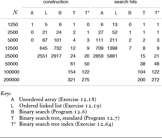
Table 12.2 Empirical study of symbol-table implementations
Exercises
12.63 Modify our BST implementation (Program 12.7) to use an indexed array of items, rather than allocated memory. Compare the performance of your program with that of the standard implementation, using one of the drivers in Exercise 12.21 or Exercise 12.22.
12.64 Modify our BST implementation (Program 12.7) to support a first-class symbol-table ADT with client item handles (see Exercises 12.4 and 12.5), using parallel arrays. Compare the performance of your program with that of the standard implementation, using one of the drivers in Exercise 12.21 or Exercise 12.22.
12.65 Modify our BST implementation (Program 12.7) to use the following idea to represent BSTs: Keep an array of items with keys and an array of links (one associated with each item) in tree nodes. A left link in the BST corresponds to a move to the next position in the array in the tree node, and a right link in the BST corresponds to a move to another tree node.
![]() 12.66 Give an example of a text string where the number of character comparisons for the index-construction part of Program 12.10 is quadratic in the length of the string.
12.66 Give an example of a text string where the number of character comparisons for the index-construction part of Program 12.10 is quadratic in the length of the string.
12.67 Modify our string index implementation (Program 12.10) to use only the keys that start on word boundaries to build the index (see Figure 12.11). (For Moby Dick, this change cuts the size of the index by more than a factor of five.)
![]() 12.68 Implement a version of Program 12.10 that uses binary search on an array of string pointers, using the implementation described in Exercise 12.36.
12.68 Implement a version of Program 12.10 that uses binary search on an array of string pointers, using the implementation described in Exercise 12.36.
12.69 Compare the running time of your implementation from Exercise 12.68 with Program 12.10, to construct an index for a random text string of N characters, for N = 103, 104, 105, and 106, and to do 1000 (unsuccessful) searches for random keys in each index.
12.8 Insertion at the Root in BSTs
In the standard implementation of BSTs, every new node inserted goes somewhere at the bottom of the tree, replacing some external node. This state of affairs is not an absolute requirement; it is just an artifact of the natural recursive insertion algorithm. In this section, we consider an alternative insertion method, where we insist that each new item be inserted at the root, so recently inserted nodes are at the top of the tree. Trees built in this way have some interesting properties, but our main reason for considering this method is that it plays a crucial role in two of the improved BST algorithms that we consider in Chapter 13.
Suppose that the key of the item to be inserted is larger than the key at the root. We might start to make a new tree by putting the new item into a new root node, with the old root as the left subtree and the right subtree of the old root as the right subtree. However, the right subtree may contain some smaller keys, so we need to do more work to complete the insertion. Similarly, if the key of the item to be inserted is smaller than the key at the root and is larger than all the keys in the left subtree of the root, we can again make a new tree with the new item at the root, but more work is needed if the left subtree contains some larger keys. To move all nodes with smaller keys to the left subtree and all nodes with larger keys to the right subtree seems a complicated transformation in general, since the nodes that have to be moved can be scattered along the search path for the node to be inserted.
Fortunately, there is a simple recursive solution to this problem, which is based on rotation, a fundamental transformation on trees. Essentially, a rotation allows us to interchange the role of the root and one of the root’s children in a tree while still preserving the BST ordering among the keys in the nodes. A right rotation involves the root and the left child (see Figure 12.12). The rotation puts the root on the right, essentially reversing the direction of the left link of the root: Before the rotation, it points from the root to the left child; after the rotation, it points from the old left child (the new root) to the old root (the right child of the new root). The tricky part, which makes the rotation work, is to copy the right link of the left child to be the left link of the old root. This link points to all the nodes with keys between the two nodes involved in the rotation. Finally, the link to the old root has to be changed to point to the new root. The description of a left rotation is identical to the description just given, with “right” and “left” interchanged everywhere (see Figure 12.13).
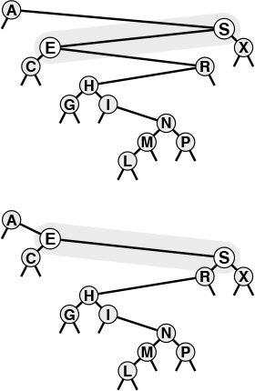
This diagram shows the result (bottom) of a right rotation at S in an example BST (top). The node containing S moves down in the tree, becoming the right child of its former left child.
We accomplish the rotation by getting the link to the new root E from the left link of S, setting the left link of S by copying the right link of E, setting the right link of E to S, and setting the link to S from A to point to E instead.
The effect of the rotation is to move E and its left subtree up one level, and to move S and its right subtree down one level. The rest of the tree is not affected at all.
Figure 12.12 Right rotation in a BST
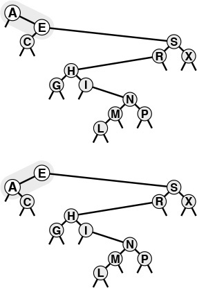
This diagram shows the result (bottom) of a left rotation at A in an example BST (top). The node containing A moves down in the tree, becoming the left child of its former right child.
We accomplish the rotation by getting the link to the new root E from the right link of A, setting the right link of A by copying the left link of E, setting the left link of E to A, and setting the link to A (the head link of the tree) to point to E instead.
Figure 12.13 Left rotation in a BST
A rotation is a local change, involving only three links and two nodes, that allows us to move nodes around in trees without changing the global ordering properties that make BSTs useful for search (see Program 12.11). We use rotations to move specific nodes through a tree and to keep the trees from becoming unbalanced. In Section 12.9 we implement delete, join, and other ADT operations with rotations; in Chapter 13 we use them to help us build trees that afford near-optimal performance.
The rotation operations provide a straightforward recursive implementation of root insertion: Recursively insert the new item into the appropriate subtree (leaving it, when the recursive operation is complete, at the root of that tree), then rotate to make it the root of the main tree. Figure 12.14 depicts an example, and Program 12.12 is a direct implementation of this method. This program is a persuasive example of the power of recursion—any reader not so persuaded is encouraged to try Exercise 12.73.
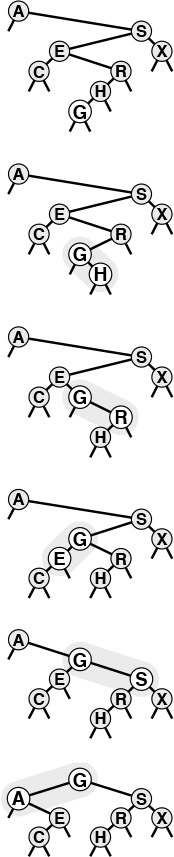
This sequence depicts the result of inserting G into the BST at the top, with (recursive) rotation after insertion to bring the newly inserted node G to the root. The process is equivalent to inserting G, then performing a sequence of rotations to bring it to the root.
Figure 12.14 BST root insertion
Figures 12.15 and 12.16 show how we construct a BST by inserting a sequence of keys into an initially empty tree, using the root insertion method. If the key sequence is random, a BST built in this way has precisely the same stochastic properties as does a BST built by the standard method. For example, Properties 12.6 and 12.7 hold for BSTs built by root insertion.
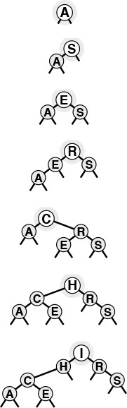
This sequence depicts the result of inserting the keys A S E R C H I into an initially empty BST, using the root insertion method. Each new node is inserted at the root, with links along its search path changed to make a proper BST.
Figure 12.15 BST construction with root insertion
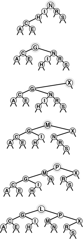
This sequence depicts insertion of the keys N G X M P L to the BST started in Figure 12.15.
Figure 12.16 BST construction with root insertion (continued)
In practice, an advantage of the root insertion method is that recently inserted keys are near the top. The cost for search hits on recently inserted keys therefore is likely to be lower than that for the standard method. This property is significant, because many applications have precisely this kind of dynamic mix among their search and insert operations. A symbol table might contain a great many items, but a large fraction of the searches might refer to the items that were most recently inserted. For example, in a commercial transaction processing system, active transactions could remain near the top and be processed quickly, without access to old transactions being lost. The root insertion method gives the data structure this and similar properties automatically.
If we also change the search function to bring the node found to the root when we have a search hit, then we have a self-organizing search method (see Exercise 12.26) that keeps frequently accessed nodes near the top of the tree. In Chapter 13, we shall see a systematic application of this idea to provide a symbol-table implementation that has guaranteed fast performance characteristics.
As is true of several other methods that we have mentioned in this chapter, it is difficult to make precise statements about the performance of the root insertion method versus the standard insertion method for practical applications, because the performance depends on the mixture of symbol-table operations in a way that is difficult to characterize analytically. Our inability to analyze the algorithm should not necessarily dissuade us from using root insertion when we know that the preponderance of searches are for recently inserted data, but we always seek precise performance guarantees—our main focus in Chapter 13 is methods for constructing BSTs such that these guarantees can be provided.
Exercises
![]() 12.70 Draw the BST that results when you insert items with the keys E A S Y Q U E S T I O N into an initially empty tree, using the root insertion method.
12.70 Draw the BST that results when you insert items with the keys E A S Y Q U E S T I O N into an initially empty tree, using the root insertion method.
12.71 Give a sequence of 10 keys (use the letters A through J) that, when inserted into an initially empty tree via the root insertion method, requires a maximal number of comparisons to build the tree. Give the number of comparisons used.
12.72 Add the code necessary to have Program 12.11 properly modify the count fields that need to be changed after the rotation.
![]() 12.73 Implement a nonrecursive BST root insertion function (see Program 12.12).
12.73 Implement a nonrecursive BST root insertion function (see Program 12.12).
12.74 Run empirical studies to compute the average and standard deviation of the number of comparisons used for search hits and for search misses in a BST built by inserting N random keys into an initially empty tree, then performing a sequence of N random searches for the N/10 most recently inserted keys, for N = 103, 104, 105, and 106. Run your experiment both for the standard insertion method and for the root insertion method; then, compare the results.
12.9 BST Implementations of Other ADT Functions
The recursive implementations given in Section 12.5 for the fundamental search, insert, and sort functions using binary tree structures are straightforward. In this section, we consider implementations of select, join, and delete. One of these, select, also has a natural recursive implementation, but the others can be cumbersome to implement, and can lead to performance problems. The select operation is important to consider because the ability to support select and sort efficiently is one reason that BSTs are preferred over competing structures for many applications. Some programmers avoid using BSTs to avoid having to deal with the delete operation; in this section, we shall see a compact implementation that ties together these operations and uses the rotation-to-the-root technique of Section 12.8.
Generally, the operations involve moving down a path in the tree; so, for random BSTs, we expect the costs to be logarithmic. However, we cannot take for granted that BSTs will stay random when multiple operations are performed on the trees. We shall return to this issue at the end of this section.
To implement select, we can use a recursive procedure that is analogous to the quicksort-based selection method that is described in Section 7.8. In this discussion, as in Section 7.8, we use zero-based indexing, so that, for example, we choose k = 3 to get the item with the fourth smallest key because that one would be in a[3] if the items were in sorted order in the array a. (Some C programmers would insist that the interface be designed in accordance with this convention; others find it confusing to call the smallest key the 0th and the second smallest the 1st, so we leave this question to be resolved differently, if necessary, in different applications.) Now, to find the item with the kth smallest key in a BST, we check the number of nodes in the left subtree. If there are k nodes there, then we return the item at the root. Otherwise, if the left subtree has more than k nodes, we (recursively) look for the item with the kth smallest key there. If neither of these conditions holds, then the left subtree has t items with t < k, and the item with the kth smallest key in the BST is the item with the (k −t−1)st smallest key in the right subtree. Program 12.13 is a direct implementation of this method. As usual, since each execution of the function ends with at most one recursive call, a nonrecursive version is immediate (see Exercise 12.75).
The primary algorithmic reason for including the count field in BST nodes is to support the implementation of select. It also allows us to support a trivial implementation of the count operation (return the count field in the root), and we shall see another use in Chapter 13. The drawbacks to having the count field are that it uses extra space in every node, and that every function that changes the tree needs to update the field. Maintaining the count field may not be worth the trouble in some applications where insert and search are the primary operations, but it might be a small price to pay if it will be important to support the select operation in a dynamic symbol table.
We can change this implementation of the select operation into a partition operation, which rearranges the tree to put the kth smallest element at the root, with precisely the same recursive technique that we used for root insertion in Section 12.8: If we (recursively) put the desired node at the root of one of the subtrees, we can then make it the root of the whole with a single rotation. Program 12.14 gives an implementation of this method. Like rotations, partitioning is not an ADT operation because it is a function that transforms a particular symbol-table representation and should be transparent to clients. Rather, it is an auxiliary routine that we can use to implement ADT operations or to make them run more efficiently. Figure 12.17 depicts an example showing how, in the same way as in Figure 12.14, this process is equivalent to proceeding down the path from the root to the desired node in the tree, then climbing back up, performing rotations to bring the node up to the root.
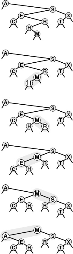
This sequence depicts the result (bottom) of partitioning an example BST (top) about the median key, using (recursive) rotation in the same manner as for root insertion.
Figure 12.17 Partitioning of a BST
To delete a node with a given key from a BST, we first check whether the node is in one of the subtrees. If it is, we replace that subtree with the result of (recursively) deleting the node from it. If the node to be deleted is at the root, we replace the tree with the result of combining the two subtrees into one tree. Several options are available for accomplishing the combination. One approach is illustrated in Figure 12.18, and an implementation is given in Program 12.15. To combine two BSTs with all keys in the second known to be larger than all keys in the first, we apply the partition operation on the second tree, to bring the smallest element in that tree to the root. At this point, the left subtree of the root must be empty (else there would be a smaller element than the one at the root—a contradiction), and we can finish the job by replacing that link with a link to the first tree. Figure 12.19 shows a series of deletions in an example tree, which illustrate some of the situations that can arise.
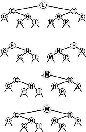
This diagram shows the result (bottom) of deleting the root of an example BST (top). First, we remove the node, leaving two subtrees (second from top). Then, we partition the right subtree to put its smallest element at the root (third from top), leaving the left link pointing to an empty subtree. Finally, we replace this link with a link to the left subtree of the original tree (bottom).
Figure 12.18 Deletion of the root in a BST
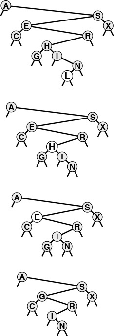
This sequence depicts the result of deleting the nodes with keys L, H, and E from the BST at the top. First, the L is simply removed, since it is at the bottom. Second, the H is replaced with its right child, the I, since the left child of I is empty. Finally, the E is replaced with its successor in the tree, the G.
Figure 12.19 BST node deletion
This approach is asymmetric and is ad hoc in one sense: Why use the smallest key in the second tree as the root for the new tree, rather than the largest key in the first tree? That is, why do we choose to replace the node that we are deleting with the next node in the inorder traversal of the tree, rather than the previous node? We also might want to consider other approaches. For example, if the node to be deleted has a null left link, why not just make its right child the new root, rather than using the node with smallest key in the right subtree? Various similar modifications to the basic delete procedure have been suggested. Unfortunately, they all suffer from a similar flaw: The tree remaining after deletion is not random, even if the tree was random beforehand. Moreover, it has been shown that Program 12.15 tends to leave a tree slightly unbalanced (average height proportional to ![]() ) if the tree is subjected to a large number of random delete–insert pairs (see Exercise 12.81).
) if the tree is subjected to a large number of random delete–insert pairs (see Exercise 12.81).
These differences may not be noticed in practical applications unless N is huge. Still, this combination of an inelegant algorithm with undesirable performance characteristics is unsatisfying. In Chapter 13, we shall examine two different ways to address this situation.
It is typical of search algorithms to require significantly more complicated implementations for deletion than for search. The key values play an integral role in shaping the structure, so removal of a key can involve complicated repairs. One alternative is to use a lazy deletion strategy, leaving deleted nodes in the data structure but marking them as “deleted” so that they can be ignored in searches. In the search implementation in Program 12.7, we can implement this strategy by skipping the equality test for such nodes. We must make sure that large numbers of marked nodes do not lead to excessive waste of time or space, but if deletions are infrequent, the extra cost may not be significant. We could reuse the marked nodes on future insertions when convenient (for example, it would be easy to do so for nodes at the bottom of the tree). Or, we could periodically rebuild the entire data structure, leaving out the marked nodes. These considerations apply to any data structure involving insertions and deletions—they are not peculiar to symbol tables.
We conclude this chapter by considering the implementation of delete with handles and join for first-class symbol-table ADT implementations that use BSTs. We assume that handles are links and omit further discussion about packaging issues, so that we can concentrate on the two basic algorithms.
The primary challenge in implementing a function to delete a node with a given handle (link) is the same as it was for linked lists: We need to change the pointer in the structure that points to the node being deleted. There are at least four ways to address this problem. First, we could add a third link in each tree node, pointing to its parent. The disadvantage of this arrangement is that it is cumbersome to maintain extra links, as we have noted before on several occasions. Second, we could use the key in the item to search in the tree, stopping when we find a matching pointer. This approach suffers from the disadvantage that the average position of a node is near the bottom of the tree, and this approach therefore requires an unnecessary trip through the tree. Third, we could use a pointer to the pointer to the node as the handle. This method is a solution in C, but not in many other languages. Fourth, we could adopt a lazy approach, marking deleted nodes and periodically rebuilding the data structure, as just described.
The last operation for first-class symbol-table ADTs that we need to consider is the join operation. In a BST implementation, this amounts to merging two trees. How do we join two BSTs into one? Various algorithms present themselves to do the job, but each has certain disadvantages. For example, we could traverse the first BST, inserting each of its nodes into the second BST (this algorithm is a one-liner: use STinsert into the second BST as the visit procedure in a STsort of the first BST). This solution does not have linear running time, since each insertion could take linear time. Another idea is to traverse both BSTs, to put the items into an array, to merge them, and then to build a new BST. This operation can be done in linear time, but it also uses a potentially large array.
Program 12.16 is a compact linear-time recursive implementation of the join operation. First, we insert the root of the first BST into the second BST, using root insertion. This operation gives us two subtrees with keys known to be smaller than this root, and two subtrees with keys known to be larger than this root, so we get the result by (recursively) combining the former pair to be the left subtree of the root and the latter to be the right subtree of the root (!). Each node can be the root node on a recursive call at most once, so the total time is linear. An example is shown in Figure 12.20. Like deletion, this process is asymmetric and can lead to trees that are not well balanced, but randomization provides a simple fix, as we shall see in Chapter 13.
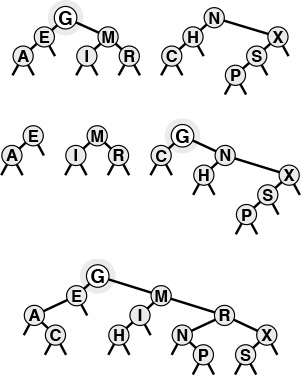
This diagram shows the result (bottom) of combining two example BSTs (top). First, we insert the root G of the first tree into the second tree, using root insertion (second from top). We are left with two subtrees with keys less than G and two subtrees with keys greater than G. Combining both pairs (recursively) gives the result (bottom).
Figure 12.20 Joining of two BSTs
Note that the number of comparisons used for join must be at least linear in the worst case; otherwise we could develop a sorting algorithm that uses fewer than N lg N comparisons, using an approach such as bottom-up mergesort (see Exercise 12.85).
We have not included the code necessary to maintain the count field in BST nodes during the transformations for join and delete, which is necessary for applications where we want to support select (Program 12.13) as well. This task is conceptually simple, but requires some care. One systematic way to proceed is to implement a small utility routine that sets the count field in a node with a value one greater than the sum of the count fields of its children, then call that routine for every node whose links are changed. Specifically, we can do so for both nodes in rotL and rotR in Program 12.11, which suffices for the transformations in Program 12.12 and Program 12.14, since they transform trees solely with rotations. For joinLR and deleteR in Program 12.15 and STjoin in Program 12.16 it suffices to call the node-count update routine for the node to be returned, just before the return statement.
The basic search, insert, and sort operations for BSTs are easy to implement and perform well with even a modicum of randomness in the sequence of operations, so BSTs are widely used for dynamic symbol tables. They also admit simple recursive solutions to support other kinds of operations, as we have seen for select, delete, and join in this chapter, and as we shall see for many examples later in the book.
Despite their utility, there are two primary drawbacks to using BSTs in applications. The first is that they require a substantial amount of space for links. We often think of links and records as being about the same size (say one machine word)—if that is the case, then a BST implementation uses two-thirds of its allocated memory for links and only one-third for keys. This effect is less important in applications with large records and more important in environments where pointers are large. If memory is at a premium, we may prefer one of the open-addressing hashing methods of Chapter 14 to using BSTs.
The second drawback of using BSTs is the distinct possibility that the trees could become poorly balanced and lead to slow performance. In Chapter 13, we examine several approaches to providing performance guarantees. If memory space for links is available, these algorithms make BSTs an attractive choice to serve as the basis for implementation of symbol-table ADTs, because they lead to guaranteed fast performance for a large set of useful ADT operations.
Exercises
![]() 12.75 Implement a nonrecursive BST select function (see Program 12.13).
12.75 Implement a nonrecursive BST select function (see Program 12.13).
![]() 12.76 Draw the BST that results when you insert items with the keys E A S Y Q U T I O N into an initially empty tree, then delete the Q.
12.76 Draw the BST that results when you insert items with the keys E A S Y Q U T I O N into an initially empty tree, then delete the Q.
![]() 12.77 Draw the binary search tree that results when you insert items with the keys EA S Y into one initially empty tree, and insert items with the keys QU E S T I O N into another initially empty tree, then combine the result.
12.77 Draw the binary search tree that results when you insert items with the keys EA S Y into one initially empty tree, and insert items with the keys QU E S T I O N into another initially empty tree, then combine the result.
12.78 Implement a nonrecursive BST delete function (see Program 12.15).
12.79 Implement a version of delete for BSTs (Program 12.15) that deletes all nodes in the tree that have keys equal to the given key.
![]() 12.80 Develop a symbol-table implementation using BSTs that supports the initialize, count, search, insert, delete, join, select, and sort operations for first-class symbol-table ADTs with client item handles (see Exercises 12.4 and 12.5).
12.80 Develop a symbol-table implementation using BSTs that supports the initialize, count, search, insert, delete, join, select, and sort operations for first-class symbol-table ADTs with client item handles (see Exercises 12.4 and 12.5).
12.81 Run experiments to determine how the height of a BST grows as a long sequence of alternating random insertions and deletions is made in a random tree of N nodes, for N = 10, 100, and 1000, and for up to N2 insertion–deletion pairs for each N.
12.82 Implement a version of STdelete (see Program 12.15) that makes a random decision whether to replace the node to be deleted with that node’s predecessor or successor in the tree. Run experiments as described in Exercise 12.81 for this version.
![]() 12.83 Implement a version of
12.83 Implement a version of STdelete that uses a recursive function to move the node to be deleted to the bottom of the tree through rotations, in the manner of root insertion (Program 12.12). Draw the tree produced when your program deletes the root from a complete tree of 31 nodes.
![]() 12.84 Run experiments to determine how the height of a BST grows as you repeatedly reinsert the item at the root into the tree that results when you combine the subtrees of the root in a random tree of N nodes, for N = 10, 100, and 1000.
12.84 Run experiments to determine how the height of a BST grows as you repeatedly reinsert the item at the root into the tree that results when you combine the subtrees of the root in a random tree of N nodes, for N = 10, 100, and 1000.
![]() 12.85 Implement a version of bottom-up mergesort based on the join operation: Start by putting keys into N one-node trees, then combine the one-node trees in pairs to get N/2 two-node trees, then combine the two-node trees in pairs to get N/4 four-node trees, and so forth.
12.85 Implement a version of bottom-up mergesort based on the join operation: Start by putting keys into N one-node trees, then combine the one-node trees in pairs to get N/2 two-node trees, then combine the two-node trees in pairs to get N/4 four-node trees, and so forth.
12.86 Implement a version of STjoin (see Program 12.16) that makes a random decision whether to use the root of the first tree or the root of the second tree for root of the result tree. Run experiments as described in Exercise 12.84 for this version.