Chapter Three. Elementary Data Structures
Organizing the data for processing is an essential step in the development of a computer program. For many applications, the choice of the proper data structure is the only major decision involved in the implementation: once the choice has been made, the necessary algorithms are simple. For the same data, some data structures require more or less space than others; for the same operations on the data, some data structures lead to more or less efficient algorithms than others. The choices of algorithm and of data structure are closely intertwined, and we continually seek ways to save time or space by making the choice properly.
A data structure is not a passive object: We also must consider the operations to be performed on it (and the algorithms used for these operations). This concept is formalized in the notion of a data type. In this chapter, our primary interest is in concrete implementations of the fundamental approaches that we use to structure data. We consider basic methods of organization and methods for manipulating data, work through a number of specific examples that illustrate the benefits of each, and discuss related issues such as storage management. In Chapter 4, we discuss abstract data types, where we separate the definitions of data types from implementations.
We discuss properties of arrays, linked lists, and strings. These classical data structures have widespread applicability: with trees (see Chapter 5), they form the basis for virtually all the algorithms considered in this book. We consider various primitive operations for manipulating these data structures, to develop a basic set of tools that we can use to develop sophisticated algorithms for difficult problems.
The study of storing data as variable-sized objects and in linked data structures requires an understanding of how the system manages the storage that it allocates to programs for their data. We do not cover this subject exhaustively because many of the important considerations are system and machine dependent. However, we do discuss approaches to storage management and several basic underlying mechanisms. Also, we discuss the specific (stylized) manners in which we will be using C storage-allocation mechanisms in our programs.
At the end of the chapter, we consider several examples of compound structures, such as arrays of linked lists and arrays of arrays. The notion of building abstract mechanisms of increasing complexity from lower-level ones is a recurring theme throughout this book. We consider a number of examples that serve as the basis for more advanced algorithms later in the book.
The data structures that we consider in this chapter are important building blocks that we can use in a natural manner in C and many other programming languages. In Chapter 5, we consider another important data structure, the tree. Arrays, strings, linked lists, and trees are the basic elements underlying most of the algorithms that we consider in this book. In Chapter 4, we discuss the use of the concrete representations developed here in building basic abstract data types that can meet the needs of a variety of applications. In the rest of the book, we develop numerous variations of the basic tools discussed here, trees, and abstract data types, to create algorithms that can solve more difficult problems and that can serve us well as the basis for higher-level abstract data types in diverse applications.
3.1 Building Blocks
In this section, we review the primary low-level constructs that we use to store and process information in C. All the data that we process on a computer ultimately decompose into individual bits, but writing programs that exclusively process bits would be tiresome indeed. Types allow us to specify how we will use particular sets of bits and functions allow us to specify the operations that we will perform on the data. We use C structures to group together heterogeneous pieces of information, and we use pointers to refer to information indirectly. In this section, we consider these basic C mechanisms, in the context of presenting a general approach to organizing our programs. Our primary goal is to lay the groundwork for the development, in the rest of the chapter and in Chapters 4 and 5, of the higher-level constructs that will serve as the basis for most of the algorithms that we consider in this book.
We write programs that process information derived from mathematical or natural-language descriptions of the world in which we live; accordingly, computing environments need to provide built-in support for the basic building blocks of such descriptions—numbers and characters. In C, our programs are all built from just a few basic types of data:
• Integers (ints).
• Floating-point numbers (floats).
• Characters (chars).
It is customary to refer to these basic types by their C names—int, float, and char—although we often use the generic terminology integer, floating-point number, and character, as well. Characters are most often used in higher-level abstractions—for example to make words and sentences—so we defer consideration of character data to Section 3.6 and look at numbers here.
We use a fixed number of bits to represent numbers, so ints are by necessity integers that fall within a specific range that depends on the number of bits that we use to represent them. Floating-point numbers approximate real numbers, and the number of bits that we use to represent them affects the precision with which we can approximate a real number. In C, we trade space for accuracy by choosing from among the types int, long int, or short int for integers and from among float or double for floating-point numbers. On most systems, these types correspond to underlying hardware representations. The number of bits used for the representation, and therefore the range of values (in the case of ints) or precision (in the case of floats), is machine-dependent (see Exercise 3.1), although C provides certain guarantees. In this book, for clarity, we normally use int and float, except in cases where we want to emphasize that we are working with problems where big numbers are needed.
In modern programming, we think of the type of the data more in terms of the needs of the program than the capabilities of the machine, primarily, in order to make programs portable. Thus, for example, we think of a short int as an object that can take on values between –32,768 and 32,767, instead of as a 16-bit object. Moreover, our concept of an integer includes the operations that we perform on them: addition, multiplication, and so forth.
Definition 3.1 A data type is a set of values and a collection of operations on those values.
Operations are associated with types, not the other way around. When we perform an operation, we need to ensure that its operands and result are of the correct type. Neglecting this responsibility is a common programming error. In some situations, C performs implicit type conversions; in other situations, we use casts, or explicit type conversions. For example, if x and N are integers, the expression
((float) x) / N
includes both types of conversion: the (float) is a cast that converts the value of x to floating point; then an implicit conversion is performed for N to make both arguments of the divide operator floating point, according to C’s rules for implicit type conversion.
Many of the operations associated with standard data types (for example, the arithmetic operations) are built into the C language. Other operations are found in the form of functions that are defined in standard function libraries; still others take form in the C functions that we define in our programs (see Program 3.1). That is, the concept of a data type is relevant not just to integer, floating point, and character built-in types. We often define our own data types, as an effective way of organizing our software. When we define a simple function in C, we are effectively creating a new data type, with the operation implemented by that function added to the operations defined for the types of data represented by its arguments. Indeed, in a sense, each C program is a data type—a list of sets of values (built-in or other types) and associated operations (functions). This point of view is perhaps too broad to be useful, but we shall see that narrowing our focus to understand our programs in terms of data types is valuable.
One goal that we have when writing programs is to organize them such that they apply to as broad a variety of situations as possible. The reason for adopting such a goal is that it might put us in the position of being able to reuse an old program to solve a new problem, perhaps completely unrelated to the problem that the program was originally intended to solve. First, by taking care to understand and to specify precisely which operations a program uses, we can easily extend it to any type of data for which we can support those operations. Second, by taking care to understand and to specify precisely what a program does, we can add the abstract operation that it performs to the operations at our disposal in solving new problems.
Program 3.2 implements a simple computation on numbers using a simple data type defined with a typedef operation and a function (which itself is implemented with a library function). The main function refers to the data type, not the built-in type of the number. By not specifying the type of the numbers that the program processes, we extend its potential utility. For example, this practice is likely to extend the useful lifetime of a program. When some new circumstance (a new application, or perhaps a new compiler or computer), presents us with a new type of number with which we would like to work, we can update our program just by changing the data type.
This example does not represent a fully general solution to the problem of developing a type-independent program for computing averages and standard deviations—nor is it intended to do so. For example, the program depends on converting a number of type Number to a float to be included in the running average and variance, so we might add that conversion as an operation to the data type, rather than depend on the (float) cast, which only works for built-in types of numbers.
If we were to try to do operations other than arithmetic operations, we would soon find the need to add more operations to the data type. For example, we might want to print the numbers, which would require that we implement, say, a printNum function. Such a function would be less convenient than using the built-in format conversions in printf. Whenever we strive to develop a data type based on identifying the operations of importance in a program, we need to strike a balance between the level of generality that we choose and the ease of implementation and use that results.
It is worthwhile to consider in detail how we might change the data type to make Program 3.2 work with other types of numbers, say floats, rather than with ints. There are a number of different mechanisms available in C that we could use to take advantage of the fact that we have localized references to the type of the data. For such a small program, the simplest is to make a copy of the file, then to change the typedef to
This program computes the average μ and standard deviation σ of a sequence x1, x2, ..., xN of integers generated by the library procedure rand, following the mathematical definitions
Note that a direct implementation from the definition of σ2 requires one pass to compute the average and another to compute the sums of the squares of the differences between the members of the sequence and the average, but rearranging the formula makes it possible for us to compute σ2 in one pass through the data.
We use the typedef declaration to localize reference to the fact that the type of the data is int. For example, we could keep the typedef and the function randNum in a separate file (referenced by an include directive), and then we could use this program to test random numbers of a different type by changing that file (see text).
Whatever the type of the data, the program uses ints for indices and floats to compute the average and standard deviation, and will be effective only if conversion functions from the data to float perform in a reasonable manner.
#include <math.h>
#include <stdlib.h>
#include <stdio.h>
typedef int Number;
Number randNum()
{ return rand(); }
main(int argc, char *argv[])
{ int i, N = atoi(argv[1]);
float m1 = 0.0, m2 = 0.0;
Number x;
for (i = 0; i < N; i++)
{
x = randNum();
m1 += ((float) x)/N;
m2 += ((float) x*x)/N;
}
printf(" Average: %f
", m1);
printf("Std. deviation: %f
", sqrt(m2-m1*m1));
}
and the function randNum to
return 1.0*rand()/RAND_MAX;
(which will return random floating-point numbers between 0 and 1). Even for such a small program, this approach is inconvenient because it leaves us with two copies of the main program, and we will have to make sure that any later changes in that program are reflected in both copies. In C, an alternative approach is to put the typedef and randNum into a separate header file—called, say, Num.h—replacing them with the directive
#include "Num.h"
in the code in Program 3.2. Then, we can make a second header file with different typedef and randNum, and, by renaming one of these files or the other Num.h, use the main program in Program 3.2 with either, without modifying it at all.
A third alternative, which is recommended software engineering practice, is to split the program into three files:
• An interface, which defines the data structure and declares the functions to be used to manipulate the data structure
• An implementation of the functions declared in the interface
• A client program that uses the functions declared in the interface to work at a higher level of abstraction
With this arrangement, we can use the main program in Program 3.2 with integers or floats, or extend it to work with other data types, just by compiling it together with the specific code for the data type of interest. Next, we shall consider the precise change that we need to convert Program 3.2 into a more flexible implementation, using this approach.
We think of the interface as a definition of the data type. It is a contract between the client program and the implementation program. The client agrees to access the data only through the functions defined in the interface, and the implementation agrees to deliver the promised functions.
For the example in Program 3.2, the interface would consist of the declarations
typedef int Number;
Number randNum();
The first line specifies the type of the data to be processed, and the second specifies an operation associated with the type. This code might be kept, for example, in a file named Num.h.
The implementation of the interface in Num.h is an implementation of the randNum function, which might consist of the code
#include <stdlib.h>
#include "Num.h"
Number randNum()
{ return rand(); }
The first line refers to the system-supplied interface that describes the rand() function; the second line refers to the interface that we are implementing (we include it as a check that the function we are implementing is the same type as the one that we declared), and the final two lines give the code for the function. This code might be kept, for example, in a file named int.c. The actual code for the rand function is kept in the standard C run-time library.
A client program corresponding to Program 3.2 would begin with the include directives for interfaces that declare the functions that it uses, as follows:
#include <stdio.h>
#include <math.h>
#include "Num.h"
The function main from Program 3.2 then can follow these three lines. This code might be kept, for example, in a file named avg.c.
Compiled together, the programs avg.c and int.c described in the previous paragraphs have the same functionality as Program 3.2, but they represent a more flexible implementation both because the code associated with the data type is encapsulated and can be used by other client programs and because avg.c can be used with other data types without being changed.
There are many other ways to support data types besides the client–interface–implementation scenario just described, but we will not dwell on distinctions among various alternatives because such distinctions are best drawn in a systems-programming context, rather than in an algorithm-design context (see reference section). However, we do often make use of this basic design paradigm because it provides us with a natural way to substitute improved implementations for old ones, and therefore to compare different algorithms for the same applications problem. Chapter 4 is devoted to this topic.
We often want to build data structures that allow us to handle collections of data. The data structures may be huge, or they may be used extensively, so we are interested in identifying the important operations that we will perform on the data and in knowing how to implement those operations efficiently. Doing these tasks is taking the first steps in the process of incrementally building lower-level abstractions into higher-level ones; that process allows us to conveniently develop ever more powerful programs. The simplest mechanisms for grouping data in an organized way in C are arrays, which we consider in Section 3.2, and structures, which we consider next.
Structures are aggregate types that we use to define collections of data such that we can manipulate an entire collection as a unit, but can still refer to individual components of a given datum by name. Structures are not at the same level as built-in types such as int or float in C, because the only operations that are defined for them (beyond referring to their components) are copy and assignment. Thus, we can use a structure to define a new type of data, and can use it to name variables, and can pass those variables as arguments to functions, but we have specifically to define as functions any operations that we want to perform.
For example, when processing geometric data we might want to work with the abstract notion of points in the plane. Accordingly, we can write
struct point { float x; float y; };
to indicate that we will use type point to refer to pairs of floating-point numbers. For example, the statement
struct point a, b;
declares two variables of this type. We can refer to individual members of a structure by name. For example, the statements
a.x = 1.0; a.y = 1.0; b.x = 4.0; b.y = 5.0;
set a to represent the point (1, 1) and b to represent the point (4, 5).
We can also pass structures as arguments to functions. For example, the code
float distance(struct point a, struct point b)
{ float dx = a.x - b.x, dy = a.y - b.y;
return sqrt(dx*dx + dy*dy);
}
defines a function that computes the distance between two points in the plane. This example illustrates the natural way in which structures allow us to aggregate our data in typical applications.
Program 3.3 is an interface that embodies the definition of a data type for points in the plane, uses a structure to represent the points, and includes an operation to compute the distance between two points. Program 3.4 is a function that implements the operation. We use interface-implementation arrangements like this to define data types whenever possible, because they encapsulate the definition (in the interface) and the implementation in a clear and direct manner. We make use of the data type in a client program by including the interface and by compiling the implementation with the client program (or by using appropriate separate-compilation facilities). Program 3.4 uses a typedef to define the point data type so that client programs can declare points as point instead of struct point, and do not have to make any assumptions about how the data types are represented. In Chapter 4, we shall see how to carry this separation between client and implementation one step further.
We cannot use Program 3.2 to process items of type point because arithmetic and type conversion operations are not defined for points. Modern languages such as C++ and Java have basic constructs that make it possible to use previously defined high-level abstract operations, even for newly defined types. With a sufficiently general interface, we could make these arrangements, even in C. In this book, however, although we strive to develop interfaces of general utility, we resist obscuring our algorithms or sacrificing good performance for that reason. Our primary goal is to make clear the effectiveness of the algorithmic ideas that we will be considering. Although we often stop short of a fully general solution, we do pay careful attention to the process of precisely defining the abstract operations that we want to perform, as well as the data structures and algorithms that will support those operations, because doing so is at the heart of developing efficient and effective programs. We will return to this issue, in detail, in Chapter 4.
The point structure example just given is a simple one that comprises two items of the same type. In general, structures can mix different types of data. We shall be working extensively with such structures throughout the rest of this chapter.
Beyond giving us the specific basic types int, float, and char, and the ability to build them into compound types with struct, C provides us with the ability to manipulate our data indirectly. A pointer is a reference to an object in memory (usually implemented as a machine address). We declare a variable a to be a pointer to (for example) an integer by writing int *a, and we can refer to the integer itself as *a. We can declare pointers to any type of data. The unary operator & gives the machine address of an object, and is useful for initializing pointers. For example, *&a is the same as a. We restrict ourselves to using & for this purpose, as we prefer to work at a somewhat higher level of abstraction than machine addresses when possible.
Referring to an object indirectly via a pointer is often more convenient than referring directly to the object, and can also be more efficient, particularly for large objects. We will see many examples of this advantage in Sections 3.3 through 3.7. Even more important, as we shall see, we can use pointers to structure our data in ways that support efficient algorithms for processing the data. Pointers are the basis for many data structures and algorithms.
A simple and important example of the use of pointers arises when we consider the definition of a function that is to return multiple values. For example, the following function (using the functions sqrt and atan2 from the standard library) converts from Cartesian to polar coordinates:
polar(float x, float y, float *r, float *theta)
{
*r = sqrt(x*x + y*y);
*theta = atan2(y, x);
}
In C, all function arguments are passed by value—if the function assigns a new value to an argument variable, that assignment is local to the function and is not seen by the calling program. This function therefore cannot change the pointers to the floating-point numbers r and theta, but it can change the values of the numbers, by indirect reference. For example, if a calling program has a declaration float a, b, the function call
polar(1.0, 1.0, &a, &b)
will result in a being set to 1.414214 (![]() ) and
) and b being set to 0.785398 (π/4). The & operator allows us to pass the addresses of a and b to the function, which treats those arguments as pointers. We have already seen an example of this usage, in the scanf library function.
So far, we have primarily talked about defining individual pieces of information for our programs to process. In many instances, we are interested in working with potentially huge collections of data, and we now turn to basic methods for doing so. In general, we use the term data structure to refer to a mechanism for organizing our information to provide convenient and efficient mechanisms for accessing and manipulating it. Many important data structures are based on one or both of the two elementary approaches that we shall consider in this chapter. We may use an array, where we organize objects in a fixed sequential fashion that is more suitable for access than for manipulation; or a list, where we organize objects in a logical sequential fashion that is more suitable for manipulation than for access.
Exercises
![]() 3.1 Find the largest and smallest numbers that you can represent with types
3.1 Find the largest and smallest numbers that you can represent with types int, long int, short int, float, and double in your programming environment.
3.2 Test the random-number generator on your system by generating N random integers between 0 and r – 1 with rand() % r and computing the average and standard deviation for r = 10, 100, and 1000 and N = 103, 104, 105, and 106.
3.3 Test the random-number generator on your system by generating N random numbers of type double between 0 and 1, transforming them to integers between 0 and r – 1 by multiplying by r and truncating the result, and computing the average and standard deviation for r = 10, 100, and 1000 and N = 103, 104, 105, and 106.
![]() 3.4 Do Exercises 3.2 and 3.3 for r = 2, 4, and 16.
3.4 Do Exercises 3.2 and 3.3 for r = 2, 4, and 16.
3.5 Implement the necessary functions to allow Program 3.2 to be used for random bits (numbers that can take only the values 0 or 1).
3.6 Define a struct suitable for representing a playing card.
3.7 Write a client program that uses the data type in Programs 3.3 and 3.4 for the following task: Read a sequence of points (pairs of floating-point numbers) from standard input, and find the one that is closest to the first.
![]() 3.8 Add a function to the point data type (Programs 3.3 and 3.4) that determines whether or not three points are collinear, to within a numerical tolerance of 10–4. Assume that the points are all in the unit square.
3.8 Add a function to the point data type (Programs 3.3 and 3.4) that determines whether or not three points are collinear, to within a numerical tolerance of 10–4. Assume that the points are all in the unit square.
3.9 Define a data type for points in the plane that is based on using polar coordinates instead of Cartesian coordinates.
![]() 3.10 Define a data type for triangles in the unit square, including a function that computes the area of a triangle. Then write a client program that generates random triples of pairs of
3.10 Define a data type for triangles in the unit square, including a function that computes the area of a triangle. Then write a client program that generates random triples of pairs of floats between 0 and 1 and computes empirically the average area of the triangles generated.
3.2 Arrays
Perhaps the most fundamental data structure is the array, which is defined as a primitive in C and in most other programming languages. We have already seen the use of an array as the basis for the development of an efficient algorithm, in the examples in Chapter 1; we shall see many more examples in this section.
An array is a fixed collection of same-type data that are stored contiguously and that are accessible by an index. We refer to the ith element of an array a as a[i]. It is the responsibility of the programmer to store something meaningful in an array position a[i] before referring to a[i]. In C, it is also the responsibility of the programmer to use indices that are nonnegative and smaller than the array size. Neglecting these responsibilities are two of the more common programming mistakes.
Arrays are fundamental data structures in that they have a direct correspondence with memory systems on virtually all computers. To retrieve the contents of a word from memory in machine language, we provide an address. Thus, we could think of the entire computer memory as an array, with the memory addresses corresponding to array indices. Most computer-language processors translate programs that involve arrays into efficient machine-language programs that access memory directly, and we are safe in assuming that an array access such as a[i] translates to just a few machine instructions.
A simple example of the use of an array is given by Program 3.5, which prints out all prime numbers less than 10000. The method used, which dates back to the third century B.C., is called the sieve of Eratosthenes (see Figure 3.1). It is typical of algorithms that exploit the fact that we can access efficiently any item of an array, given that item’s index. The implementation has four loops, three of which access the items of the array sequentially, from beginning to end; the fourth skips through the array, i items at a time. In some cases, sequential processing is essential; in other cases, sequential ordering is used because it is as good as any other. For example, we could change the first loop in Program 3.5 to
for (a[1] = 0, i = N-1; i > 1; i--) a[i] = 1;
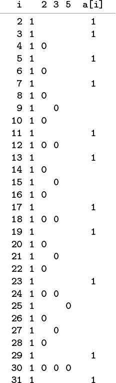
To compute the prime numbers less than 32, we initialize all the array entries to 1 (second column), to indicate that no numbers are known to be nonprime (a[0] and a[1] are not used and are not shown). Then, we set array entries whose indices are multiples of 2, 3, and 5 to 0, since we know these multiples to be nonprime. Indices corresponding to array entries that remain 1 are prime (rightmost column).
Figure 3.1 Sieve of Eratosthenes
without any effect on the computation. We could also reverse the order of the inner loop in a similar manner, or we could change the final loop to print out the primes in decreasing order, but we could not change the order of the outer loop in the main computation, because it depends on all the integers less than i being processed before a[i] is tested for being prime.
We will not analyze the running time of Program 3.5 in detail because that would take us astray into number theory, but it is clear that the running time is proportional to
N + N/2 + N/3 + N/5 + N/7 + N/11 + ...
which is less than N + N/2 + N/3 + N/4 + ... = NHN ~ N ln N.
One of the distinctive features of C is that an array name generates a pointer to the first element of the array (the one with index 0). Moreover, simple pointer arithmetic is allowed: if p is a pointer to an object of a certain type, then we can write code that assumes that objects of that type are arranged sequentially, and can use *p to refer to the first object, *(p+1) to refer to the second object, *(p+2) to refer to the third object, and so forth. In other words,
*(a+i) and a[i] are equivalent in C.
This equivalence provides an alternate mechanism for accessing objects in arrays that is sometimes more convenient than indexing. This mechanism is most often used for arrays of characters (strings); we discuss it again in Section 3.6.
Like structures, pointers to arrays are significant because they allow us to manipulate the arrays efficiently as higher-level objects. In particular, we can pass a pointer to an array as an argument to a function, thus enabling that function to access objects in the array without having to make a copy of the whole array. This capability is indispensable when we write programs to manipulate huge arrays. For example, the search functions that we examined in Section 2.6 use this feature. We shall see other examples in Section 3.7.
The implementation in Program 3.5 assumes that the size of the array must be known beforehand: to run the program for a different value of N, we must change the constant N and recompile the program before executing it. Program 3.6 shows an alternate approach, where a user of the program can type in the value of N, and it will respond with the primes less than N. It uses two basic C mechanisms, both of which involve passing arrays as arguments to functions. The first is the mechanism by which command-line arguments are passed to the main program, in an array argv of size argc. The array argv is a compound array made up of objects that are arrays (strings) themselves, so we shall defer discussing it in further detail until Section 3.7, and shall take on faith for the moment that the variable N gets the number that the user types when executing the program.
The second basic mechanism that we use in Program 3.6 is malloc, a function that allocates the amount of memory that we need for our array at execution time, and returns, for our exclusive use, a pointer to the array. In some programming languages, it is difficult or impossible to allocate arrays dynamically; in some other programming languages, memory allocation is an automatic mechanism. Dynamic allocation is an essential tool in programs that manipulate multiple arrays, some of which might have to be huge. In this case, without memory allocation, we would have to predeclare an array as large as any value that the user is allowed to type. In a large program where we might use many arrays, it is not feasible to do so for each array. We will generally use code like Program 3.6 in this book because of the flexibility that it provides, although in specific applications when the array size is known, simpler versions like Program 3.5 are perfectly suitable. If the array size is fixed and huge, the array may need to be global in some systems. We discuss several of the mechanisms behind memory allocation in Section 3.5, and we look at a way to use malloc to support an abstract dynamic growth facility for arrays in Section 14.5. As we shall see, however, such mechanisms have associated costs, so we generally regard arrays as having the characteristic property that, once allocated, their sizes are fixed, and cannot be changed.
Not only do arrays closely reflect the low-level mechanisms for accessing data in memory on most computers, but also they find widespread use because they correspond directly to natural methods of organizing data for applications. For example, arrays also correspond directly to vectors, the mathematical term for indexed lists of objects.
Program 3.7 is an example of a simulation program that uses an array. It simulates a sequence of Bernoulli trials, a familiar abstract concept from probability theory. If we flip a coin N times, the probability that we see k heads is

The approximation is known as the normal approximation: the familiar bell-shaped curve. Figure 3.2 illustrates the output of Program 3.7 for 1000 trials of the experiment of flipping a coin 32 times. Many more details on the Bernoulli distribution and the normal approximation can be found in any text on probability, and we shall encounter these distributions again in Chapter 13. In the present context, our interest in the computation is that we use the numbers as indices into an array to count their frequency of occurrence. The ability of arrays to support this kind of operation is one of their prime virtues.
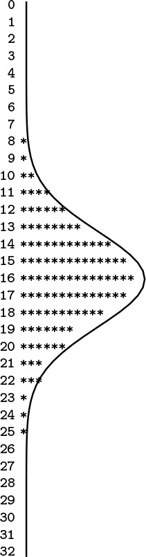
This table shows the result of running Program 3.7 with N = 32 and M = 1000, simulating 1000 experiments of flipping a coin 32 times. The number of heads that we should see is approximated by the normal distribution function, which is drawn over the data.
Figure 3.2 Coin-flipping simulation
Programs 3.5 and 3.7 both compute array indices from the data at hand. In a sense, when we use a computed value to access an array of size N, we are taking N possibilities into account with just a single operation. This gain in efficiency is compelling when we can realize it, and we shall be encountering algorithms throughout the book that make use of arrays in this way.
We use arrays to organize all different manner of types of objects, not just integers. In C, we can declare arrays of any built-in or user-defined type (i.e., compound objects declared as structures). Program 3.8 illustrates the use of an array of structures for points in the plane using the structure definition that we considered in Section 3.1. This program also illustrates a common use of arrays: to save data away so that they can be quickly accessed in an organized manner in some computation. Incidentally, Program 3.8 is also interesting as a prototypical quadratic algorithm, which checks all pairs of a set of N data items, and therefore takes time proportional to N2. In this book, we look for improvements whenever we see such an algorithm, because its use becomes infeasible as N grows. In this case, we shall see how to use a compound data structure to perform this computation in linear time, in Section 3.7.
We can create compound types of arbitrary complexity in a similar manner: We can have not just arrays of structs, but also arrays of arrays, or structs containing arrays. We will consider these different options in detail in Section 3.7. Before doing so, however, we will examine linked lists, which serve as the primary alternative to arrays for organizing collections of objects.
Exercises
![]() 3.11 Suppose that
3.11 Suppose that a is declared as int a[99]. Give the contents of the array after the following two statements are executed:
for (i = 0; i < 99; i++) a[i] = 98-i;
for (i = 0; i < 99; i++) a[i] = a[a[i]];
3.12 Modify our implementation of the sieve of Eratosthenes (Program 3.5) to use an array of (i) chars; and (ii) bits. Determine the effects of these changes on the amount of space and time used by the program.
![]() 3.13 Use the sieve of Eratosthenes to determine the number of primes less than N, for N = 103, 104, 105, and 106.
3.13 Use the sieve of Eratosthenes to determine the number of primes less than N, for N = 103, 104, 105, and 106.
![]() 3.14 Use the sieve of Eratosthenes to draw a plot of N versus the number of primes less than N for N between 1 and 1000.
3.14 Use the sieve of Eratosthenes to draw a plot of N versus the number of primes less than N for N between 1 and 1000.
3.15 Empirically determine the effect of removing the test if (a[i]) that guards the inner loop of Program 3.5, for N = 103, 104, 105, and 106.
![]() 3.16 Analyze Program 3.5 to explain the effect that you observed in Exercise 3.15.
3.16 Analyze Program 3.5 to explain the effect that you observed in Exercise 3.15.
![]() 3.17 Write a program that counts the number of different integers less than 1000 that appear in an input stream.
3.17 Write a program that counts the number of different integers less than 1000 that appear in an input stream.
![]() 3.18 Write a program that determines empirically the number of random positive integers less than 1000 that you can expect to generate before getting a repeated value.
3.18 Write a program that determines empirically the number of random positive integers less than 1000 that you can expect to generate before getting a repeated value.
![]() 3.19 Write a program that determines empirically the number of random positive integers less than 1000 that you can expect to generate before getting each value at least once.
3.19 Write a program that determines empirically the number of random positive integers less than 1000 that you can expect to generate before getting each value at least once.
3.20 Modify Program 3.7 to simulate a situation where the coin turns up heads with probability p. Run 1000 trials for an experiment with 32 flips with p = 1/6 to get output that you can compare with Figure 3.2.
3.21 Modify Program 3.7 to simulate a situation where the coin turns up heads with probability λ/N. Run 1000 trials for an experiment with 32 flips to get output that you can compare with Figure 3.2. This distribution is the classical Poisson distribution.
![]() 3.22 Modify Program 3.8 to print out the coordinates of the closest pair of points.
3.22 Modify Program 3.8 to print out the coordinates of the closest pair of points.
![]() 3.23 Modify Program 3.8 to perform the same computation in d dimensions.
3.23 Modify Program 3.8 to perform the same computation in d dimensions.
3.3 Linked Lists
When our primary interest is to go through a collection of items sequentially, one by one, we can organize the items as a linked list: a basic data structure where each item contains the information that we need to get to the next item. The primary advantage of linked lists over arrays is that the links provide us with the capability to rearrange the items efficiently. This flexibility is gained at the expense of quick access to any arbitrary item in the list, because the only way to get to an item in the list is to follow links, one node to the next. There are a number of ways to organize linked lists, all starting with the following basic definition.
Definition 3.2 A linked list is a set of items where each item is part of a node that also contains a link to a node.
We define nodes in terms of references to nodes, so linked lists are sometimes referred to as self-referent structures. Moreover, although a node’s link usually refers to a different node, it could refer to the node itself, so linked lists can also be cyclic structures. The implications of these two facts will become apparent as we begin to consider concrete representations and applications of linked lists.
Normally, we think of linked lists as implementing a sequential arrangement of a set of items: Starting at a given node, we consider its item to be first in the sequence. Then, we follow its link to another node, which gives us an item that we consider to be second in the sequence, and so forth. In principle, the list could be cyclic and the sequence could seem infinite, but we most often work with lists that correspond to a simple sequential arrangement of a finite set of items, adopting one of the following conventions for the link in the final node:
• It is a null link that points to no node.
• It refers to a dummy node that contains no item.
• It refers back to the first node, making the list a circular list.
In each case, following links from the first node to the final one defines a sequential arrangement of items. Arrays define a sequential ordering of items as well; in an array, however, the sequential organization is provided implicitly, by the position in the array. (Arrays also support arbitrary access by index, which lists do not.)
We first consider nodes with precisely one link, and, in most applications, we work with one-dimensional lists where all nodes except possibly the first one and the final one each have precisely one link referring to them. This corresponds to the simplest situation, which is also the one that interests us most, where linked lists correspond to finite sequences of items. We will consider more complicated situations in due course.
Linked lists are defined as a primitive in some programming environments, but not in C. However, the basic building blocks that we discussed in Section 3.1 are well suited to implementing linked lists. Specifically, we use pointers for links and structures for nodes. The typedef declaration gives us a way to refer to links and nodes, as follows:
typedef struct node *link;
struct node { Item item; link next; };
which is nothing more than C code for Definition 3.2. Links are pointers to nodes, and nodes consist of items and links. We assume that another part of the program uses typedef or some other mechanism to allow us to declare variables of type Item. We shall see more complicated representations in Chapter 4 that provide more flexibility and allow more efficient implementations of certain operations, but this simple representation will suffice for us to consider the fundamentals of list processing. We use similar conventions for linked structures throughout the book.
Memory allocation is a central consideration in the effective use of linked lists. Although we have defined a single structure (struct node), it is important to remember that we will have many instances of this structure, one for each node that we want to use. Generally, we do not know the number of nodes that we will need until our program is executing, and various parts of our programs might have similar calls on the available memory, so we make use of system programs to keep track of our memory usage. To begin, whenever we want to use a new node, we need to create an instance of a node structure and to reserve memory for it—for example, we typically write code such as
link x = malloc(sizeof *x);
to direct the malloc function from stdlib.h and the sizeof operator to reserve enough memory for a node and to return a pointer to it in x. (This line of code does not refer directly to node, but a link can only refer to a node, so sizeof and malloc have the information that they need.) In Section 3.5, we shall consider the memory-allocation process in more detail. For the moment, for simplicity, we regard this line of code as a C idiom for creating new nodes. Indeed, our use of malloc is structured in this way throughout this book.
Now, once a list node is created, how do we refer to the information it comprises—its item and its link? We have already seen the basic operations that we need for this task: We simply dereference the pointer, then use the structure member names—the item in the node referenced by link x (which is of type Item) is (*x).item and the link (which is of type link) is (*x).link. These operations are so heavily used, however, that C provides the shorthand x->item and x->link, which are equivalent forms. Also, we so often need to use the phrase “the node referenced by link x” that we simply say “node x”—the link does name the node.
The correspondence between links and C pointers is essential, but we must bear in mind that the former is an abstraction and the latter a concrete representation. For example, we can also represent links with array indices, as we shall see at the end of this section.
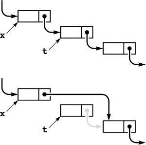
Figures 3.3 and 3.4 show the two fundamental operations that we perform on linked lists. We can delete any item from a linked list, to make it shrink by 1 in length; and we can insert an item into a linked list at any point, to make it grow by 1 in length. For simplicity, we assume in these figures that the lists are circular and never become empty. We will consider null links, dummy nodes, and empty lists in Section 3.4. As shown in the figures, insertion and deletion each require just two statements in C. To delete the node following node x, we use the statements
t = x->next; x->next = t->next;
To delete, or remove, the node following a given node x from a linked list, we set t to point to the node to be removed, then change x’s link to point to t->next. The pointer t can be used to refer to the removed node (to return it to a free list, for example). Although its link still points into the list, we generally do not use such a link after removing the node from the list, except perhaps to inform the system, via free, that its memory can be reclaimed.
Figure 3.3 Linked-list deletion
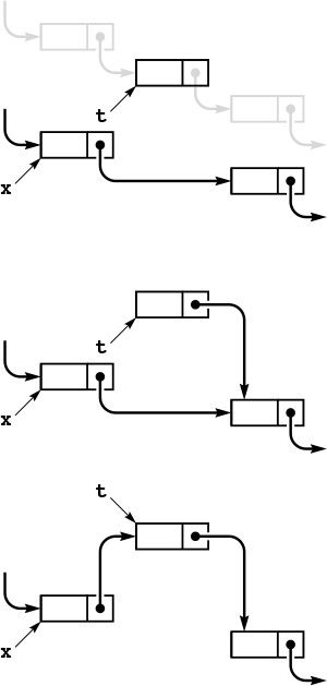
To insert a given node t into a linked list at a position following another given node x (top), we set t->next to x->next (center), then set x->next to t (bottom).
Figure 3.4 Linked-list insertion
or simply
x->next = x->next->next;
To insert node t into a list at a position following node x, we use the statements
t->next = x->next; x->next = t;
The simplicity of insertion and deletion is the raison d’etre of linked lists. The corresponding operations are unnatural and inconvenient in arrays, because they require moving all of the array’s contents following the affected item.
By contrast, linked lists are not well suited for the find the kth item (find an item given its index) operation that characterizes efficient access in arrays. In an array, we find the kth item simply by accessing a[k]; in a list, we have to traverse k links. Another operation that is unnatural on singly linked lists is “find the item before a given item.”
When we remove a node from a linked list using x->next = x->next->next, we may never be able to access it again. For small programs such as the examples we consider at first, this is no special concern, but we generally regard it as good programming practice to use the function free, which is the counterpart to malloc, for any node that we no longer wish to use. Specifically, the sequence of instructions
t = x->next; x->next = t->next; free(t);
not only removes t from our list but also informs the system that the memory it occupies may be used for some other purpose. We pay particular attention to free when we have large list objects, or large numbers of them, but we will ignore it until Section 3.5, so that we may focus on appreciating the benefits of linked structures.
We will see many examples of applications of these and other basic operations on linked lists in later chapters. Since the operations involve only a few statements, we often manipulate the lists directly rather than defining functions for inserting, deleting, and so forth. As an example, we consider next a program for solving the Josephus problem in the spirit of the sieve of Eratosthenes.
We imagine that N people have decided to elect a leader by arranging themselves in a circle and eliminating every Mth person around the circle, closing ranks as each person drops out. The problem is to find out which person will be the last one remaining (a mathematically inclined potential leader will figure out ahead of time which position in the circle to take). The identity of the elected leader is a function of N and M that we refer to as the Josephus function. More generally, we may wish to know the order in which the people are eliminated. For example, as shown in Figure 3.5, if N = 9 and M = 5, the people are eliminated in the order 5 1 7 4 3 6 9 2, and 8 is the leader chosen. Program 3.9 reads in N and M and prints out this ordering.
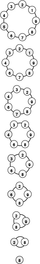
This diagram shows the result of a Josephus-style election, where the group stands in a circle, then counts around the circle, eliminating every fifth person and closing the circle.
Figure 3.5 Example of Josephus election
Program 3.9 uses a circular linked list to simulate the election process directly. First, we build the list for 1 to N: We build a circular list consisting of a single node for person 1, then insert the nodes for people 2 through N, in that order, following that node in the list, using the insertion code illustrated in Figure 3.4. Then, we proceed through the list, counting through M – 1 items, deleting the next one using the code illustrated in Figure 3.3, and continuing until only one node is left (which then points to itself).
The sieve of Eratosthenes and the Josephus problem clearly illustrate the distinction between using arrays and using linked lists to represent a sequentially organized collection of objects. Using a linked list instead of an array for the sieve of Eratosthenes would be costly because the algorithm’s efficiency depends on being able to access any array position quickly, and using an array instead of a linked list for the Josephus problem would be costly because the algorithm’s efficiency depends on the ability to delete items quickly. When we choose a data structure, we must be aware of the effects of that choice upon the efficiency of the algorithms that will process the data. This interplay between data structures and algorithms is at the heart of the design process and is a recurring theme throughout this book.
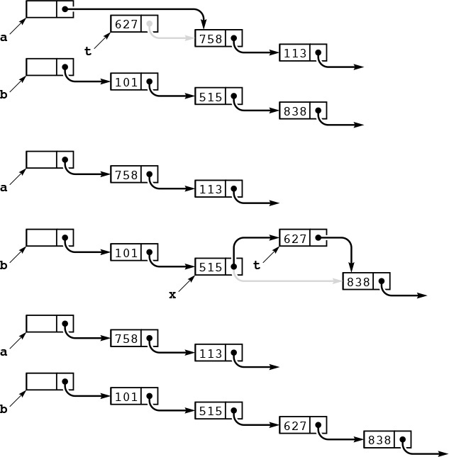
In C, pointers provide a direct and convenient concrete realization of the abstract concept of a linked list, but the essential value of the abstraction does not depend on any particular implementation. For example, Figure 3.6 shows how we could use arrays of integers to implement the linked list for the Josephus problem. That is, we can implement linked lists using array indices, instead of pointers. Linked lists are thus useful even in the simplest of programming environments. Linked lists were useful well before pointer constructs were available in high-level languages such as C. Even in modern systems, simple array-based implementations are sometimes convenient.

This sequence shows the linked list for the Josephus problem (see Figure 3.5), implemented with array indices instead of pointers. The index of the item following the item with index 0 in the list is next[0], and so forth. Initially (top three rows), the item for person i has index i-1, and we form a circular list by setting next[i] to i+1 for i from 0 to 8 and next[8] to 0. To simulate the Josephus-election process, we change the links (next array entries) but do not move the items. Each pair of lines shows the result of moving through the list four times with x = next[x], then deleting the fifth item (displayed at the left) by setting next[x] to next[next[x]].
Figure 3.6 Array representation of a linked list
Exercises
![]() 3.24 Write a function that returns the number of nodes on a circular list, given a pointer to one of the nodes on the list.
3.24 Write a function that returns the number of nodes on a circular list, given a pointer to one of the nodes on the list.
3.25 Write a code fragment that determines the number of nodes that are between the nodes referenced by two given pointers x and t to nodes on a circular list.
3.26 Write a code fragment that, given pointers x and t to two disjoint circular lists, inserts the list pointed to by t into the list pointed to by x, at the point following x.
![]() 3.27 Given pointers
3.27 Given pointers x and t to nodes on a circular list, write a code fragment that moves the node following t to the position following the node following x on the list.
3.28 When building the list, Program 3.9 sets twice as many link values as it needs to because it maintains a circular list after each node is inserted. Modify the program to build the circular list without doing this extra work.
3.29 Give the running time of Program 3.9, within a constant factor, as a function of M and N.
3.30 Use Program 3.9 to determine the value of the Josephus function for M = 2, 3, 5, 10, and N = 103, 104, 105, and 106.
3.31 Use Program 3.9 to plot the Josephus function versus N for M = 10 and N from 2 to 1000.
![]() 3.32 Redo the table in Figure 3.6, beginning with item
3.32 Redo the table in Figure 3.6, beginning with item i initially at position N-i in the array.
3.33 Develop a version of Program 3.9 that uses an array of indices to implement the linked list (see Figure 3.6).
3.4 Elementary List Processing
Linked lists bring us into a world of computing that is markedly different from that of arrays and structures. With arrays and structures, we save an item in memory and later refer to it by name (or by index) in much the same manner as we might put a piece of information in a file drawer or an address book; with linked lists, the manner in which we save information makes it more difficult to access but easier to rearrange. Working with data that are organized in linked lists is called list processing.
When we use arrays, we are susceptible to program bugs involving out-of-bounds array accesses. The most common bug that we encounter when using linked lists is a similar bug where we reference an undefined pointer. Another common mistake is to use a pointer that we have changed unknowingly. One reason that this problem arises is that we may have multiple pointers to the same node without necessarily realizing that that is the case. Program 3.9 avoids several such problems by using a circular list that is never empty, so that each link always refers to a well-defined node, and each link can also be interpreted as referring to the list.
Developing correct and efficient code for list-processing applications is an acquired programming skill that requires practice and patience to develop. In this section, we consider examples and exercises that will increase our comfort with working with list-processing code. We shall see numerous other examples throughout the book, because linked structures are at the heart of some of our most successful algorithms.
As mentioned in Section 3.3, we use a number of different conventions for the first and final pointers in a list. We consider some of them in this section, even though we adopt the policy of reserving the term linked list to describe the simplest situation.
Definition 3.3 A linked list is either a null link or a link to a node that contains an item and a link to a linked list.
This definition is more restrictive than Definition 3.2, but it corresponds more closely to the mental model that we have when we write list-processing code. Rather than exclude all the other various conventions by using only this definition, and rather than provide specific definitions corresponding to each convention, we let both stand, with the understanding that it will be clear from the context which type of linked list we are using.
One of the most common operations that we perform on lists is to traverse them: We scan through the items on the list sequentially, performing some operation on each. For example, if x is a pointer to the first node of a list, the final node has a null pointer, and visit is a function that takes an item as an argument, then we might write
for (t = x; t != NULL; t = t->next) visit(t->item);
to traverse the list. This loop (or its equivalent while form) is as ubiquitous in list-processing programs as is the corresponding
for (i = 0; i < N; i++)
in array-processing programs.
Program 3.10 is an implementation of a simple list-processing task, reversing the order of the nodes on a list. It takes a linked list as an argument, and returns a linked list comprising the same nodes, but with the order reversed. Figure 3.7 shows the change that the function makes for each node in its main loop. Such a diagram makes it easier for us to check each statement of the program to be sure that the code changes the links as intended, and programmers typically use these diagrams to understand the operation of list-processing implementations.
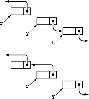
To reverse the order of a list, we maintain a pointer r to the portion of the list already processed, and a pointer y to the portion of the list not yet seen. This diagram shows how the pointers change for each node in the list. We save a pointer to the node following y in t, change y’s link to point to r, and then move r to y and y to t.
Figure 3.7 List reversal
Program 3.11 is an implementation of another list-processing task: rearranging the nodes of a list to put their items in sorted order. It generates N random integers, puts them into a list in the order that they were generated, rearranges the nodes to put their items in sorted order, and prints out the sorted sequence. As we discuss in Chapter 6, the expected running time of this program is proportional to N2, so the program is not useful for large N. Beyond this observation, we defer discussing the sort aspect of this program to Chapter 6, because we shall see a great many methods for sorting in Chapters 6 through 10. Our purpose now is to present the implementation as an example of a list-processing application.
The lists in Program 3.11 illustrate another commonly used convention: We maintain a dummy node called a head node at the beginning of each list. We ignore the item field in a list’s head node, but maintain its link as the pointer to the node containing the first item in the list. The program uses two lists: one to collect the random input in the first loop, and the other to collect the sorted output in the second loop. Figure 3.8 diagrams the changes that Program 3.11 makes during one iteration of its main loop. We take the next node off the input list, find where it belongs in the output list, and link it into position.
This diagram depicts one step in transforming an unordered linked list (pointed to by a) into an ordered one (pointed to by b), using insertion sort. We take the first node of the unordered list, keeping a pointer to it in t (top). Then, we search through b to find the first node x with x->next->item > t->item (or x->next = NULL), and insert t into the list following x (center). These operations reduce the length of a by one node, and increase the length of b by one node, keeping b in order (bottom). Iterating, we eventually exhaust a and have the nodes in order in b.
Figure 3.8 Linked-list sort
The primary reason to use the head node at the beginning becomes clear when we consider the process of adding the first node to the sorted list. This node is the one in the input list with the smallest item, and it could be anywhere on the list. We have three options:
• Duplicate the for loop that finds the smallest item and set up a one-node list in the same manner as in Program 3.9.
• Test whether the output list is empty every time that we wish to insert a node.
• Use a dummy head node whose link points to the first node on the list, as in the given implementation.
The first option is inelegant and requires extra code; the second is also inelegant and requires extra time.
The use of a head node does incur some cost (the extra node), and we can avoid the head node in many common applications. For example, we can also view Program 3.10 as having an input list (the original list) and an output list (the reversed list), but we do not need to use a head node in that program because all insertions into the output list are at the beginning. We shall see still other applications that are more simply coded when we use a dummy node, rather than a null link, at the tail of the list. There are no hard-and-fast rules about whether or not to use dummy nodes—the choice is a matter of style combined with an understanding of effects on performance. Good programmers enjoy the challenge of picking the convention that most simplifies the task at hand. We shall see several such tradeoffs throughout this book.
For reference, a number of options for linked-list conventions are laid out in Table 3.1; others are discussed in the exercises. In all the cases in Table 3.1, we use a pointer head to refer to the list, and we maintain a consistent stance that our program manages links to nodes, using the given code for various operations. Allocating and freeing memory for nodes and filling them with information is the same for all the conventions. Robust functions implementing the same operations would have extra code to check for error conditions. The purpose of the table is to expose similarities and differences among the various options.
This table gives implementations of basic list-processing operations with five commonly used conventions. This type of code is used in simple applications where the list-processing code is inline.
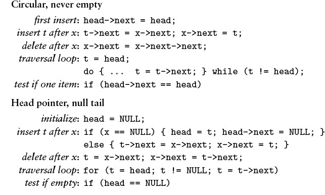
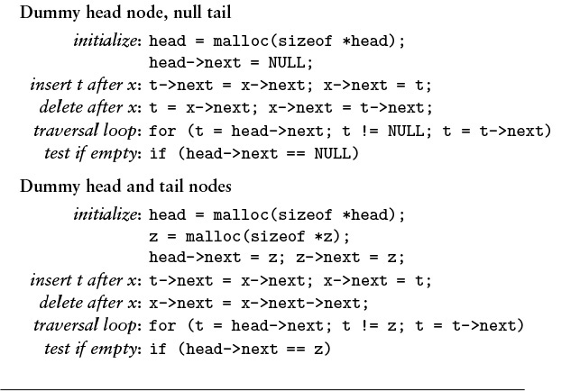
Table 3.1 Head and tail conventions in linked lists
Another important situation in which it is sometimes convenient to use head nodes occurs when we want to pass pointers to lists as arguments to functions that may modify the list, in the same way that we do for arrays. Using a head node allows the function to accept or return an empty list. If we do not have a head node, we need a mechanism for the function to inform the calling program when it leaves an empty list. One such mechanism—the one used for the function in Program 3.10—is to have list-processing functions take pointers to input lists as arguments and return pointers to output lists. With this convention, we do not need to use head nodes. Furthermore, it is well suited to recursive list processing, which we use extensively throughout the book (see Section 5.1).
Program 3.12 illustrates declarations for a set of black-box functions that implement the basic list operations, in case we choose not to repeat the code inline. Program 3.13 is our Josephus-election program (Program 3.9) recast as a client program that uses this interface. Identifying the important operations that we use in a computation and defining them in an interface gives us the flexibility to consider different concrete implementations of critical operations and to test their effectiveness. We consider one implementation for the operations defined in Program 3.12 in Section 3.5 (see Program 3.14), but we could also try other alternatives without changing Program 3.13 at all (see Exercise 3.52). This theme will recur throughout the book, and we will consider mechanisms to make it easier to develop such implementations in Chapter 4.
Some programmers prefer to encapsulate all operations on low-level data structures such as linked lists by defining functions for every low-level operation in interfaces like Program 3.12. Indeed, as we shall see in Chapter 4, the C class mechanism makes it easy to do so. However, that extra layer of abstraction sometimes masks the fact that just a few low-level operations are involved. In this book, when we are implementing higher-level interfaces, we usually write low-level operations on linked structures directly, to clearly expose the essential details of our algorithms and data structures. We shall see many examples in Chapter 4.
By adding more links, we can add the capability to move backward through a linked list. For example, we can support the operation “find the item before a given item” by using a doubly linked list in which we maintain two links for each node: one (prev) to the item before, and another (next) to the item after. With dummy nodes or a circular list, we can ensure that x, x->next->prev, and x->prev->next are the same for every node in a doubly linked list. Figures 3.9 and 3.10 show the basic link manipulations required to implement delete, insert after, and insert before, in a doubly linked list. Note that, for delete, we do not need extra information about the node before it (or the node after it) in the list, as we did for singly linked lists—that information is contained in the node itself.

In a doubly-linked list, a pointer to a node is sufficient information for us to be able to remove it, as diagrammed here. Given t, we set t->next->prev to t->prev (center) and t->prev->next to t->next (bottom).
Figure 3.9 Deletion in a doubly-linked list

To insert a node into a doubly-linked list, we need to set four pointers. We can insert a new node after a given node (diagrammed here) or before a given node. We insert a given node t after another given node x by setting t->next to x->next and x->next->prev to t(center), and then setting x->next to t and t->prev to x (bottom).
Figure 3.10 Insertion in a doubly-linked list
Indeed, the primary significance of doubly linked lists is that they allow us to delete a node when the only information that we have about that node is a link to it. Typical situations are when the link is passed as an argument in a function call, and when the node has other links and is also part of some other data structure. Providing this extra capability doubles the space needed for links in each node and doubles the number of link manipulations per basic operation, so doubly linked lists are not normally used unless specifically called for. We defer considering detailed implementations to a few specific situations where we have such a need—for example in Section 9.5.
We use linked lists throughout this book, first for basic ADT implementations (see Chapter 4), then as components in more complex data structures. Linked lists are many programmers’ first exposure to an abstract data structure that is under the programmers’ direct control. They represent an essential tool for our use in developing the high-level abstract data structures that we need for a host of important problems, as we shall see.
Exercises
![]() 3.34 Write a function that moves the largest item on a given list to be the final node on the list.
3.34 Write a function that moves the largest item on a given list to be the final node on the list.
3.35 Write a function that moves the smallest item on a given list to be the first node on the list.
3.36 Write a function that rearranges a linked list to put the nodes in even positions after the nodes in odd positions in the list, preserving the relative order of both the evens and the odds.
3.37 Implement a code fragment for a linked list that exchanges the positions of the nodes after the nodes referenced by two given links t and u.
![]() 3.38 Write a function that takes a link to a list as argument and returns a link to a copy of the list (a new list that contains the same items, in the same order).
3.38 Write a function that takes a link to a list as argument and returns a link to a copy of the list (a new list that contains the same items, in the same order).
3.39 Write a function that takes two arguments—a link to a list and a function that takes a link as argument—and removes all items on the given list for which the function returns a nonzero value.
3.40 Solve Exercise 3.39, but make copies of the nodes that pass the test and return a link to a list containing those nodes, in the order that they appear in the original list.
3.41 Implement a version of Program 3.10 that uses a head node.
3.42 Implement a version of Program 3.11 that does not use head nodes.
3.43 Implement a version of Program 3.9 that uses a head node.
3.44 Implement a function that exchanges two given nodes on a doubly linked list.
![]() 3.45 Give an entry for Table 3.1 for a list that is never empty, is referred to with a pointer to the first node, and for which the final node has a pointer to itself.
3.45 Give an entry for Table 3.1 for a list that is never empty, is referred to with a pointer to the first node, and for which the final node has a pointer to itself.
3.46 Give an entry for Table 3.1 for a circular list that has a dummy node, which serves as both head and tail.
3.5 Memory Allocation for Lists
An advantage of linked lists over arrays is that linked lists gracefully grow and shrink during their lifetime. In particular, their maximum size does not need to be known in advance. One important practical ramification of this observation is that we can have several data structures share the same space, without paying particular attention to their relative size at any time.
The crux of the matter is to consider how the system function malloc might be implemented. For example, when we delete a node from a list, it is one thing for us to rearrange the links so that the node is no longer hooked into the list, but what does the system do with the space that the node occupied? And how does the system recycle space such that it can always find space for a node when malloc is called and more space is needed? The mechanisms behind these questions provide another example of the utility of elementary list processing.
The system function free is the counterpart to malloc. When we are done using a chunk of allocated memory, we call free to inform the system that the chunk is available for later use. Dynamic memory allocation is the process of managing memory and responding to calls on malloc and free from client programs.
When we are calling malloc directly in applications such as Program 3.9 or Program 3.11, all the calls request memory blocks of the same size. This case is typical, and an alternate method of keeping track of memory available for allocation immediately suggests itself: Simply use a linked list! All nodes that are not on any list that is in use can be kept together on a single linked list. We refer to this list as the free list. When we need to allocate space for a node, we get it by deleting it from the free list; when we remove a node from any of our lists, we dispose of it by inserting it onto the free list.
Program 3.14 is an implementation of the interface defined in Program 3.12, including the memory-allocation functions. When compiled with Program 3.13, it produces the same result as the direct implementation with which we began in Program 3.9. Maintaining the free list for fixed-size nodes is a trivial task, given the basic operations for inserting nodes onto and deleting nodes from a list.
Figure 3.11 illustrates how the free list grows as nodes are freed, for Program 3.13. For simplicity, the figure assumes a linked-list implementation (no head node) based on array indices.

This version of Figure 3.6 shows the result of maintaining a free list with the nodes deleted from the circular list, with the index of first node on the free list given at the left. At the end of the process, the free list is a linked list containing all the items that were deleted. Following the links, starting at 1, we see the items in the order 2 9 6 3 4 7 1 5, which is the reverse of the order in which they were deleted.
Figure 3.11 Array representation of a linked list, with free list
Implementing a general-purpose memory allocator in a C environment is much more complex than is suggested by our simple examples, and the implementation of malloc in the standard library is certainly not as simple as is indicated by Program 3.14. One primary difference between the two is that malloc has to handle storage-allocation requests for nodes of varying sizes, ranging from tiny to huge. Several clever algorithms have been developed for this purpose. Another approach that is used by some modern systems is to relieve the user of the need to free nodes explicitly by using garbage-collection algorithms to remove automatically any nodes not referenced by any link. Several clever storage management algorithms have also been developed along these lines. We will not consider them in further detail because their performance characteristics are dependent on properties of specific systems and machines.
Programs that can take advantage of specialized knowledge about an application often are more efficient than general-purpose programs for the same task. Memory allocation is no exception to this maxim. An algorithm that has to handle storage requests of varying sizes cannot know that we are always going to be making requests for blocks of one fixed size, and therefore cannot take advantage of that fact. Paradoxically, another reason to avoid general-purpose library functions is that doing so makes programs more portable—we can protect ourselves against unexpected performance changes when the library changes or when we move to a different system. Many programmers have found that using a simple memory allocator like the one illustrated in Program 3.14 is an effective way to develop efficient and portable programs that use linked lists. This approach applies to a number of the algorithms that we will consider throughout this book, which make similar kinds of demands on the memory-management system.
Exercises
![]() 3.47 Write a program that frees (calls
3.47 Write a program that frees (calls free with a pointer to) all the nodes on a given linked list.
3.48 Write a program that frees the nodes in positions that are divisible by 5 in a linked list (the fifth, tenth, fifteenth, and so forth).
![]() 3.49 Write a program that frees the nodes in even positions in a linked list (the second, fourth, sixth, and so forth).
3.49 Write a program that frees the nodes in even positions in a linked list (the second, fourth, sixth, and so forth).
3.50 Implement the interface in Program 3.12 using malloc and free directly in allocNode and freeNode, respectively.
3.51 Run empirical studies comparing the running times of the memory-allocation functions in Program 3.14 with malloc and free (see Exercise 3.50) for Program 3.13 with M = 2 and N = 103, 104, 105, and 106.
3.52 Implement the interface in Program 3.12 using array indices (and no head node) rather than pointers, in such a way that Figure 3.11 is a trace of the operation of your program.
![]() 3.53 Suppose that you have a set of nodes with no null pointers (each node points to itself or to some other node in the set). Prove that you ultimately get into a cycle if you start at any given node and follow links.
3.53 Suppose that you have a set of nodes with no null pointers (each node points to itself or to some other node in the set). Prove that you ultimately get into a cycle if you start at any given node and follow links.
![]() 3.54 Under the conditions of Exercise 3.53, write a code fragment that, given a pointer to a node, finds the number of different nodes that it ultimately reaches by following links from that node, without modifying any nodes. Do not use more than a constant amount of extra memory space.
3.54 Under the conditions of Exercise 3.53, write a code fragment that, given a pointer to a node, finds the number of different nodes that it ultimately reaches by following links from that node, without modifying any nodes. Do not use more than a constant amount of extra memory space.
![]() 3.55 Under the conditions of Exercise 3.54, write a function that determines whether or not two given links, if followed, eventually end up on the same cycle.
3.55 Under the conditions of Exercise 3.54, write a function that determines whether or not two given links, if followed, eventually end up on the same cycle.
3.6 Strings
We use the term string to refer to a variable-length array of characters, defined by a starting point and by a string-termination character marking the end. Strings are valuable as low-level data structures, for two basic reasons. First, many computing applications involve processing textual data, which can be represented directly with strings. Second, many computer systems provide direct and efficient access to bytes of memory, which correspond directly to characters in strings. That is, in a great many situations, the string abstraction matches needs of the application to the capabilities of the machine.
The abstract notion of a sequence of characters ending with a string-termination character could be implemented in many ways. For example, we could use a linked list, although that choice would exact a cost of one pointer per character. The concrete array-based implementation that we consider in this section is the one that is built into C. We shall also examine other implementations in Chapter 4.
The difference between a string and an array of characters revolves around length. Both represent contiguous areas of memory, but the length of an array is set at the time that the array is created, whereas the length of a string may change during the execution of a program. This difference has interesting implications, which we shall explore shortly.
We need to reserve memory for a string, either at compile time, by declaring a fixed-length array of characters, or at execution time, by calling malloc. Once the array is allocated, we can fill it with characters, starting at the beginning, and ending with the string-termination character. Without a string-termination character, a string is no more or no less than an array of characters; with the string-termination character, we can work at a higher level of abstraction, and consider only the portion of the array from the beginning to the string-termination character to contain meaningful information. In C, the termination character is the one with value 0, also known as '�'.
For example, to find the length of a string, we count the number of characters between the beginning and the string-termination character. Table 3.2 gives simple operations that we commonly perform on strings. They all involve processing the strings by scanning through them from beginning to end. Many of these functions are available as library functions declared in <string.h>, although many programmers use slightly modified versions in inline code for simple applications. Robust functions implementing the same operations would have extra code to check for error conditions. We include the code here not just to highlight its simplicity, but also to expose its performance characteristics plainly.
This table gives implementations of basic string-processing operations, using two different C language primitives. The pointer approach leads to more compact code, but the indexed-array approach is a more natural way to express the algorithms and leads to code that is easier to understand. The pointer version of the concatenate operation is the same as the indexed array version, and the pointer version of prefixed compare is obtained from the normal compare in the same way as for the indexed array version and is omitted. The implementations all take time proportional to string lengths.
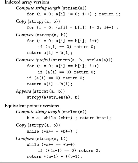
Table 3.2 Elementary string-processing operations
One of the most important operations that we perform on strings is the compare operation, which tells us which of two strings would appear first in the dictionary. For purposes of discussion, we assume an idealized dictionary (since the actual rules for strings that contain punctuation, uppercase and lowercase letters, numbers, and so forth are rather complex), and compare strings character-by-character, from beginning to end. This ordering is called lexicographic order. We also use the compare function to tell whether strings are equal—by convention, the compare function returns a negative number if the first argument string appears before the second in the dictionary, returns 0 if they are equal, and returns 1 if the first appears after the second in lexicographic order. It is critical to take note that doing equality testing is not the same as determining whether two string pointers are equal—if two string pointers are equal, then so are the referenced strings (they are the same string), but we also could have different string pointers that point to equal strings (identical sequences of characters). Numerous applications involve storing information as strings, then processing or accessing that information by comparing the strings, so the compare operation is a particularly critical one. We shall see a specific example in Section 3.7 and in numerous other places throughout the book.
Program 3.15 is an implementation of a simple string-processing task, which prints out the places where a short pattern string appears within a long text string. Several sophisticated algorithms have been developed for this task, but this simple one illustrates several of the conventions that we use when processing strings in C.
String processing provides a convincing example of the need to be knowledgeable about the performance of library functions. The problem is that a library function might take more time than we expect, intuitively. For example, determining the length of a string takes time proportional to the length of the string. Ignoring this fact can lead to severe performance problems. For example, after a quick look at the library, we might implement the pattern match in Program 3.15 as follows:
for (i = 0; i < strlen(a); i++)
if (strncmp(&a[i], p, strlen(p)) == 0)
printf("%d ", i);
Unfortunately, this code fragment takes time proportional to at least the square of the length of a, no matter what code is in the body of the loop, because it goes all the way through a to determine its length each time through the loop. This cost is considerable, even prohibitive: Running this program to check whether this book (which has more than 1 million characters) contains a certain word would require trillions of instructions. Problems such as this one are difficult to detect because the program might work fine when we are debugging it for small strings, but then slow down or even never finish when it goes into production. Moreover, we can avoid such problems only if we know about them!
This kind of error is called a performance bug, because the code can be verified to be correct, but it does not perform as efficiently as we (implicitly) expect. Before we can even begin the study of efficient algorithms, we must be certain to have eliminated performance bugs of this type. Although standard libraries have many virtues, we must be wary of the dangers of using them for simple functions of this kind.
One of the essential concepts that we return to time and again in this book is that different implementations of the same abstract notion can lead to widely different performance characteristics. For example, if we keep track of the length of the string, we can support a function that can return the length of a string in constant time, but for which other operations run more slowly. One implementation might be appropriate for one application; another implementation might be appropriate for another application.
Library functions, all too often, cannot guarantee to provide the best performance for all applications. Even if (as in the case of strlen) the performance of a library function is well documented, we have no assurance that some future implementation might not involve performance changes that will have adverse effects on our programs. This issue is critical in the design of algorithms and data structures, and thus is one that we must always bear in mind. We shall discuss other examples and further ramifications in Chapter 4.
Strings are actually pointers to chars. In some cases, this realization can lead to compact code for string-processing functions. For example, to copy one string to another, we could write
while (*a++ = *b++) ;
instead of
for (i = 0; a[i] != 0; i++) a[i] = b[i];
or the third option given in Table 3.2. These two ways of referring to strings are equivalent, but may lead to code with different performance properties on different machines. We generally use the array version for clarity and the pointer version for economy, reserving detailed study of which is best for particular pieces of frequently executed code in particular applications.
Memory allocation for strings is more difficult than for linked lists because strings vary in size. Indeed, a fully general mechanism to reserve space for strings is neither more nor less than the system-provided malloc and free functions. As mentioned in Section 3.6, various algorithms have been developed for this problem, whose performance characteristics are system and machine dependent. Often, memory allocation is a less severe problem when we are working with strings than it might first appear, because we work with pointers to the strings, rather that with the characters themselves. Indeed, we do not normally assume in C code that all strings sit in individually allocated chunks of memory. We tend to assume that each string sits in memory of indeterminate allocation, just big enough for the string and its termination character. We must be very careful to ensure adequate allocation when we are performing operations that build or lengthen strings. As an example, we shall consider a program that reads strings and manipulates them in Section 3.7.
Exercises
![]() 3.56 Write a program that takes a string as argument, and that prints out a table giving, for each character that occurs in the string, the character and its frequency of occurrence.
3.56 Write a program that takes a string as argument, and that prints out a table giving, for each character that occurs in the string, the character and its frequency of occurrence.
![]() 3.57 Write a program that checks whether a given string is a palindrome (reads the same backward or forward), ignoring blanks. For example, your program should report success for the string
3.57 Write a program that checks whether a given string is a palindrome (reads the same backward or forward), ignoring blanks. For example, your program should report success for the string if i had a hifi.
3.58 Suppose that memory for strings is individually allocated. Write versions of strcpy and strcat that allocate memory and return a pointer to the new string for the result.
3.59 Write a program that takes a string as argument and reads a sequence of words (sequences of characters separated by blank space) from standard input, printing out those that appear as substrings somewhere in the argument string.
3.60 Write a program that replaces substrings of more than one blank in a given string by exactly one blank.
3.61 Implement a pointer version of Program 3.15.
![]() 3.62 Write an efficient program that finds the length of the longest sequence of blanks in a given string, examining as few characters in the string as possible. Hint: Your program should become faster as the length of the sequence of blanks increases.
3.62 Write an efficient program that finds the length of the longest sequence of blanks in a given string, examining as few characters in the string as possible. Hint: Your program should become faster as the length of the sequence of blanks increases.
3.7 Compound Data Structures
Arrays, linked lists, and strings all provide simple ways to structure data sequentially. They provide a first level of abstraction that we can use to group objects in ways amenable to processing the objects efficiently. Having settled on these abstractions, we can use them in a hierarchical fashion to build up more complex structures. We can contemplate arrays of arrays, arrays of lists, arrays of strings, and so forth. In this section, we consider examples of such structures.
In the same way that one-dimensional arrays correspond to vectors, two-dimensional arrays, with two indices, correspond to matrices, and are widely used in mathematical computations. For example, we might use the following code to multiply two matrices a and b, leaving the result in a third matrix c.
for (i = 0; i < N; i++)
for (j = 0; j < N; j++)
for (k = 0, c[i][j] = 0.0; k < N; k++)
c[i][j] += a[i][k]*b[k][j];
We frequently encounter mathematical computations that are naturally expressed in terms of multidimensional arrays.
Beyond mathematical applications, a familiar way to structure information is to use a table of numbers organized into rows and columns. A table of students’ grades in a course might have one row for each student, and one column for each assignment. In C, such a table would be represented as a two-dimensional array with one index for the row and one for the column. If we were to have 100 students and 10 assignments, we would write grades[100][10] to declare the array, and then refer to the ith student’s grade on the jth assignment as grade[i][j]. To compute the average grade on an assignment, we sum together the elements in a column and divide by the number of rows; to compute a particular student’s average grade in the course, we sum together the elements in a row and divide by the number of columns, and so forth. Two-dimensional arrays are widely used in applications of this type. On a computer, it is often convenient and straightforward to use more than two dimensions: An instructor might use a third index to keep student-grade tables for a sequence of years.
Two-dimensional arrays are a notational convenience, as the numbers are ultimately stored in the computer memory, which is essentially a one-dimensional array. In many programming environments, two-dimensional arrays are stored in row-major order in a one-dimensional array: In an array a[M][N], the first N positions would be occupied by the first row (elements a[0][0] through a[0][N-1]), the second N positions by the second row (elements a[1][0] through a[1][N-1]), and so forth. With row-major order, the final line in the matrix-multiplication code in the beginning of this section is precisely equivalent to
The same scheme generalizes to provide a facility for arrays with more dimensions. In C, multidimensional arrays may be implemented in a more general manner: we can define them to be compound data structures (arrays of arrays). This provides the flexibility, for example, to have an array of arrays that differ in size.
We saw a method in Program 3.6 for dynamic allocation of arrays that allows us to use our programs for varying problem sizes without recompiling them, and would like to have a similar method for multidimensional arrays. How do we allocate memory for multidimensional arrays whose size we do not know at compile time? That is, we want to be able to refer to an array element such as a[i][j] in a program, but cannot declare it as int a[M][N] (for example) because we do not know the values of M and N. For row-major order, a statement like
int* a = malloc(M*N*sizeof(int));
would be an effective way to allocate an M-by-N array of integers, but this solution will not work in all C environments, because not all implementations use row-major order. Program 3.16 gives a solution for two-dimensional arrays, based on their definition as arrays of arrays.
Program 3.17 illustrates the use of a similar compound structure: an array of strings. At first blush, since our abstract notion of a string is an array of characters, we might represent arrays of strings as arrays of arrays. However, the concrete representation that we use for a string in C is a pointer to the beginning of an array of characters, so an array of strings can also be an array of pointers. As illustrated in Figure 3.12, we then can get the effect of rearranging strings simply by rearranging the pointers in the array. Program 3.17 uses the qsort library function—implementing such functions is the subject of Chapters 6 through 9 in general and of Chapter 7 in particular. This example illustrates a typical scenario for processing strings: we read the characters themselves into a huge one-dimensional array, save pointers to individual strings (delimiting them with string-termination characters), then manipulate the pointers.

When processing strings, we normally work with pointers into a buffer that contains the strings (top), because the pointers are easier to manipulate than the strings themselves, which vary in length. For example, the result of a sort is to rearrange the pointers such that accessing them in order gives the strings in alphabetical (lexicographic) order.
Figure 3.12 String sort
We have already encountered another use of arrays of strings: the argv array that is used to pass argument strings to main in C programs. The system stores in a string buffer the command line typed by the user and passes to main a pointer to an array of pointers to strings in that buffer. We use conversion functions to calculate numbers corresponding to some arguments; we use other arguments as strings, directly.
We can build compound data structures exclusively with links, as well. Figure 3.13 shows an example of a multilist, where nodes have multiple link fields and belong to independently maintained linked lists. In algorithm design, we often use more than one link to build up complex data structures, but in such a way that they are used to allow us to process them efficiently. For example, a doubly linked list is a multilist that satisfies the constraint that x->l->r and x->r->l are both equal to x. We shall examine a much more important data structure with two links per node in Chapter 5.
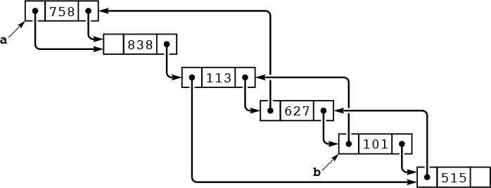
We can link together nodes with two link fields in two independent lists, one using one link field, the other using the other link field. Here, the right link field links together nodes in one order (for example, this order could be the order in which the nodes were created) and the left link field links together nodes in a different order (for example, in this case, sorted order, perhaps the result of insertion sort using the left link field only). Following right links from a, we visit the nodes in the order created; following left links from b, we visit the nodes in sorted order.
Figure 3.13 A multilist
If a multidimensional matrix is sparse (relatively few of the entries are nonzero), then we might use a multilist rather than a multidimensional array to represent it. We could use one node for each value in the matrix and one link for each dimension, with the link pointing to the next item in that dimension. This arrangement reduces the storage required from the product of the maximum indices in the dimensions to be proportional to the number of nonzero entries, but increases the time required for many algorithms, because they have to traverse links to access individual elements.
To see more examples of compound data structures and to highlight the distinction between indexed and linked data structures, we next consider data structures for representing graphs. A graph is a fundamental combinatorial object that is defined simply as a set of objects (called vertices) and a set of connections among the vertices (called edges). We have already encountered graphs, in the connectivity problem of Chapter 1.
We assume that a graph with V vertices and E edges is defined by a set of E pairs of integers between 0 and V-1. That is, we assume that the vertices are labeled with the integers 0, 1, ..., V-1, and that the edges are specified as pairs of vertices. As in Chapter 1 we take the pair i-j as defining a connection between i and j and thus having the same meaning as the pair j-i. Graphs that comprise such edges are called undirected graphs. We shall consider other types of graphs in Part 7.
One straightforward method for representing a graph is to use a two-dimensional array, called an adjacency matrix. With an adjacency matrix, we can determine immediately whether or not there is an edge from vertex i to vertex j, just by checking whether row i and column j of the matrix is nonzero. For the undirected graphs that we are considering, if there is an entry in row i and column j, then there also must be an entry in row j and column i, so the matrix is symmetric. Figure 3.14 shows an example of an adjacency matrix for an undirected graph; Program 3.18 shows how we can create an adjacency matrix, given a sequence of edges as input.
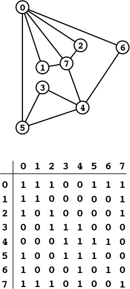
A graph is a set of vertices and a set of edges connecting the vertices. For simplicity, we assign indices (nonnegative integers, consecutively, starting at 0) to the vertices. An adjacency matrix is a two-dimensional array where we represent a graph by putting a 1 bit in row i and column j if and only if there is an edge from vertex i to vertex j. The array is symmetric about the diagonal. By convention, we assign 1 bits on the diagonal (each vertex is connected to itself). For example, the sixth row (and the sixth column) says that vertex 6 is connected to vertices 0, 4, and 6.
Figure 3.14 Graph with adjacency matrix representation
Another straightforward method for representing a graph is to use an array of linked lists, called adjacency lists. We keep a linked list for each vertex, with a node for each vertex connected to that vertex. For the undirected graphs that we are considering, if there is a node for j in i’s list, then there must be a node for i in j’s list. Figure 3.15 shows an example of the adjacency-lists representation of an undirected graph; Program 3.19 shows how we can create an adjacency-lists representation of a graph, given a sequence of edges as input.
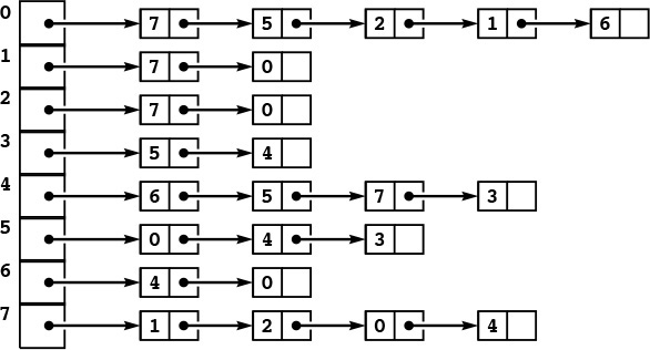
This representation of the graph in Figure 3.14 uses an array of lists. The space required is proportional to the number of nodes plus the number of edges. To find the indices of the vertices connected to a given vertex i, we look at the ith position in an array, which contains a pointer to a linked list containing one node for each vertex connected to i.
Figure 3.15 Adjacency-lists representation of a graph
Both graph representations are arrays of simpler data structures—one for each vertex describing the edges incident on that vertex. For an adjacency matrix, the simpler data structure is implemented as an indexed array; for an adjacency list, it is implemented as a linked list.
Thus, we face straightforward space tradeoffs when we represent a graph. The adjacency matrix uses space proportional to V2; the adjacency lists use space proportional to V + E. If there are few edges (such a graph is said to be sparse), then the adjacency-lists representation uses far less space; if most pairs of vertices are connected by edges (such a graph is said to be dense), the adjacency-matrix representation might be preferable, because it involves no links. Some algorithms will be more efficient with the adjacency-matrix representation, because it allows the question “is there an edge between vertex i and vertex j?” to be answered in constant time; other algorithms will be more efficient with the adjacency-lists representation, because it allows us to process all the edges in a graph in time proportional to V + E, rather than to V2. We see a specific example of this tradeoff in Section 5.8.
Both the adjacency-matrix and the adjacency-lists graph representations can be extended straightforwardly to handle other types of graphs (see, for example, Exercise 3.71). They serve as the basis for most of the graph-processing algorithms that we shall consider in Part 7.
To conclude this chapter, we consider an example that shows the use of compound data structures to provide an efficient solution to the simple geometric problem that we considered in Section 3.2. Given d, we want to know how many pairs from a set of N points in the unit square can be connected by a straight line of length less than d.
Program 3.20 uses a two-dimensional array of linked lists to improve the running time of Program 3.8 by a factor of about 1/d2 when N is sufficiently large. It divides the unit square up into a grid of equal-sized smaller squares. Then, for each square, it builds a linked list of all the points that fall into that square. The two-dimensional array provides the capability to access immediately the set of points close to a given point; the linked lists provide the flexibility to store the points where they may fall without our having to know ahead of time how many points fall into each grid square.
The space used by Program 3.20 is proportional to 1/d2 + N, but the running time is O(d2N2), which is a substantial improvement over the brute-force algorithm of Program 3.8 for small d. For example, with N = 106 and d = 0.001, we can solve the problem in time and space that is effectively linear, whereas the brute-force algorithm would require a prohibitive amount of time. We can use this data structure as the basis for solving many other geometric problems, as well. For example, combined with a union-find algorithm from Chapter 1, it gives a near-linear algorithm for determining whether a set of N random points in the plane can be connected together with lines of length d—a fundamental problem of interest in networking and circuit design.
As suggested by the examples that we have seen in this section, there is no end to the level of complexity that we can build up from the basic abstract constructs that we can use to structure data of differing types into objects and sequence the objects into compound objects, either implicitly or with explicit links. These examples still leave us one step away from full generality in structuring data, as we shall see in Chapter 5. Before taking that step, however, we shall consider the important abstract data structures that we can build with linked lists and arrays—basic tools that will help us in developing the next level of generality.
Exercises
3.63 Write a version of Program 3.16 that handles three-dimensional arrays.
3.64 Modify Program 3.17 to process input strings individually (allocate memory for each string after reading it from the input). You can assume that all strings have less than 100 characters.
3.65 Write a program to fill in a two-dimensional array of 0–1 values by setting a[i][j] to 1 if the greatest common divisor of i and j is 1, and to 0 otherwise.
3.66 Use Program 3.20 in conjunction with Program 1.4 to develop an efficient program that can determine whether a set of N points can be connected with edges of length less than d.
3.67 Write a program to convert a sparse matrix from a two-dimensional array to a multilist with nodes for only nonzero values.
![]() 3.68 Implement matrix multiplication for matrices represented with multilists.
3.68 Implement matrix multiplication for matrices represented with multilists.
![]() 3.69 Show the adjacency matrix that is built by Program 3.18 given the input pairs
3.69 Show the adjacency matrix that is built by Program 3.18 given the input pairs 0-2, 1-4, 2-5, 3-6, 0-4, 6-0, and 1-3.
![]() 3.70 Show the adjacency lists that are built by Program 3.19 given the input pairs
3.70 Show the adjacency lists that are built by Program 3.19 given the input pairs 0-2, 1-4, 2-5, 3-6, 0-4, 6-0, and 1-3.
![]() 3.71 A directed graph is one where vertex connections have orientations: edges go from one vertex to another. Do Exercises 3.69 and 3.70 under the assumption that the input pairs represent a directed graph, with
3.71 A directed graph is one where vertex connections have orientations: edges go from one vertex to another. Do Exercises 3.69 and 3.70 under the assumption that the input pairs represent a directed graph, with i-j signifying that there is an edge from i to j. Also, draw the graph, using arrows to indicate edge orientations.
3.72 Modify Program 3.18 to take the number of vertices as a command-line argument, then dynamically allocate the adjacency matrix.
3.73 Modify Program 3.19 to take the number of vertices as a command-line argument, then dynamically allocate the array of lists.
![]() 3.74 Write a function that uses the adjacency matrix of a graph to calculate, given vertices a and b, the number of vertices c with the property that there is an edge from a to c and from c to b.
3.74 Write a function that uses the adjacency matrix of a graph to calculate, given vertices a and b, the number of vertices c with the property that there is an edge from a to c and from c to b.
![]() 3.75 Answer Exercise 3.74, but use adjacency lists.
3.75 Answer Exercise 3.74, but use adjacency lists.