
Chapter 5
Structured Representations
STRUCTURE IN MENTAL REPRESENTATIONS
What is the scope of a representational element, for example, a representation for the concept robin? If the representation contains the feature red, does this feature describe the whole bird or just part of it? The extent or domain of a representational element is its scope. Every representation I have discussed so far contains some assumptions about the scope of its representational elements.
For the spatial and featural representations discussed in chapters 2 and 3, the scope of the representational elements was implicit. In mental space models, concepts were represented as points in a multidimensional space. In models derived from multidimensional scaling techniques, the dimensions of the space were assumed to have some meaning. Each point had a value along each dimension of the space, and each dimension value was restricted in scope to the point in space corresponding to a particular concept. If a psychological dimension represents the color of an object, the point for robin occupies a region corresponding to red on the color dimension. This representation of red has some ambiguity, because the dimension value is associated with the point representing the concept as a whole, and it is difficult to represent that only some part of the robin is red.
In featural models, concepts were represented by sets of features, and each feature described only the concept denoted by the feature set. A given feature might be part of a substitutive dimension, so that having one value of a feature precluded the object’s having other values along the same dimension. In the case of a representation for the concept robin, each feature in a set applies to the whole concept, and to represent that the whole robin is red, the feature red is added to the feature set. It is difficult to represent that a feature is true of only a part of an object. Features themselves have no means for restricting their scope (e.g., restricting the scope of red to the breast of the robin). For this reason, representational schemes have made the scope of representational elements explicit.
Semantic networks, like those discussed in chapter 4, are one type of representation in which the scope of representational elements was made explicit. Because each node is connected to other nodes via labeled links, the scope of the relation described by a link is restricted to the nodes that it connects. Figure 5.1 shows a piece of a network representing the fact that a robin has a red breast. Here the connection between robin and breast makes it clear that the breast is a part of the robin. Another connection between breast and red makes it clear that the breast is red, although other parts of the robin may be other colors. Thus, the semantic network contains explicit information about the scope of representational elements.
In chapter 4, I focused on processes in network models that spread activation across links. In these models, labels were important primarily for interpreting paths between nodes found when activation tags intersected. The processes discussed in chapter 4 were not concerned with the scope of the representational elements. In chapters 5 through 7, I discuss structured representations in which the processes acting over these representations are sensitive to the scope of the representational elements. In this chapter, I introduce terminology for describing structured representations and describe some of their basic characteristics. Then, I present processing assumptions that have been used in conjunction with structured representations in psychology and logic. In chapter 6, I extend these basic principles by examining the use of structure in models of perception and imagery. In chapter 7, I describe the use of structured representations in conceptual representations, notably scripts and schemas, to complete the introductory tour of structured representations.
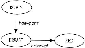
FIG. 5.1. Simple semantic network demonstrating that the scope of the links is determined by the nodes to which they are connected.
THE BASICS OF STRUCTURED REPRESENTATIONS
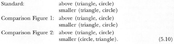
Determining the scope of representational elements is a critical aspect of the notion of representation. Because the scope of most elements seems intuitively obvious, it is easy to underestimate the importance of this aspect of representation. Figure 5.2 shows a pair of geometric configurations that are clearly different. One pair is a striped square above a shaded circle, and the other is a striped circle above a shaded square. Nonetheless, if I listed a set of features that describe these configurations without worrying about the scope of the representational elements, then I may find that the same set of features can describe both configurations. Figure 5.3A shows sets of features that describe both configurations in Figure 5.2. I have conveniently divided this feature list into sections to make it clear which features belong to which objects in Figure 5.2. An actual feature list would not have this structure, and one would know only that the same set of features describes both configurations.
In a structured representation, one creates the scope of representational elements by allowing elements in a representation to take arguments that restrict their scope. For example, I can describe the square in the left configuration in Figure 5.2 with the statement:
![]()
In Example 5.1, striped, is a representational element, and square is its argument; the scope of the property striped is restricted to describing a square. This representation is a predicate because it represents something true (or false) in the represented world. Predicates with one argument (like the one in Example 5.1) are attributes, which typically represent de-scriptive properties of their argument.
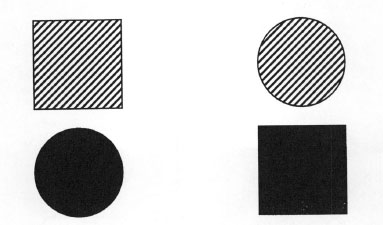
FIG. 5.2. Geometric configurations.
Another important type of predicate is the relation, which is a predicate with two or more arguments. Relations are used to represent relationships that hold between elements in a represented world. For example, the predicate:
![]()
represents the spatial relationship between the square and the circle in the left configuration in Figure 5.2. The same representation in graph form appears in Figure 5.3C, which shows a graph of structured representations for the two configurations in Figure 5.2. In this figure, predicates are connected to their arguments by links. Although arrows can be used to show the directions of the links, they are usually omitted for the sake of clarity.1
Finally, not all statements in a structured representation are predicates: Not all statements are things whose truth in the represented world can be determined. Statements evaluated for something other than their truth are called functions. For example, the size of an object in the represented world can be described by the function:
![]()
In this example, size (circle) is a function because it cannot be determined to correspond to a true or false state of the represented world. Instead, size (circle) has some value in the represented world.
One can treat this function as a representation and consider it a placeholder for the size of the circle if, for example, one is making an analogy between one object that is larger than another and a sound that is louder than a second (Gentner, Rattermann, Markman, & Kotovsky, 1995). In this case, one can represent the difference in size as:
![]()
and the difference in loudness as:
![]()
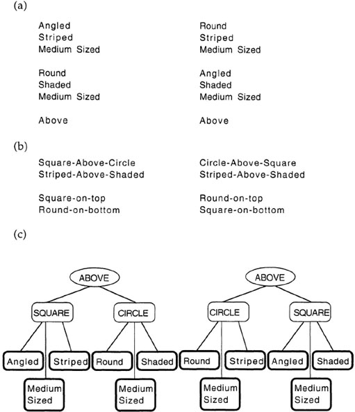
FIG. 5.3. A: Features representing the geometric configurations in Figure 5.2. B: Configural features that can be added to the feature representation. C: Graph of structured representations of the geometric configurations.
This representation highlights the fact that the size in Example 5.4 is similar to the loudness in Example 5.5. The specific value of the size of the object or the loudness of the sound does not matter, only the fact that the object has a size and the sound has a loudness.
In other cases, one might want to evaluate the function. Presumably, the function size (circle) is associated with a process for determining the size of the circle, so one can find its value (e.g., medium-sized). The evaluation of functions is an important part of computer programming; in languages like LISP, functions can be used both as representational elements (as in Examples 5.4 and 5.5) and as processes. In this way, the distinction between representation and process gets blurred.
Constants and Variables
The predicates described so far have arguments that represent specific elements in the represented world. These elements are often called constants, a term borrowed from logic. Constants are used when the elements described by a predicate are known, but it is also possible to represent situations in which the particular elements that are arguments to a predicate are unknown. In this case, one uses variables in the representation; a variable is a placeholder whose value is unknown, like a box that is eventually filled with a value. For example, I can represent the general fact that something is above something else by using this statement:
![]()
In this statement, ?x and ?y are variables whose values are unknown. A statement consisting of predicates whose arguments are constants (or variables that are bound to some value) is called a proposition because it denotes a possible state of affairs in the represented world. In structured representations, the meaning of a proposition is compositional and is determined by the meanings of the proposition’s constituent elements.
Variables in a structured representation can be free to take on any value or can be restricted to certain types of values. In computer programming, many languages use type restrictions on variables. In PASCAL, for example, a variable may be restricted to take on integer values, real number values, or even strings of characters. Type restrictions on variables have also been incorporated into structured representations, often as a low-cost way to make sure that something being represented is likely to be interpretable. For example, if a system tries to create a representation in which the predicate marry (?x, ?y) is applied to inanimate objects, one may need to investigate another type of meaning (perhaps a metaphorical meaning). Type restrictions, sometimes called case roles, are also common in linguistic models (e.g., Fillmore, 1968).
Type restrictions on variables ease the specification of processes in a domain. If predicates are guaranteed to have arguments of a particular type, rules formulated to reason about these predicates can make assumptions about the predicates’ arguments. In chapter 9, I discuss qualitative process (QP) theory (Forbus, 1984), which was designed to reason about physical systems. In this system, the predicates that describe quantities require their arguments to be quantities. Because of this type restriction, all rules about quantities can assume that the predicates supposed to describe quantities actually do describe quantities. Thus, one need not have each rule check the arguments of the predicates to find out what they are. There are, however, potential costs to this use of type restrictions. First, the set of types must be known in advance so that the case roles can be created. If new case roles are added after some knowledge has already been entered into the system, old knowledge may not obey new case-role restrictions. Second, it is necessary to specify the processes checking the arguments to ensure that they obey the case roles when representations are constructed. Thus, as discussed previously, adding a new complexity to a representation (like type restrictions) requires new machinery to process it.
Number and Type of Arguments
Structured representations are not limited in the number of their arguments. Any element can be identified by the number of arguments that it takes. Elements with no arguments are called constants if the value is known and variables if it is unknown. Elements that take a single argument are called unary elements; those that take two arguments are called binary elements. In general, the arity of an element refers to the number of arguments that it takes.
In the examples discussed so far, the arguments to predicates and functions have all been constants or variables. A predicate whose arguments are all constants or variables is called a first-order predicate. Predicates may also have arguments that are other statements with arguments. The sentence “Mary kissed John causingjohn to hug Mary” can be represented as:
![]()
In this case, both arguments to the relation cause (?x, ?y) are themselves relations. The cause (?x, ?y) relation in Example 5.7 is a second-order predicate because it contains at least one argument that is a first-order predicate. More generally, the order of a predicate is one greater than the order of the highest order element that is an argument to that predicate. As discussed next, higher order relations are often used to represent important conceptual relations like causal relations.
Why Use Structured Representations?
Structured representations make explicit the relations between elements in a situation, and they allow complex representations to be constructed through the combination of simpler elements. The simple configurations of shapes in Figure 5.2 illustrate this issue; the sets of features in Figure 5.3A represent these configurations with lists of features. As discussed earlier, the feature lists describing the left and right configurations actually contain the same set of features. If the representations of these configurations were truly the same, the configurations would be perceived as identical. Because they are not so perceived, something must be done to the representation to allow the configurations to be differentiated.
One extension to the feature lists in Figure 5.3A includes an additional set of configural features, like those in Figure 5.3B. These features encode large-scale configural aspects of the scenes like the fact that there is a square on top of a circle in the left configurations, and a circle on top of a square in the right configuration. This clearly solves part of the problem. Now the representation has explicit information about the relationships between the shapes, and the configurations are no longer seen as identical. Configural features are themselves features, which either match a feature in a second representation or do not. There are no partially matching features. The absence of partial matches is a problem because one can adopt a very large set of possible configural features. Any pair of attributes can potentially enter into a configural feature for every binary relation that holds for the configuration: square-above-circle, round-above-angled, striped-above-shaded, or even square-above-shaded or shaded-and-medium-sized-above-round. In addition, configural features can specify only part of an existing relation like square-on-top or round-on-bottom. These configural features are useful for finding similarities between configurations with only a partial match. The problem with configural features is that the number of possible configural features grows exponentially as the number of elements and relations to be represented grows (e.g., Foss & Harwood, 1975).
Structured representations provide an alternative to feature lists for representing situations like the one in Figure 5.2. Because representational elements contain connections to their arguments, the same element can be reused with different arguments to represent different situations. Because graphs contain the same information as the formulaic notation used in Examples 5.1 through 5.7, the representation in Figure 5.3C can be written as:
above (square, circle)
angled (square)
striped (square)
medium-sized (square)
round (circle)
shaded (circle)
medium-sized (circle).
(5.8)
With the structured representation for representing this situation, similar configurations can use similar representational elements with different sets of arguments. The circle above the square in the right configuration can be represented by using the same relation as the square above the circle with the arguments reversed. In this way, there is a partial match between these representations, and the attributes of the shapes are explicitly attached to the elements they describe. Thus, in the left configuration, it is not just that something is shaded, but rather that a circle is shaded. The common relation leads to the perception of differences in the arguments to the relation. I expand this point next.
Evidence for the Importance of Structure
In the previous section, I suggest that structured representations are more efficient than are feature lists, but as discussed in chapter 4, people are not always maximally efficient. Thus, it remains to be demonstrated that structured representations make predictions that are consistent with people’s behavior. Indeed, research in perception suggests that people sometimes err when perceiving objects in a manner suggesting they may not bind attributes to the right objects. In a classic set of studies, Treisman and Schmidt (1982) found illusory conjunctions of features. An illusory conjunction occurs when people report seeing an object with a particular conjunction of features when, in fact, the pair of features was not initially part of the same object. For example, they may report seeing a blue N when they had actually been shown a blue S and a red N. In one study, researchers quickly flashed to the subjects a display with two numbers and some colored letters and asked them to report the digits and whatever else they saw in the scene. Under these conditions, people reported a number of illusory conjunctions. Indeed, on some trials subjects actually reported seeing colored numbers, even though they were always shown the numbers in black. These data suggest that colors and shapes are initially processed separately and bound together only later in processing. During initial processing, a perceptual feature need not have a scope that corresponds to the scope of the property in the represented world. It may require visual attention to ensure that the perceptual properties of objects are bound together properly.
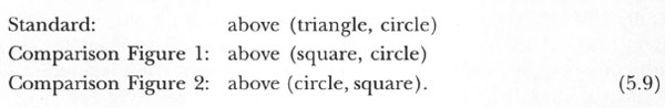
In normal circumstances, of course, people do not observe these illusory conjunctions, and research on similarity has supported the assumption that cognitive representations are structured. In a simple study by Markman, Gentner, and Wisniewski (1998), we gave people a forced-choice task. We showed them a standard and two comparison figures and asked them to select the comparison figure that was most similar to the standard. The stimuli and results appear in Figure 5.4. We presented subjects with eight forced-choice triads in a random order. In Figure 5.4, the comparison figures in the middle column were preferred to those in the right column by a majority of subjects (at least 8 out of 10 in this study, p <.05 by sign test).
The first triad (top row) demonstrates that people find configurations with similar objects in them to be more similar than are configurations with dissimilar objects. In the next two triads (2a, 2b), people prefer configurations with the same relation to those without the same relation, even when the objects that play similar relational roles are different. In Triad 2a, there is a triangle on top and a circle on the bottom in the standard and a circle on top and a triangle on the bottom in the preferred comparison figure. In Triad 2b, the shapes in the comparison figures are different from those in the standard altogether. So far, these results are equally compatible with either featural or structured representations. Both featural representations and structured representations simply have to assume that having features describing similar objects make a pair of configurations similar, and features describing relations (without considering relational roles) also make a pair of configurations similar.
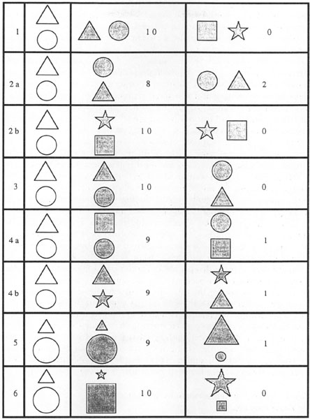
FIG. 5.4. Stimuli from a study of similarity of geometric configurations. Ten subjects reported which comparison figure in the right-most two columns was most similar to the standard in the left-most column. The numbers are the number of subjects selecting each alternative. The favored alternative always appears in the middle column.
With Triad 3, the situation grows more complex: Similar objects in the same relational roles make a pair more similar than similar objects in different relational roles. To account for this pattern, a featural view needs to have global configural features like above-triangle-circle, but such global configural features are insufficient, as demonstrated by Triads 4a and 4b. Here, having only one similar object playing the same relational role in the target and the comparison figure makes the configurations more similar than having no similar objects playing the same relational roles. In addition to global configural features, a featural view must assume that there are other configural features like circle-on-the-bottom and triangle-on-the-top to account for people’s choices in these triads.
Triad 5 demonstrates that people also prefer consistency across a number of different relations in a scene. In the standard, the triangle is above the circle and is also smaller than the circle. Subjects preferred a comparison figure that preserves both these relational commonalities over one that preserves only one. If a featural view were to represent this new relation, a new (and large) set of configural features must be added to handle the new relation. Finally, Triad 6 demonstrates that this preference for relational consistency holds even when none of the actual objects in the standard and the comparison figure is similar. Thus, people can process multiple relational similarities in the absence of any similarity between the objects.
How Do Structural Representations Account for These Findings?
To this point, the study illustrated in Figure 5.4 suggests only that featural representations provide an unwieldy and unsatisfying explanation for the pattern of data observed. How does a structured representation account for these data? In order to understand similarity in the case of structured representations, it is necessary to pay more careful attention to how structured representations are processed. In chapter 3, I described A. Tversky’s (1977) contrast model, which modeled similarity comparisons as the comparison of feature lists. In this model, feature representations were just sets; the elementary set operation of intersection could be used to find the common features of a pair, and the operation of set difference could be used to find the distinctive features of a pair.
With structured representations, the situation grows more complex: Now, the comparison process must be sensitive to the argument structure of the representations. Models of similarity assuming structured representations have adopted a structural alignment framework (Gentner & Markman, 1997). Structural alignment is a process derived from studies of how people understand analogies (Gentner, 1983, 1989; Gentner & Markman, 1997; Hesse, 1966; Holyoak & Thagard, 1989, 1995; Keane, Ledgeway, & Duff, 1994; Markman & Gentner, 1993a, 1993b; Medin, Goldstone, & Gentner, 1993). This research is strongly related to Gentner’s (1983, 1989) structure-mapping theory. The structural alignment process is substantially more complex than is the simple set operations that were sufficient to compare features lists, because this process must be sensitive to the connections among relations and attributes and their bindings.
In the structural alignment process, people seek a match between structured representations that is rooted in semantic similarity and maintains structural consistency. The use of semantic similarity implies that at least some matching elements must have identical names, an assumption ensuring that any perceived similarity is rooted in at least one semantic commonality between representations. For example, if the two representations in Figure 5.3C are compared, the above (?x, ?y) relations can be matched because they have the same name. Any match must also be structurally consistent, where structural consistency involves two constraints: parallel connectivity and one-to-one mapping. Parallel connectivity states that if two elements in a representation are placed in correspondence, their arguments must also be placed in correspondence. In Figure 5.3C, placing the above (?x, ?y) relations in correspondence causes the square in the left representation to be placed in correspondence with the circle in the right representation because both are the first arguments to the above (?x, ?y) relation (i.e., both are on top). Likewise, the circle in the left representation can be placed in correspondence with the square in the right representation because both are the second arguments to the above relation (i.e., both are on the bottom). One-to-one mapping requires that each element in one representation be placed in correspondence with at most one element in the other representation. Thus, placing the square in the left representation with the circle in the right representation because both are on the top precludes also placing the square in the left representation in correspondence with the square in the right representation because both are angled. To see both the similarity of the square to the circle because each plays a common relational role and the similarity of the square to the square because both are angled, the structural alignment process must calculate two distinct mappings, each of which has a unique set of object correspondences. This process has been embodied in different computational models that take as input structured representations and yield a set of correspondences between the domains (Falkenhainer, Forbus, & Gentner, 1989; Holyoak & Thagard, 1989; Hummel & Holyoak, 1997; Keane et al., 1994).
The structural alignment process allows a straightforward explanation of the results of the study in Figure 5.4. For example, the configurations in Triad 4a can be represented2 as:
With these representations, both comparison figures have a common relation with the standard, but parallel connectivity requires that the arguments of the relations also be placed in correspondence. The second argument of Comparison Figure 1 in Figure 5.4 matches that of the standard; the second argument of Comparison Figure 2 does not. Hence, Comparison Figure 1 has an extra commonality that Comparison Figure 2 lacks.
One can give similar explanations for all the triads in Figure 5.4. Readers may draw a set of representations to verify that the structural alignment view of similarity predicts judging Comparison Figure 1 more similar to the standard than is Comparison Figure 2 for all the triads. One additional example, however, is helpful. Triad 5 can be represented as:
In this case, when Comparison Figure 1 is compared to the standard, both the above (?x, ?y) relation and the smaller (?x, ?y) relation can be matched, because each of these relations maps the triangle to the triangle and the circle to the circle. In contrast, when Comparison Figure 2 is compared to the standard, either the above (?x, ?y) relation or the smaller (?x, ?y) relation but not both can be placed in correspondence because matching these two relations involves different object correspondences. Matching the above (?x, ?y) relations places the triangle in the standard in correspondence with the triangle in the comparison figure and the circle in the standard with the circle in the comparison figure. In contrast, matching the smaller (?x, ?y) relation places the triangle in the standard in correspondence with the circle in the comparison figure and the circle in the standard in correspondence with the triangle in the comparison figure. By one-to-one mapping, both sets of correspondences cannot coexist. Thus, the match between the first comparison figure and the standard is preferred.
Structure and Determination of Commonalities and Differences
The structural alignment view of similarity has implications beyond simply accounting for people’s ability to make comparisons involving relations. In particular, making use of the connection between elements and their arguments allows for the possibility that commonalities and differences are related. In chapter 3, I described the contrast model and stated that the sets of common and distinctive features are assumed to be independent. In contrast to this assumption, the structural alignment view assumes that commonalities and differences are deeply connected.
Figure 5.5 shows another set of geometric configurations along with graphs of structured representations that can describe these configurations. If these configurations are compared, they may look similar because there is something above something else in each of them. On this view, the commonalities of the configurations include something above something else in each; striped, medium-sized things on top; and checked, medium-sized things on the bottom. Because the scenes look similar on the basis of the common above (?x, ?y) relation, the circle in the left configuration is placed in correspondence with the square in the right configuration. Likewise, the square in the left configuration is placed in correspondence with the circle in the right configuration. The elements placed in correspondence (e.g., the circle and square on top) are perceived as different because they were placed in correspondence by virtue of a commonality. Thus, they are alignable differences. In contrast, the triangle in the left configuration has no correspondence at all with anything in the right configuration. Elements in one representation with no correspondence at all with elements in the other (like the triangle) are called nonalignable differences.
The distinction between alignable and nonalignable differences may be easier to see by considering an alternative form of structured representation called conceptual frames (Barsalou, 1992; Lenat & Guha, 1990; Minsky, 1981). As shown in Figure 5.6, a conceptual frame highlights the dimensional structure of the item represented. In its simplest form, a frame consists of a number of binary relations between a concept, a dimension along which the concept varies (a slot or an attribute), and a value that fills the dimension for that concept (a filler or value). Although the frame is just a collection of these binary relations, this aspect of frames is obscured by the fact that frames are typically written like the one in Figure 5.6, in which the concept heads the list and the slots and their fillers are listed below it (Hayes, 1979).
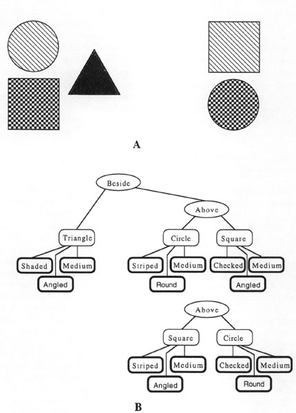
FIG. 5.5. A: Simple configurations of objects; B: simple relational structure describing the configurations. From “Comparisons,” by A. B. Markman and D. Gentner, 1996, Memory and Cognition, 24(2), p. 236. Copyright © 1996 by The Psychonomic Society. Reprinted with permission.
In a comparison of conceptual frames, an alignable difference can be thought of as a matching slot between two concepts with a mismatching value. In contrast, a nonalignable difference can be thought of as a slot of one concept with no corresponding slot in the other. In Figure 5.6, the concept robin has a slot eats that is filled with what it eats. If a robin is compared to a chair, the concept chair probably would not have an eats slot, because the action of eating does not make sense for chairs. Because there is no equivalent slot for eats in the concept chair, the fact that robins eat worms would probably be seen as a nonalignable difference in a comparison of robin and chair.
The distinction between alignable and nonalignable differences has been explored in numerous studies (Gentner & Markman, 1994; Markman & Gentner, 1993a, 1996, 1997; Markman & Wisniewski, 1997). In one set of studies, researchers asked subjects to list the commonalities or differences of pairs of similar words (e.g., yacht/sailboat) and pairs of dissimilar words (e.g., shopping mall/traffic light). Not surprisingly, people listed more commonalities for pairs of similar words than for pairs of dissimilar words, but they also listed more alignable differences for pairs of similar words than for pairs of dissimilar words. A person might say that a yacht and a sailboat differ because sailboats have sails and yachts have motors, that yachts are more expensive than sailboats, and that yachts often travel longer than do sailboats. There are few obvious alignable differences for shopping mall and traffic light, although one might say that a traffic light has red, amber, and green lights, and a shopping mall has primarily white lights.
FIG. 5.6. Sample conceptual frame.
In contrast to the pattern of listed alignable differences, people listed more nonalignable differences for pairs of dissimilar words than for pairs of similar words. In general, researchers using this commonality- and difference-listing methodology have found a positive correlation between the number of listed commonalities and the number of listed differences across a wide range of stimuli, including pairs of concrete nouns, pairs of abstract nouns, pairs of verbs, and pairs of pictures. For example, one might say that a yacht has deck chairs on it, but a sailboat does not. In contrast, almost any property of a shopping mall has no correspondence with a traffic light and vice versa. One could say that a shopping mall has stores and a traffic light does not, that a shopping mall has places to eat and a traffic light does not, that a traffic light controls what cars do and a shopping mall does not.
A second important aspect of the distinction between alignable and nonalignable differences is that alignable differences are a more focal output of the comparison process than are nonalignable differences. A. Tversky’s work on the contrast model suggested that commonalities are generally more important to the perceived similarity of a pair than are differences. Structural alignment also assumes that differences related to commonalities (the alignable differences) are more important to perceived similarity than are differences not related to commonalities (the nonalignable differences). In support of this view, Markman and Gentner (1996) found that people’s similarity ratings were affected more by variations in alignable differences than by variations in nonalignable differences.
Other cognitive tasks that involve comparisons also seem to favor alignable over nonalignable differences. In one study, researchers asked people to choose between pairs of video games that were described by different properties (Markman & Medin, 1995). After making a selection, the subjects justified their choices. The justifications were more likely to include properties that were alignable differences between the games than to include properties that were nonalignable differences. Investigators obtained this finding whether the properties were perceived to be important or unimportant elements of the options (Lindemann & Markman, 1996). Thus, people may systematically ignore information they believe to be important when the information is nonalignable with what they know about other options.
OTHER USES OF STRUCTURED REPRESENTATIONS
Representations with bindings between elements have been a part of many cognitive models both in psychology and computer science. Because these representations are generally more complex than are feature lists or spatial representations, the processing assumptions of the models are likewise more complex. In this section, I first discuss production system models, which have been used as general architectures for understanding cognitive skills. Then, I turn to the use of structured representations in logic. This work is particularly important, because, although it is probably implausible as the basis of a psychological model, it does introduce the idea that a representation may not refer to a specific individual, but may delimit a class of individuals. Because much research in artificial intelligence has used logic, it is worth being familiar with some basic principles of representation in logic.
Production Systems
Production systems are general computational models of cognitive processing that assume cognition involves the acquisition and execution of rules governing behavior (J. R. Anderson, 1983a, 1993; Newell, 1990). In this section, I discuss only the general principles underlying production systems. Proposals about production systems differ in the specific mechanisms they use to model cognitive processes. Readers interested in the application of production systems to psychology should refer to excellent introductions of the ACT-R system (J. R. Anderson, 1993) and the SOAR system (Newell, 1990), which are two of the best worked-out production system models of psychological processing.
The basic element of a production system is the production rule, which consists of a condition and an action. The condition is a state of affairs that must exist for the rule to be applicable. The action is the thing to be done if the rule is applied (rule application is often called rule firing). The entire condition of a rule must be satisfied for a production to be eligible to fire. If only some parts of the condition are satisfied by the current state of the world, the rule may not be applied. For example, a simple production rule may be:
This example is oversimplified because elements like “you are at the street corner” must be defined explicitly enough for the presence of this state to be detected. This rule clearly applies only if all of its conditions are met. If you are at a street corner and there are cars coming, it is dangerous to cross the street. If you are at a street corner and there are no cars coming but you do not want to cross the street, then you should not cross.
Often, many possible rules can be applied in a given situation. A production system must decide which rule to apply in situations in which more than one rule is applicable. Different production system models use different strategies for making this choice: perhaps the rule that was fired most recently or the most specific rule applicable (i.e., the one with the most parts to its condition).
Production system models use structured representations. Their representation of the world typically consists of relations and attributes. The condition part of a production rule is made up of relations and attributes that must be active in working memory for the rule to fire. The action part of a production rule specifies changes to be made in working memory (e.g., setting new goals, adding new facts) and actions to be taken in the world (e.g., instructions to effectors that operate on the world). J. R. Anderson’s (1993) ACT-R system doing simple addition will be used to illustrate the operation of a production system. J. R. Anderson provided a complete description of this system as well as a computer implementation of it. The basic elements of the production system for doing arithmetic are shown in Figure 5.7.
To define a production system for any domain, there must be a knowledge base and a set of rules for acting in the domain. In the case of addition, there must be facts that define what an addition problem is, facts that define what numbers are, and facts that define the known facts about addition and goals. For example, in Figure 5.7, there is a definition of the structure of a column in a production system, as well as an example of a specific column that may appear in an addition problem. There are also definitions of addition facts (like 6 + 3) and definitions of values of specific numbers. All these facts are written in a frame notation. As discussed earlier, frames can be thought of as binary relations connecting the concept to the value via a relation defined by the slot. Thus, memory in this production system corresponds to several different binary relations.
Acting on these facts are a number of production rules. The system can carry out only actions that have rules defining them. To process a column, the system must have the goal to answer a problem and must focus on a particular object in the problem, in this case a particular column in the problem. The column is defined as an array on the left side of Figure 5.7. The notation ?num means that the value from the fact is substituted in the variable defined by ?variable name. In production systems, a variable can take on different values each time a rule is applied. As discussed previously, variables are typically contrasted with constants, whose values remain fixed with each application of a rule. Once the variable has been bound, its value can be referred to as = variable name. Thus, the condition of the PROCESS COLUMN production in the right column first must have the goal to solve an addition problem and must focus on a column with numbers in its first two rows and a blank answer row. It must also have an addition fact in memory corresponding to the numbers in the first two rows of the column. The sum of the column (obtained from the known addition fact) is then bound into the new variable sum. If these conditions hold, the action may be carried out. In this case, a new goal is established to write the answer into the bottom row, where the answer to be written is the sum derived from the addition fact. The sum itself cannotjust be written into the column because it may involve a carry, and separate procedures for dealing with sums greater and less than nine must be established.
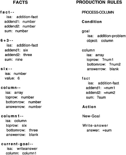
FIG. 5.7. Facts and production rules from J. R. Anderson’s example of simple addition.
Obviously, the production that processes a single column is only one element in a system doing simple addition. There must be productions that begin by finding the right-most column, productions that shift attention to the next left-most column after the current column has been processed, productions that write the answer, and productions that know how to deal with carries. There also must be facts supporting the productions, like the facts for all 100 of the two-addend one-digit addition facts. Although this amount of information seems great, it is consistent with the observation that students in grade school spend a lot of time learning basic arithmetic facts so that they can solve complex arithmetic problems.
There are three main things to take away from this simple production system. First, the representations have to be structured. Because it is important to be able to represent which numbers are in which column, the scope of each representational element must be known. This problem cannot be solved with only a list of features. Second, much information goes into the ability to solve even a simple problem. Doing arithmetic involves a large number of basic facts and procedures. Production systems leave out other important aspects of addition such as the ability to visually recognize the numbers. People who do arithmetic often make marks on paper, such as small numbers to indicate carries, to facilitate the task. This interaction of perceptual and motor skills in solving cognitive problems is often not addressed in production system models, because most such models are not connected to sensors (i.e., organs that sense the world) and effectors (i.e., mechanisms that influence the world). Instead, they assume that there are sensors providing input in a format amenable to the production system and effectors taking instructions in the form generated by the production system. (I return to this issue in chap. 10.)
Production systems use the concept of variables, which at first have no defined value and only acquired values during processing. Variables allow the same rule to be applied to a variety of situations by simply allowing a value to be bound to each variable. For example, in the PROCESS COLUMN production in Figure 5.7, the variables allow the production to be applied to a column with any numbers in it and to take whatever sum is known to result from the combination of any pair of addends. Variables go beyond the power of the representational systems described in previous chapters. In featural and spatial representations, for example, one can represent the properties of a particular individual or class of individuals but not a hypothetical individual. As discussed in the next section, variables are crucial for allowing a system to represent hypothetical individuals and groups, such as the quantifiers all, some, and none.
In chapter 4, I noted that production systems can be combined with spreading activation models of memory to explain the effects of working memory on cognitive processing. This combination can occur by assuming that each fact in memory (like those on the left side of Figure 5.7) has some level of activation associated with it. The probability of any given production’s firing is proportional to the activation associated with the elements that appear in the condition of the rule. Thus, if all facts in the condition of a rule are strongly activated, the probability of the rule’s firing is very high. If there are elements in the condition of the rule that are not at all activated, the rule is unlikely to fire. In this way, a semantic network with spreading activation can explain aspects of processing that involve the automatic spread of activation through memory, whereas a production system can explain rule-governed and goal-directed processes.
Quantification in Logic
Structured representations are an important part of systems of logical reasoning. Logic representations have been studied extensively; if a statement can be represented as a logical sentence, rules of logic can be carried out to predict what happens next or to infer properties of objects. A person may assert:
![]()
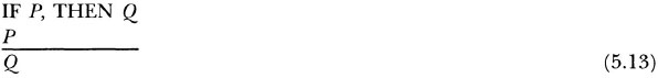
If the person later learns that it is raining, he or she can immediately infer that it is cloudy, because of the logical inference schema modus ponens:
In addition, if a person knows that it is not cloudy, he or she can infer that it is not raining by using the logical inference schema modus tollens:
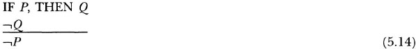
where ¬Q means “not (Q).” The beauty of these deductive inference schemas is that if the premises are true (e.g., if it is really the case that the rule IF P, THEN Q holds and it is really true that P) the conclusion must be true (it must really be the case that Q). The truth of the conclusion is guaranteed by the form (i.e., the syntax) of the rule without reference to its content. With any rule of the form If P, then Q, for any facts P and Q, the schemas modus ponens and modus tollens are valid. The many deductive reasoning schemas and proof procedures that have been developed have been the basis of cognitive models. Logic-based models have been applied most often in artificial intelligence (AI) (McCarthy, 1968), but some logic-based psychological models have been developed as well (Braine, Reiser, & Rumain, 1984; Rips, 1994).
The desire to have techniques yielding knowledge bases that are logically consistent and that contain facts known to be true is certainly a reasonable motivation for pursuing research on representations for doing logic. There is an additional aspect of logic systems, however, that allows them to represent an individual whose identity is not important. The representational systems described in previous chapters have allowed representations of individual items. The represented items may be specific objects in the represented world, such as a neighbor’s pet cat. The items may also be categories of objects in the represented world, such as cats in general. In a spatial representation, each item was represented by a point in a multidimensional space; in a featural representation, each item was represented by a set of features.
Consider, however, the lyric from the Eagles’ song “Heartache Tonight,” “Somebody wants to hurt someone.” Who wants to hurt someone? Whom do they want to hurt? Listeners cannot know, and in a sense, do not care. The statement “Somebody wants to hurt someone” does not name an unknown generic individual; it merely posits the existence of somebody who fits the characteristic of wanting to hurt someone. With a later lyric in the same song, “Nobody wants to go home now,” a similar issue arises. Listeners do not want to have to name each individual present at the event in question and somehow represent that the individual does not want to go home. Rather, they want to make a generic statement that applies to everybody.
Logic makes a provision for statements of this kind through the use of quantifiers. In particular, two quantifiers are important: the existential quantifier ∃, which means “There Exists,” and the universal quantifier ∀, which means “For All.” When used to define the values of variables, these quantifiers allow them to refer to individuals. The meaning of a statement like “Somebody wants to hurt someone” then reduces to a quantified statement that describes the characteristics of individuals for which the statement is true. For example, I can represent this sentence as
![]()
This statement means that there exist two people (bound to the variables ?x and ?y) such that both are people, and x wants to hurt y.3 Who x and y bind to in this example is unimportant. If this sentence is true, it is enough to know that there are people who exist and who satisfy these constraints. A similar case can be made for “Nobody wants to go home now,” which I can represent using the existential quantifier as:
![]()
This sentence can be read as meaning that it is not the case that there is some person who wants to go home now.4 On the surface, this reading somewhat differs from “Nobody wants to go home now,” but it works out to the same thing.
This section does not begin to do justice to the elegance and complexity of first-order logic. There are many excellent introductions to first-order logic and the role of quantification in logic representations for those who want more information (e.g., Barwise & Etchemendy, 1993a). In the context of this chapter, however, the main aspect of logical representations that is of interest is the use of quantified variables. By using variables and constraining them with the existential and universal quantifiers, one can represent individuals so that the identity of the individual is less important than are the constraints that the individual must satisfy. The ability to do such quantification is important in a variety of situations, such as language comprehension. Mechanisms for doing this quantification are important representational tools for many tasks, even those for which formal logical systems may be inappropriate.
HIGHER ORDER RELATIONAL STRUCTURE
Structured representations gain some of their power from the ability to create increasingly complex representations of a situation by embedding relations in other relations and thereby creating higher order relational structures. These higher order structures can encode important psychological elements like causal relations and implications. In Example 5.15, I created a representation of a quantified statement that somebody wants to hurt someone and used the arbitrary predicate wants-to-hurt (?x, ?y) for this representation. One would probably not want to use this predicate in a representation, because it is likely to apply in only a small range of circumstances. Unfortunately, to encode this situation using only first-order relations is quite difficult (see footnote 4 for one possibility).
The problem with representing “Somebody wants to hurt someone” arises from the fact that there is a state of the world that is desired by someone. Desire is a propositional attitude (Dennett, 1987; J. A. Fodor, 1981), a psychological state that someone can have about some proposition. Other propositional attitudes are believe and know. These prepositional attitudes are difficult to represent using only first-order predicates, because the object of the propositional attitude is itself a relation. They become much easier to represent with higher order relations. Example 5.15 can be recast with higher order relations as:
![]()
This representation contains two higher order relations. The first, which corresponds to the propositional attitude of desire, takes two arguments: the person who desires the state of affairs and the desired state of affairs. The second higher order relation expands the notion of what it means to hurt someone. In particular, it is a causal relation in which the antecedent to the causal relation is that some person carries out some action and the consequent to the relation is that person y is hurt.5
In this example, the higher order relations encode important facts about the domain. Relations like propositional attitudes and causal relations are central and often bind into a single structure many facts known about a domain. Higher order relations bring coherence to a domain; without them, there are only lists of facts, and it may be difficult to determine what information is important. Thus, being able to represent things as higher order relations may provide one avenue for helping the cognitive system to focus attention on important information. The idea that higher order relational structures lend coherence to, and are the source of important information in, a domain is called the systematicity principle (Gentner, 1983, 1989).6
TABLE 5.1
Summary of Stories Used to Test the Role of Systematicity in Analogy
Note. Key facts are shown in boldface; matching causal information is shown in italics.
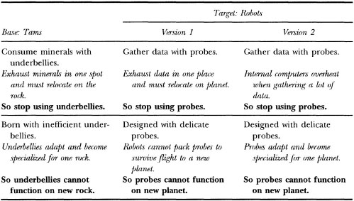
Systematicity has been shown to influence the way people process analogy and similarity comparisons. Earlier I discussed evidence that people’s perception of similarity is influenced by structure in concept representations. Related work has focused on the importance of systematicity in comparison. In one study, Clement and Gentner (1991) told people stories that had causal relations in them, one pair of which is illustrated in Table 5.1. The base story tells of organisms (the Tams) that feed off minerals from rocks by using their underbellies. The story had two central facts, as shown in the table. First, when the Tams deplete the minerals in one spot, they must relocate to a second rock and then stop using their underbellies. Second, their underbellies become specialized to a particular kind of rock and cannot function on another kind. After reading this first story, researchers gave subjects one version of a second, analogous story about robots on a distant planet (e.g., Version 1 in Table 5.1), in which the robots gather data with probes. In the story, neither of the causal consequents (shown in boldface in Table 5.1) was given. One causal antecedent was analogous to an antecedent in the Tam story (e.g., the data in one location were exhausted), and one was not (e.g., the robots cannot pack the probes to survive a flight). After reading the stories, workers asked subjects to make one new prediction about the robots in view of the similarity with the Tams. People were far more likely to infer the consequent with the matching causal antecedent (e.g., that the robots stop using the probes) than to infer the consequent without a matching causal antecedent (e.g., that the probes cannot function on a new planet). The reverse pattern was observed when participants were given Version 2 of the robot story. This finding is an instance of systematicity: People carried over information from the first story to the second only when the new information was governed by a higher order relation that was connected to matching facts between the stories. This finding has been replicated in other studies of analogical inference (Markman, 1997; Spellman & Holyoak, 1996).
Systematicity is not restricted to analogical inference; it also seems to be true of similarity-based inductive inferences. Lassaline (1996) asked participants to rate the strength of several inductive inferences. In these inductive inferences, some facts were known about one object, and some other facts were known about a second object. For example, a subject might know that facts A, B, and C were true of the first object and facts A and D were true of the second object. Then, investigators asked subjects to rate the likelihood that another property of the first object (B) was also true of the second. In some cases, a causal relation connected the property to be inferred to a property shared by the two objects (e.g., participants were told that A causes B). In other cases, there was no such causal relation. People judged that inferences in which the causal relation was present were stronger than were inferences in which the causal relation was not present. That is, when there was a causal relation in the first object linking properties A and B, the inference that the second object had property B was deemed stronger than when there was no causal relation linking A and B in the first object. These results suggest that systematicity helps focus people on information that is important in a situation.
Although there is evidence that systematicity constrains cognitive processing, particularly in analogy and inference, other evidence has also suggested that people do not have unlimited ability to embed one relation in another. In particular, researchers have looked at both children’s and adults’ ability to represent propositional attitudes (especially belief). Studies with children have focused on their ability to solve false belief tasks (Perner, 1991; Wellman, 1990). Typical false belief studies with children have involved describing situations to children in which a person is in a room and an object (e.g., a candy bar) is placed in some location (e.g., a cupboard). Then, the children are told that the person leaves the room, and while the person is out of the room, the object is moved to a new location (e.g., a bread box). Researchers asked children where the person will look for the candy bar when he or she returns to the room. When children are about 3 years old, they respond that the person will look in the location to which the object was moved (e.g., in the bread box), even though the person had left the room before the candy bar was moved and could not know where it was. Thus, children of this age seem to have trouble separating what they know (e.g., that the candy bar is in the bread box) from what the character knows (e.g., that the candy bar is in the cupboard).
By the time children are about 5 years old (and on into adulthood), they respond that the person will look in the original location (e.g., the cupboard). There has been some controversy over the age at which children respond correctly. The results in these tasks are influenced by the way the question is asked, but it clearly takes some time for children to develop the ability to represent other people’s beliefs. This task requires that a child represent a propositional attitude explicitly:
![]()
even though the proposition that the character believes does not correspond to what the child knows to be true about the world.
If studies of this type were the only ones to bear on this issue, children’s representational abilities would seem to gradually develop sophistication like their abilities to represent relations among propositions.7 Research with adults, however, has suggested that people are not always accurate in tasks involving reasoning about other people’s beliefs (e.g., Keysar, 1994; Keysar & Bly, 1995). Keysar (1994) presented adults with passages describing a situation in which a woman recommends a restaurant to a man because she has just enjoyed a wonderful meal there. When the man goes to the restaurant, the food and service are terrible. The next day, he leaves her a note saying, “The restaurant was marvelous, just marvelous.” The researchers asked the subjects how the woman will interpret this note. Many people suggested that the woman would interpret it as sarcasm, even though she had no way of knowing the man had a bad meal there. The finding that even adults seem to have some difficulty keeping track of other people’s beliefs qualifies the simple developmental story about propositional attitudes. The ability to represent other people’s beliefs does not seem to develop to the point that flawless performance on false belief tasks ensues. Rather, the ability to keep track of other people’s beliefs requires some effort, particularly in the complex settings studied by Keysar. Without the motivation to expend this effort, people may not choose to represent others’ beliefs. At present, there is no good theory about why representing propositional attitudes requires effort.
STRUCTURED REPRESENTATIONS AND CONNECTIONISM
Structured representations seem incompatible with connectionist models like those discussed in chapter 2. As described there, simple distributed connectionist models essentially use spatial representations. New vectors are compared to old vectors by using the dot product, which determines the degree of one vector that projects on another (in a high-dimensional space). In general, spatial representations like those in connectionist models using the dot product as the main measure of similarity are inappropriate as models of the structural comparisons described in this chapter, because they do not consider the relations between predicates and their arguments. Researchers have, however, developed more complex connectionist architectures that implement structured representations.
To create a structured representation in a connectionist system, the model must be extended in time or space to accommodate bindings between elements. Investigators have used both types of extensions. An example of a model’s extension in space is Smolensky’s tensor product model (Halford, 1992; Smolensky, 1990). In a tensor product model, elements to be bound together are first represented as N-dimensional vectors, in which each element is given a unique pattern of activity. To bind together two vectors, their outer product is taken. (The outer product was discussed in chap. 2, when I described the storage of associations in a simple network.) The outer product of two N-dimensional vectors yields an N × N matrix. To create the tensor product vector, the columns of the matrix are concatenated sequentially. The first column forms the first N rows of the vector, the next column forms the next N rows, and so on. Thus, a tensor product vector has N2 units. For example, to represent the proposition red (ball), I take the vector for red:
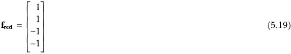
and the vector for ball:
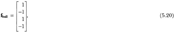
then take their outer product to yield:
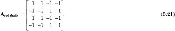
Then, I simply take the columns of this matrix and extend them out to form a vector as follows:
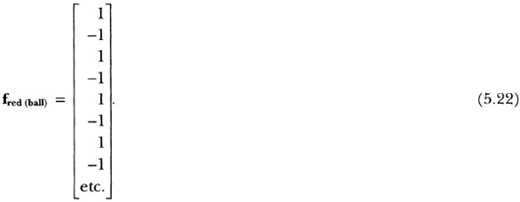
The tensor product can be used as a vector in another association. Because the tensor product is essentially an outer product, if the vector for red is presented to the system again, the vector for ball can be extracted by multiplying this outer product matrix with the vector (as discussed in chap. 2). Thus, the tensor product extends the dimensionality of the representation to bind pairs of vectors together.
It is important to consider what makes pairs of tensor product vectors similar to each other. It would be interesting if comparing pairs of tensor product vectors (by taking their dot product) would yield patterns of similarity similar to those obtained in studies of structural similarity, like those described earlier in this chapter. Holyoak and Hummel (in press) provided a formal account of the similarity of pairs of tensor product vectors. They demonstrated that the dot product of a pair of tensor product vectors is simply the product of the dot products of the constituent vectors of the tensor product vector. That is, the dot product (dp) of a tensor product vector that binds a pair of vectors a and b to a second vector that binds together the vectors c and d is:
![]()
Thus, if corresponding constituents of a pair of tensor product vectors are extremely dissimilar (e.g., if vectors b and d have a dot product near 0), the dot product of these tensor product vectors is very small, regardless of the similarity of the other constituents. This pattern of similarity diverges from the pattern observed in people who, for example, can see similarities in relations even when the arguments to the relations are not at all similar.
A related approach to tensor products involves circular convolution (Metcalfe, 1991; Metcalfe-Eich, 1982; Plate, 1991). Like tensor products, circular convolution first involves taking the outer product of a pair of vectors. This outer product matrix is then reduced back to an N-dimensional vector by adding together the elements on the reverse diagonals of the matrix. Figure 5.8 shows how an outer product matrix can be turned into a four-dimensional vector. As with tensor products, a circular convolution can be combined with one of the elements in the binding to yield the other element. This example demonstrates how a circular convolution can be carried out.8 To represent a situation with many different bindings, different circular convolutions can be added together. To retrieve something from a memory consisting of a set of circular convolutions, the circular correlation operation can be used. In circular correlation, one takes the outer product of the circular convolution vector and a probe vector and adds the elements using the forward diagonal (i.e., going from the upper left to the lower right in Figure 5.8). This operation yields the vector associated with the probe vector if prior associations were stored. Although circular convolutions provide another way to bind pairs of vectors, the similarity of a pair of circular convolutions is influenced by the similarity of its components in much the same way as are tensor products (Holyoak & Hummel, in press). Thus, dot product comparisons of circular convolutions do not seem to be a good model of people’s use of structural similarity.
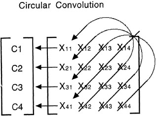
FIG. 5.8. Circular convolution operation used to bind pairs of vectors.
Tensor products extend a model in space because representing a binding between two elements, each of which is represented by an N-dimensional vector, requires N2 units. Circular convolution representations extend the model in space more subtly. Each binding between vectors occupies only N units, but the use of many N-dimensional vectors to bind elements together requires a high-dimensional space so that vectors do not interfere with each other. At most, N orthogonal vectors (which do not interfere with each other) can be placed in an N-dimensional space. If the vector elements are randomly generated, the capacity of such networks is generally much lower (often around 10% of the dimensionality).
A second way of extending connectionist models to incorporate structure is to extend them in time. In these models, the structure unfolds over time in processing. One type of extension uses recurrent networks (Elman, 1990; J. B. Pollack, 1990). Figure 5.9 shows two types of recurrent network architectures. In each case, a new input is associated with some output through a layer of hidden units using the back-propagation learning routine (Rumelhart, Hinton, & Williams, 1986). Back propagation extends the simple learning procedure described in chapter 2 to permit more complex sets of associations. The key aspect of recurrent networks is that a set of context units is added to the network. The first time an association is learned, an arbitrary pattern is given to the context units. For each subsequent association, the previous pattern on either the output units or the hidden units is used as a context. This use of context allows the network to encode sequences and retrieve them later. The sequences are not available all at once but must be decoded over time by reinstating an old context and finding the output associated with it. The retrieved context units can be fed back as input to retrieve the whole sequence. Thus, the extension of these models in time makes the structure in the representation available to the system only over the course of processing and not at any individual moment.
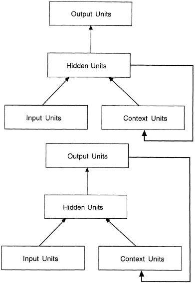
FIG. 5.9. Two architectures for recurrent connectionist models. In the top architecture, the hidden units are used as context; in the bottom architecture, the output units are used as context.
For example, I can teach a recurrent network to produce the letters of the alphabet in order. To do this task, I give an input pattern for the beginning of the sequence, with no values on the context units. I associate this input with a pattern for the letter a. In this way, the model learns that the beginning of the sequence was the letter a. Then, I associate my context units (say the pattern of activation in the hidden units from the previous trial), along with the pattern for the letter a, with the letter b. I continue training in this way, until I reach the end of the alphabet. After these associations are learned, I can retrieve the letters of the alphabet in order by giving the model the input pattern for the beginning of the sequence on the input units, to yield the association a. Then I can generate the rest of the sequence by feeding the context units and the output back to the input units and finding the next learned association.
A final way to represent structure in a connectionist model is the use of temporal binding of units (Hummel & Biederman, 1992; Hummel & Holyoak, 1997; Shastri & Ajjanagadde, 1993). This model differs from distributed connectionist models because it uses a localist representation scheme. Like the parallel constraint satisfaction models described in chapter 4, localist representations assume that each unit has some meaning. Figure 5.10 shows a sample network. To represent a proposition like loves (John, Mary), the system must have units for the relation loves and the objects John and Mary. The system must also have units for the relational roles of loves (e.g., the love-agent and love-patient units in Figure 5.10). The binding between relations and arguments occurs over time. In particular, it is assumed that units active at the same time are bound together. Thus, at one time, the units for loves, love-agent, and John are active together (Figure 5.10B). At another time, the units for loves, love-patient, and Mary are active together (Figure 5.10C). Other relations are represented by other patterns of unit activation. As for recurrent networks, temporal synchrony as a method of binding makes the structure in the representation over time.
As demonstrated in this section, extensions to connectionist models allow them to encode structured representations. Extensive research has been devoted to examining the uses of these structured representations. They have been used successfully as models of data from memory experiments (Metcalfe, 1991, 1993; Metcalfe-Eich, 1982). Workers have achieved some success in developing models of reasoning (Shastri & Ajjanagadde, 1993) and analogical mapping (Halford, Wilson, Guo, Wiles, & Stewart, 1994; Hummel & Holyoak, 1997), although these models often do not perform to the level of existing symbolic models (Gentner & Markman, 1993, 1995). The thrust of this section, however, is that just because some cognitive processes involve structured representations, this fact should not be taken as evidence of the inappropriateness of connectionist models as models of cognition. Instead, it is possible to implement structured representations using connectionist mechanisms.
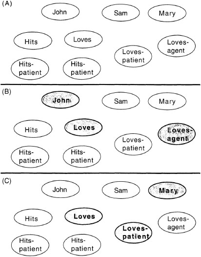
FIG. 5.10. Example of dynamic binding by temporal synchrony. A: Localist connectionist units. B: Units active at the same time representing that John is the agent of a Loves relation. C: Units active at the same time representing that Mary is the patient of a Loves relation.
SUMMARY
Structured representations contain explicit connections between elements. These bindings provide information about the scope of representational elements. Representational structure allows elements to be combined by entering them as arguments of other elements. Structured representations also permit systematicity in which higher order relational structures are developed to represent important information (like causal relations).
The use of structured representations requires more complex processes than did the simpler representations discussed in chapters 2 to 4. Simply comparing a pair of such representations requires a structural alignment process that attends to the bindings between predicates and their arguments. The advantage of such complexity is that this representation process pair can account for the fact that people distinguish between alignable differences (which are related to commonalities) and nonalignable differences (which are not). This process, however, is computationally expensive; when many comparisons must be carried out, a simpler representation and process may be required.
Finally, structured representations can be implemented in different ways. Most examples in this chapter focused on predicate calculus representations, in which symbols were concatenated to form representational structures. Another prominent representational system is frames, which are based on the attribute-value structure of objects. Finally, it is also possible to extend connectionist models in either time or space to account for structure in representations. In the next two chapters, I examine the applications of structured representations to perceptual representation (chap. 6) and conceptual representation (chap. 7).
1Exactly which direction the links should point is a matter of some debate. In this book, I assume that the links point from the predicate to its arguments.
2The attributes of objects are omitted from these representations for clarity. It is assumed that placing a pair of objects in correspondence also places the attributes in correspondence. Similar objects are seen as similar because they have matching attributes.
3This representation is meant to illustrate the use of quantifiers. A predicate like wants-to-hurt (?x, ?y) is too fine grained to be useful. In a working system, it is better to decompose this complex predicate into a set of basic predicates, each of which is useable in a range of representations. This decomposition easily shows the similarity between different representations (e.g., one can recognize that wants-to-hurt [?x, ?y] and wants-to-dance-with [?x, ?y] both involve desire). It becomes complicated to say that a state of affairs is desired without embedding one predicate inside another, but such embedding is not allowed in a first-order logic. One way to do this embedding is to define the event hurts (?x, ?y), to posit the existence of some element z that is the event hurts (?x, ?y), and then to state that x desires z. This would change the sentence in Example 5.15 to ∃ (?x), ∃ (?y), ∃ (?z): person (?x) and person (?y) and event [?z, hurts (?x, ?y) and desires (?x, ?z) where event [?x, ?y) is a predicate that defines the first argument to be an event.
4The same issue discussed in footnote 4 applies to Example 5.16 as well. To represent Example 5.16 using more general predicates, one creates a new event of going home occurring now and then states that person x does not want this event to take place. For example, not [∃ ?x), ∃ ?y) person ?x) and event ?y, go-home ?x]) and (desire ?x, ?y])].
5Even this representation is flawed, because it does not do a good job of representing the temporal aspects of the situation. For example, person y was not hurt before the event but is hurt afterward. To remedy this situation, I can add some time point (call it t) such that before time t person y is not hurt, and after time t y is hurt. This solution allows reasoning about temporal relations among events (see Charniak & McDermott, 1986).
6Actually two different things have been called systematicity in the cognitive science literature. Gentner’s (1983, 1989) sense of systematicity is that the similarity of two domains is thought to be higher when these domains match along higher order relational structure than if they match along only isolated first-order relations. The second use of systematicity is also related to structured representations (J. A. Fodor & Pylyshyn, 1988). This use of systematicity says that the ability to think some thoughts is lawfully connected to the ability to think other thoughts. For example, if I can think the thought “John kissed Mary,” I can also think the thought “Mary kissed John.” According to Fodor and Pylyshyn, this systematicity arises because mental representations are structured and compositional (i.e., the components can be freely combined). For example, “John kissed Mary” can be represented as kissed (John, Mary). There should be no problem reversing the arguments to this relation to yield kissed (Mary, John) or “Mary kissed John.” Although both terms address aspects of structured representations, they are not quite the same aspect.
7Perner (1991) provided an interesting discussion of the minimum representational abilities that a child must have to be able to properly solve particular false belief tasks.
8Some implementational details must be incorporated into the models to get them to work. For example, the elements of each vector must be created so that the activation of its units is independently distributed with a mean of 0 and a variance of 1/N (where N is the number of dimensions). This distribution is necessary because there is no unique mapping between a circular convolution and a single pair of vectors creating it.