
Chapter 9
Quantifying and Analyzing Project Risk
“Knowledge is power.”
—FRANCIS BACON
Information is central to managing projects successfully. Knowledge of the work and potential risk serves as the first and best defense against problems and project delay. The overall assessment of project risk provides concrete justification for necessary changes in the project objective, so it is one of the most powerful tools you have in transforming an impossible project into one that can be successful. Project-level risk rises steeply for projects with insufficient resources or excessively aggressive schedules, and risk assessments offer compelling evidence of the exposure this represents. Knowledge of project risk also sets expectations for the project appropriately, both for the deliverables and for the work that lies ahead. The focus of this chapter is analyzing overall project risk, building on the foundation of analysis and response planning for known activity risks discussed in Chapters 7 and 8.
Project-Level Risk
Considered one by one, the known risks on a project may seem relatively easy to deal with, overwhelming, or somewhere in between. Assessing risk at the activity level is necessary, but it is not sufficient; you also need to develop a sense of overall project risk. Overall project risk arises, in part, from all the aggregated activity-level risk data, but it also has a component that is more pervasive, coming from the project as a whole. High-level project risk assessment was discussed in Chapter 3, using methods that required only information available during initial project definition. Those high-level techniques—the risk framework, the risk complexity index, and the risk assessment grid—may also be reviewed and revised based on your project plans.
As the preliminary project planning process approaches completion, you have much more information available, so you can assess project risk more precisely and thoroughly. There are a number of useful tools for assessing project risk, including statistics, metrics, and modeling and simulation tools. Risk assessment using planning data may be used to support decisions, to recommend project changes, and to better control and execute the project.
Some sources of overall project risk include:
• Unrealistic deadlines: High-tech projects often have inappropriately aggressive schedules.
• No or few metrics: Measures used for estimates and risk assessment are inaccurate guesswork.
• “Accidental” project leaders: Projects are led by team members skilled in technical work but with no project management training.
• Inadequate requirements and scope creep: Poor initial definition and insufficient specification change control are far too common.
• Project size: Project risk increases with scale; the larger the project, the more likely it is to fail.
Some of these project-level risks are well represented in the PERIL database, and methods for determining overall project risk can be effective in both lowering their impact and determining a project’s potential for trouble. In addition, overall risk assessment scores can:
• Build support for less risky projects and cause cancellation for some higher-risk projects
• Compare projects and help set relative priorities
• Provide data for renegotiating overconstrained project objectives
• Assist in determining required management reserve
• Facilitate effective communication and build awareness of project risk
The techniques, tools, ideas, and metrics described in this chapter address these issues.
Aggregating Risk Responses
One way to assess project risk is to add up all the expected consequences of all of the project risks. This is not just a simple sum; the total is based on the estimated cost (or time) involved multiplied by the risk probability—the “loss times likelihood” aggregated for the whole project.
One way to calculate project-level risk is by accumulating the consequences of the contingency plans. For this, sum the “expected” costs for all the plans—their estimated costs weighted by the risk probabilities. Similarly, you can calculate the total expected project duration increase required by the contingency plans using the same probability estimates. For example, if a contingency plan associated with a risk having a 10 percent probability will cost $10,000 and slip the project by ten days, the contribution to the project totals will be $1,000 and one day (assuming the activity is critical), respectively.
Another way to generate similar data is by using the differences between Program Evaluation and Review Technique (PERT)-based expected estimates and the “most likely” activity estimates. Summing these estimates of both cost and time impact for the project generates an assessment roughly equivalent to the contingency plan data.
Although these sums of expected consequences provide a baseline for overall project risk, they will tend to underestimate total risk, for a number of reasons. First, this analysis assumes that all project risks are independent, with no expected correlation. The assumption of negligible correlation is generally incorrect for real projects; most project risks become much more likely after other risks have occurred. Project activities are linked through common methodologies, staffing, and other factors. Also, projects have a limited staff, so whenever there is a problem, nearly all of the project leader’s attention (and much of the project team’s) will be on recovery. Distracted by problem solving, the project leader will focus much less on all the other project activities, making additional trouble elsewhere that much more likely.
Another big reason that overall project risk is underestimated using this method is that the weighted sums fail to account for project-level risk factors. Overall project-level risk factors include:
• Inexperience of project manager
• Weak sponsorship
• Reorganization, business changes
• Regulatory issues
• Lack of common practices (life cycle, planning, and so forth)
• Market window or other timing assumptions
• Insufficient risk management
• Ineffective project decomposition resulting in inefficient work flow
• Unfamiliar levels of project effort
• Low project priority
• Poor motivation and team morale
• Weak change management control
• Lack of customer interaction
• Communications issues
• Poorly defined infrastructure
• Inaccurate (or no) metrics
The first two factors on the list are particularly significant. If the project leader has little experience running similar projects successfully, or the project has low priority, or both, you can increment the overall project risk assessment from summing expected impacts by at least 10 percent, for each. Similarly, make adjustments for any of the other factors that may be significant for the project. Even after these adjustments, the risk assessment will still be somewhat conservative, because “unknown” project risk impacts are not included.
Compare the total expected project duration and cost impacts related to project risks with your preliminary baseline plan. Whenever the expected risk impact for either time or cost exceeds 20 percent of your plan, the project is very risky. This project risk data on cost and schedule impact is useful for negotiating project adjustments, justifying management reserve, or both.
Questionnaires and Surveys
Questionnaires and surveys are a well-established technique for assessing project risk. These can range from simple, multiple-response survey forms, to assessments using computer spreadsheets, Web surveys, or other computer tools. However you choose to implement a risk assessment survey, it will be most effective if you customize it for your project.
Many organizations have and use risk surveys. If there is a survey or questionnaire commonly used for projects similar to yours, there may be very little customizing required. Even if you have a format available, it is always a good idea to review the questions and fine-tune the survey before using it. If you do not have a standard survey format, the following example is a generic three-option risk survey that can be adapted for use on a wide range of technical projects.
This survey approach to risk assessment also works best when the number of total questions is kept to a minimum, so review the format you intend to use and select only the questions that are most relevant to your project risks. An effective survey may not need to probe more than about a dozen key areas—never more than about twenty. If you plan to use the following survey, read each of the questions and make changes as needed to reflect your project environment. Strike out any questions that are irrelevant, and add new questions if necessary to reflect risky aspects of your project. Effective surveys are short, so delete any questions that seem less applicable. If you develop your own survey, limit the number of responses for each question to no more than four clearly worded responses.
Once you have finalized the risk assessment questionnaire, the next step is to get input from each member of the core project team. Ask each person who participated in project planning to respond to each question, and then collect his or her data.
Risk survey data is useful in two ways. First, you can analyze all the data to produce an overall assessment of risk. This can be used to compare projects, to set expectations, and to establish risk reserves. Second, you can scan the responses question by question to find particular project-level sources of risk—questions where the responses are consistently in the high-risk category. Risk surveys can be very compelling evidence for needed changes in project infrastructure or other project factors that increase risk. For high-risk factors, ask, “Do we need to settle for this? Is there any reason we should not consider changes that will reduce project risk?” Also investigate any questions with widely divergent responses, and conduct additional discussions to establish common understanding within the project team.
Instructions for the Project Risk Questionnaire
Before using the following qualitative survey, read each one of the questions and make changes as needed to reflect your project environment. Eliminate irrelevant questions and add new ones if necessary to reflect risky aspects of your project. Effective surveys are short, so limit the survey to ten to twenty total questions. Section 2, “Technical Risks,” normally requires the most intensive editing. The three sections focus on:
1. Project external factors (such as users, budgets, and schedule constraints)
2. Development issues (such as tools, software, and hardware)
3. Project internal factors (such as infrastructure, team cohesion, and communications)
Distribute copies to key project contributors and stakeholders and ask each person to select one of the three choices offered for each question. To interpret the information, assign values of 1 to selections in the first column, 3 to selections in the middle column, and 9 to selections in the third column. Within each section, sum up the responses, then divide each sum by the number of responses tallied. Within each section, use the following evaluation criteria:
• Low risk: 1.00 to 2.50
• Medium risk: 2.51 to 6.00
• High risk: 6.01 to 9.00
Average all questions to determine overall project risk, using the same criteria. Although the results of this kind of survey are qualitative, they can help you to identify sources of high risk in your project. For any section with medium or high risk, consider changes to the project that might lower the risk. Within each section, look for responses in the third column. Brainstorm ideas, tactics, or project changes that could shift the response, reducing overall project risk.
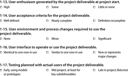
Risk Questionnaire
For each question below, choose the response that best describes your project. If the best response seems to lie between two choices, check the one of the pair further to the right.
Section 1. Project Parameter and Target User Risks
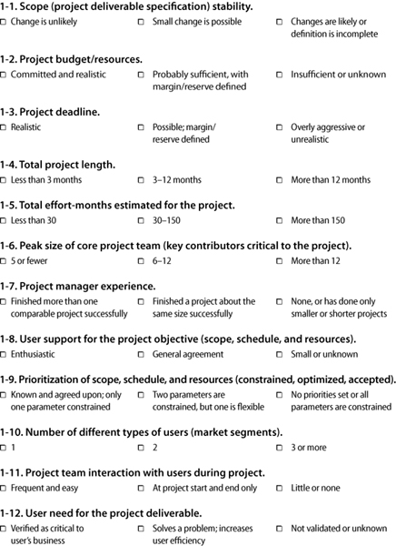
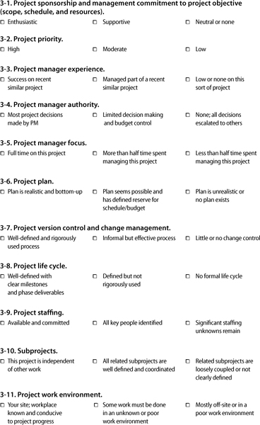
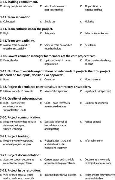
Section 2. Technical Risks

Section 3. Structure Risks
Project Simulation and Modeling
Most project modeling methodologies may be traced back to the PERT, discussed in Chapter 4 with regard to estimating and in Chapter 7 for analysis of activity risk. Although the applications discussed earlier are useful, they were related to project activities. The original purpose of PERT was to quantify project risk, which is the topic of this chapter. There are several approaches to using PERT and other simulation and decision analysis techniques for project risk analysis.
PERT for Project Risk Analysis
PERT was not developed by project managers. It was developed in the late 1950s at the direction of U.S. military to deal with the increasingly common cost and schedule overruns on very large U.S. government projects. The larger the programs became, the bigger their overruns. Generals and admirals are not patient people, and they hate to be kept waiting. Even worse, the U.S. Congress got involved whenever costs exceeded the original estimates, and the generals and admirals liked that even less.
The principal objective of PERT was to use detailed risk data at the activity level to predict project outcomes. For schedule analysis, project teams were requested to provide three estimates: a “most likely” estimate that they believe would be the most common duration for work similar to the activity in question, and two additional estimates that define a range around the “most likely” estimate with a goal of including all realistic possibilities for work duration.
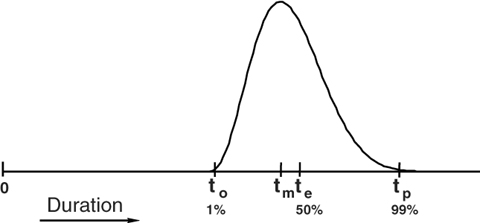
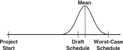
Shown in Figure 9-1, the three PERT time estimates are: At the low end, an “optimistic” estimate, to; in the middle somewhere, a “most likely” estimate, tm; and at the high end, a “pessimistic” estimate, tp.
Originally, PERT analysis assumed a continuous Beta distribution of outcomes defined by these three parameters, similar to the graph in Figure 9-1. This distribution was chosen because it is relatively easy to work with, and it can skew to the left (as in Figure 9-1) or to the right based on the three estimating parameters. (When the estimates are symmetric, the Beta distribution is equivalent to the normal distribution: the Gaussian, bell-shaped curve.)
Some issues with PERT were discussed in the earlier chapters, but there is an additional issue with PERT for project schedule analysis. PERT uses simple approximations for estimating expected durations and tends to underestimate project risk, especially for projects having more than one critical path. Based on the weighted averages, PERT expected durations can be used to perform standard critical path methodology (CPM) analysis. The resulting project will have a longer expected path, but analysis using computer simulation will provide a more useful assessment of overall project schedule impact. Computer simulation uses pseudo-random number generation to calculate a duration within each activity range estimate and repeats the process over and over, each time using new activity duration estimates. CPM is used to calculate the project’s critical path for each of these new schedules, and over many repetitions this simulation builds a histogram of the results.
Today’s computer simulation and modeling tools for project management offer many alternatives to the Beta distribution. You may use triangular, normal, Poisson, and many other distributions, or even histograms defining discrete estimates with associated probabilities. (For example, you may expect a 50 percent probability that the activity will complete in 15 days, a 40 percent chance that it will complete in 20 days, and a 10 percent chance that it will complete in 30 days. These scenarios are generally based on probabilities associated with known risks for which “worst-case” incremental estimates are made—the five-day slip associated with a contributor who may need to take a week of leave to deal with a family situation, the fifteen-day slip associated with a problem that requires completely redoing of all the work.)
As discussed in Chapter 7, the precise choice of the distribution shape is not terribly important, even for activity-level risk analysis. At the project level, it becomes even less relevant. The reason for this is that the probability density function for the summation of randomly generated samples of most types of statistical distributions (including all the realistic ones) always resembles a normal, bell-shaped, Gaussian distribution. This is due to the central limit theorem, well established by statisticians, and it is why the analysis for a project with a single, dominant critical path always resembles a symmetric, bell-shaped curve. The normal distribution has only two defining parameters, the mean and the variance (the square of the standard deviation). For the Beta distribution the mean and standard deviation are estimated with the formulas referenced earlier:
te = (to + 4tm + tp)/6, where
te is the “expected” duration—the mean
to is the “optimistic” duration
tm is the “most likely” duration
tp is the “pessimistic” duration
and
σ = (tp – to)/6, where
σ is the standard deviation
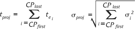
For a project with a single, dominant critical path, the expected duration for the project is the sum of all the expected (mean) durations along the critical path. The standard deviation for such a project, one measure of overall project risk, can be calculated from the estimated standard deviations for the same activities. PERT used the following formulas:
where:
tproj = Expected project duration
CPi = Critical path activity i
tei = “Expected” CP estimate for activity i
σproj = Project standard deviation
σ2i = Variance for CP activity i
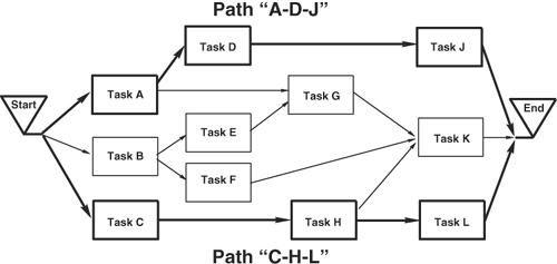
These formulas work well whenever there is a single critical path, but it gets more complicated when there are additional paths that are roughly equivalent in length to the longest one. When this occurs, the PERT formulas will underestimate the expected project duration (it is actually slightly higher) and they will overestimate the standard deviation. For such projects, computer simulation will provide better results than the PERT approximations. The main reason for this inaccuracy was introduced in Chapter 4, in the discussion of multiple critical paths. There, the distinction between “Early/On time” and “Late” was a sharp one, with no allowance for degree. Simulation analysis using distributions for each activity creates a spectrum of possible outcomes for the project, but the logic is the same—more failure modes lead to lowered success rates. Because any of the parallel critical paths may end up being the longest for each simulated case, each contributes to potential project slippage. The simple project considered in Chapter 4 had the network diagram in Figure 9-2, with one critical path across the top (“A-D-J”) and a second critical path along the bottom (“C-H-L”).
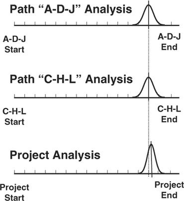
CPM and PERT analysis, as should be expected, show that there is about one chance in four that the project will complete on time or earlier than the expected durations associated with each of the critical paths. The distribution of possible outcomes for the project has about one-quarter of the left tail below the expected dates, and the peak and right tail are above it, similar to Figure 9-3. The resulting distribution is still basically bell-shaped, but compared with the distributions expected for each critical path, it has a larger mean and is narrower (a smaller standard deviation).
To consider this quantitatively, imagine a project plan using “50 percent” expected estimates that has a single dominant critical path of 100 days (5 months) and a standard deviation of 5 days. (If the distribution of expected outcomes is assumed symmetric, the PERT optimistic and pessimistic durations—plus or minus three standard deviations—would be roughly 85 days and 115 days, respectively.) PERT analysis for the project says you should expect the project to complete in five months (or sooner) five times out of ten and in five months plus one week over eight times out of ten (about 5/6 of the time)—pretty good odds.
Figure 9-2. Project with two critical paths.
If a second critical path of 100 days is added to the project with similar estimated risk (a standard deviation of 5 days), the project expectation shifts to 1 chance in 4 of finishing in 5 months or sooner. (Actually, the results of the simulation based on 1,000 runs shows 25.5 percent. The results of simulation almost never exactly match the theoretical answer.) In the simulation, the average expected project duration is a little less than 103 days, and the similar “5/6” point is roughly 107 days. This is a small shift (about one-half week) for the expected project, but it is a very large shift in the probability of meeting the date that is printed on the project Gantt chart—from one chance in two to one chance in four (as expected).
Similar simulations for three and four parallel critical paths of equivalent expected duration and risk produce the results you would expect. For three paths of 100 days, the project expectation falls to one chance in eight of completing on or before 100 days (a simulation of this showed 13 percent) and an expected duration of roughly 104 days. The project with four failure modes has one chance in sixteen (6.3 percent in the model), and the mean for the project is a little bit more than 105 days. The resulting histogram for this case is in Figure 9-4, based on 1,000 samples from each of four independent, normally distributed parallel paths with mean of 100 days and a standard deviation of 5 days. (The jagged distribution is typical of simulation output.)
For these multiple–critical path cases, the mean for the distribution increases, and the range compresses somewhat, reducing the expected standard deviation. This is because the upper data boundary for the analysis is unchanged, while each additional critical path will tend to further limit the effective lower boundary. For the case in Figure 9-4, the project duration is always the longest of the four, and it becomes less and less likely that this maximum will be near the optimistic possibilities with each added path. Starting with a standard deviation for each path of five days, the resulting distribution for a project with two similar critical paths has a standard deviation of about 4.3 days. For three paths it is just under four days, and with four it falls to roughly 3.5 days, the result from the example in Figure 9-4. The resulting distributions also skew slightly to the left, for the same reasons; the data populating the histograms is being compressed, but only from the lower side.
Computer simulation analysis of this sort is most commonly performed for duration estimates, but effort and cost estimates may also be used. As with schedule analysis, three-point cost estimates may be used to generate expected activity costs, and sum them for the entire project. Because all costs are cumulative, the PERT cost analysis formulas analogous to those for time analysis deliver results equivalent to simulation.

Using Computer Simulation
Simulation analysis uses computers, and for this reason it was impractical before the 1960s (which is why PERT depended on simplified approximations). Once computer-based analysis was practical, Monte Carlo simulation techniques began to be widely used to analyze many kinds of complex systems, including projects. Initially, this sort of analysis was very expensive (and slow), so it was undertaken only for the largest, most costly projects. This is no longer an issue with today’s inexpensive desktop systems.
The issue of data quality for schedule risk analysis was also significant in early implementations, and this drawback persists. Generating range estimates remains difficult, especially when defined in terms of “percent tails” as is generally done when describing three-point estimates in the project management literature. Considering that the initial single-point “most likely” estimates are generally not very precise or reliable, the two additional upper and lower boundary estimates are likely to be even worse. Because at least some of the input data is inexact, the “garbage in/garbage out” problem is a standard concern with Monte Carlo schedule analysis.
This, added to the temptation for misuse of the “optimistic” estimates by overeager managers and project sponsors, has made widespread use of computer simulation for technical projects difficult. This is unfortunate, because even if range estimate analysis is applied to suspected critical activities using only manual approximations, it can still provide valuable insight into the level of project risk. Some effective methods require only modest additional effort, and there are a number of techniques, from manual approximations to full computer simulation. A summary of choices appears in the next few sections.
Manual approximations One way to apply these concepts was discussed earlier in this book. If you have a project scheduling tool, and project schedule information has been entered into the database, most of the necessary work is already done. The duration estimates in the database are a reasonable first approximation for the optimistic estimates, or the most likely estimates (or both). To get a sense of project risk, make a copy of the database and enter new estimates for every activity where you have a worst-case or a pessimistic estimate. The Gantt chart based on these longer estimates will display end points for the project that are further out than the original schedule. By associating a normal distribution with these points, a rough approximation of the output for a PERT analysis may be inferred.
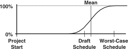
The method used for scaling and positioning the bell-shaped curve can vary, but at least half of the distribution ought to fall between the lower “likely” boundary and the upper “pessimistic” limits defined by the end points of the two Gantt charts. Because it is very unlikely that all the things that could go wrong in the project will actually happen, the upper boundary should line up with a point several standard deviations from the mean, far out on the distribution tail. (Keep in mind, however, that this accounts for none of your unknown project risk.) The initial values in the scheduling database are probably somewhere below the mean of the distribution, though the exact placement should be a function of perceived accuracy for your estimates and how conservative or aggressive the estimates are. A histogram similar to Figure 9-5, using the initial plan as about the 20 percent point (roughly one standard deviation below the mean) and the worst-case plan to define the 99 percent point (roughly three standard deviations above the mean), is not a bad first approximation.
If the result represented by Figure 9-5 looks unrealistic, it may improve things if you calculate expected estimates, at least for the riskiest activities on or near a critical path. If you choose to do the arithmetic, a third copy of the database can be populated with expected estimates, defining the mean (the “50 percent” point) for the normal distribution. The cumulative graph of project completion probabilities equivalent to Figure 9-5 looks like Figure 9-6.
Although this sort of analysis is still subjective, the additional effort it requires is small once you generate a preliminary schedule for the project, and it provides valuable insight regarding project risk.
One of the most important things about techniques that make schedule risk visible is that they provide a very concrete, specific result. The results of this analysis will either look reasonable to you or they will seem “wrong.” If the results seem realistic, they are probably useful. If they look unrealistic, it usually indicates that additional work and planning is warranted. Improbable-looking results are a good indication that your activity list is incomplete, your estimates are inaccurate, you missed some dependencies, you underestimated some risks, or your preliminary plan has some other defect.
Figure 9-5. “PERT” approximation.
Even this “quick and dirty” type of schedule risk approximation provides insight into the thoroughness of your project plan.
Computer spreadsheets The next step up in sophistication involves a computer spreadsheet. This is particularly useful for resource analysis, where everything is cumulative. Spreadsheets are a very easy way to quickly assess three cost (or effort) estimates to derive an overall project-level budget analysis. A list of all the activities in one column with the “most likely” and range estimates in adjacent columns can be readily used to calculate expected estimates and variances for each activity and for the project as a whole. Using the PERT formulas for cost, it is simple to accumulate and evaluate data from all the project activities (not just from the critical path). The sum of all the expected costs and the calculated variance can be used to approximate project budget risk. Assuming a normal distribution centered on the sum of the expected cost estimates with a spread defined by the calculated standard deviation shows the range that may be expected for project cost.
For the reasons outlined earlier, similar duration estimate analysis will underestimate the expected project duration and overestimate the standard deviation, but it could be useful for a simple or small project.
Computer scheduling tools True Monte Carlo simulation analysis capability is not common in most computer-based scheduling tools, and what is available to support three-point activity duration estimates tends to be implemented in quirky and mysterious ways. It is impractical to list all the available scheduling tools here, so the following discussion characterizes them generically.
There are dozens of such tools available for project scheduling, ranging from minimalist products that implement rudimentary activity analysis to high-end, Web-enabled enterprise applications. Often, families of software offering a range of capabilities are sold by the same company. Almost any of these tools may be used for determining the project critical path, but schedule risk analysis using most of these tools, even some fairly expensive ones, often requires the manual processes discussed already or purchase of additional, specialized software (more on this specialized software follows). In general, scheduling tools are set up for schedule analysis using single-point estimates to determine critical path, and three-point estimate analysis requires several copies of the project data (or a scratch pad version for “what if?” analysis) to analyze potential schedule variance. Some products do provide for entry of three-point estimates and some rudimentary analysis, but this is typically based on calculations (as with PERT), not simulation.
Some high-end project management tools, which are both more capable and more costly than the more ubiquitous midrange tools, do provide integrated Monte Carlo simulation analysis, either built-in or as optional capabilities. Even with the high-end tools, though, schedule simulation analysis requires an experienced project planner with a solid understanding of the process.
Computer simulation tools Tools that provide true Monte Carlo simulation functionality are of two types, designed either to be integrated with a computer scheduling tool or for stand-alone analysis. Again, there are many options available in both of these categories.
There are quite a few applications designed to provide simulation-based risk analysis that either integrate into high-end tools or “bolt on” to midrange scheduling packages. If such an add-on capability is available for the software you are using, simulation analysis can be done without having to reenter or convert any of your project data. With the stand-alone software, project information must be input a second time or exported. Unless you also need to do some nonproject simulation analysis, Monte Carlo simulation tools designed to interface directly with scheduling applications are generally a less expensive option.
In addition to products specifically designed for Monte Carlo schedule analysis, there are also general-purpose simulation applications that could be used, including decision support software and general-purpose statistical analysis software. For the truly masochistic, it is even possible to do Monte Carlo simulations using only a spreadsheet—Microsoft Excel includes functions for generating random samples from various distribution types as well as statistical analysis functions for interpreting the data.
Whatever option you choose, there are trade-offs. Some techniques are quick and relatively easy to implement, providing subjective but still useful insight into project risk. Other, full-function Monte Carlo methods offer very real risk management benefits, but they also carry costs, including investment in software, generation of more data, and increased effort. Before deciding to embark on an elaborate project Monte Carlo simulation analysis, especially the first time, carefully consider the costs and added complexity.
A primary benefit of any of this risk analysis is the graphic and visible contrast between the deterministic-looking schedule generated by point-estimate critical path methods, and the range of possible end points (and associated probabilities) that emerge from these methods. The illusion of certainty fostered by single-estimate Gantt charts is inconsistent with the actual risk present in technical projects. The visible variation possible in a project is a good antidote for excessive project optimism.
Also, keep in mind that precise-looking output may create an illusion of precision. The accuracy of the output generated by these methods can never be any better than that of the least precise inputs. Rounding the results off to whole days is about the best you can expect, yet results with many decimal places are reported, especially by Monte Carlo simulation software. This is particularly ironic considering the quality of typical project input data. Generating useful estimates and the effort of collecting, entering, and interpreting this risk information represents quite a bit of work.
In project environments that currently lack systematic project-level risk analysis, it may be prudent to begin with a modest manual approximation effort on a few projects, and expand as necessary for future projects.
Analysis of Scale
Quantitative project analysis using all the preceding techniques, with either computer tools or manual methods, is based on details of the project work—activities, worst cases, resource issues, and other planning data. It is also possible to assess risk based on the overall size of the project, because the overall level of effort is another important risk factor. Projects only 20 percent larger than previous work represent significant risk.
Analysis of project scale is based on the overall effort in the project plan. Projects fall into three categories—low risk, normal risk, and high risk—based on the anticipated effort compared with earlier, successful projects. Scale assessment begins by accumulating the data from the bottom-up project plan to determine total project effort, measured in a suitable unit such as “effort-months.” The calculated project scale can then be compared with the effort actually used on several recent, similar projects. In selecting comparison projects, look for work that had similar deliverables, timing, and staffing so the comparison will be as valid as possible. If the data for the other projects is not in the form you need, do a rough estimate using staffing levels and project duration. If there were periods in the comparison projects where significant overtime was used, especially at the end, account for that effort as well. The numbers generated do not need to be precise, but they do need to fairly represent the amount of overall effort actually required to complete the comparison projects.
Using the total of planned effort-months for your project and an average from the comparison projects, determine the risk:
• Low risk: Less than 60 percent of the average
• Normal risk: Between 60 percent and 120 percent of the average
• High risk: Greater than 120 percent of the average
These ranges center on 90 percent rather than 100 percent because the comparison is between actual past project data, which includes all changes and risks that occurred, and the current project plans, which do not. Risk arises from other factors in addition to size, so consider raising the risk assessment one category if:
• The schedule is significantly compressed
• The project requires new technology
• 40 percent of the project resources are either external or unknown
Project Appraisal
Analysis of project scale can be taken a further step, both to validate the project plan and to get a more precise estimate of risk. The technique requires an “appraisal,” similar to the process used whenever you need to know the value of something, such as a piece of property or jewelry, but you do not want to sell it to find out. Value appraisals are based on the recent sale of several similar items, with appropriate additions and deductions to account for small differences. If you want to know the value of your home, an appraiser examines it and finds descriptions of several comparable homes recently sold nearby. If the comparison home has an extra bathroom, a small deduction is made to its purchase price; if your house has a larger, more modern kitchen, the appraiser makes a small positive adjustment. The process continues, using at least two other homes, until all factors normally included are assessed. The average adjusted price that results is taken to be the value of your home—the current price for which you could probably sell it.
The same process can be applied to projects, because you face a similar situation. You would like to know how much effort a project will require, but you cannot wait until all the work is done to find out. The comparisons in this case are two or three recently completed similar projects, for which you can ascertain the number of effort-months that were required for each. (This starts with the same data the analysis of scale technique uses.)
From your bottom-up plan, calculate the number of effort-months your project is expected to take. The current project can be compared to the comparison projects, using a list of factors germane to your work. Factors relevant to the scope, schedule, and resources for the projects can be compared, as in Figure 9-7 (which was quickly assembled using a computer spreadsheet).
One goal of this technique is to find comparison projects that are as similar as possible, so the adjustments will be small and the appraisal can be as accurate as possible. If a factor seems “similar,” no adjustment is made. When there are differences, adjust conservatively, such as:
Figure 9-7. Project appraisal.

• Small differences: Plus or minus 2 to 5 percent
• Larger differences: Plus or minus 7 to 10 percent
The adjustments are positive if the current project has the higher risk and negative if the comparison project seems more challenging.
The first thing you can use a project appraisal for is to test whether your preliminary plan is realistic. Whenever the adjusted comparison projects average to a higher number of effort-months than your current planning shows, your plan is almost certainly missing something. Whenever the appraisal indicates a difference greater than about 10 percent compared with the bottom-up planning, work to understand why. What have you overlooked? Where are your estimates too optimistic? What activities have you not captured? Also, compare the project appraisal effort-month estimate with the resource goal in the original project objective. A project appraisal also provides early warning of potential budget problems.
One reason project appraisals will generally be larger than the corresponding plan is because of risk. The finished projects include the consequences of all risks, including those that were invisible early in the work. The current project planning includes data on only the known risks for which you have incorporated risk prevention strategies. At least part of the difference between your plan and an appraisal is due to the comparison projects’ “unknown” risks, contingency plans, and other risk recovery efforts.
In addition to plan validation, project appraisals are useful in project-level risk management. Whenever there is a major difference between the parameters of the planned project and the goals stated in the project objective, the appraisal shows why convincingly and in a very concise format.
A project appraisal is also a very effective way to initiate discussion with your project sponsor of options, trade-offs, and changes required for overconstrained projects, which is addressed in Chapter 10.
Project Metrics
Project measurement is essential to risk management. It also provides the historical basis for other project planning and management processes such as estimation, scheduling, controlling, and resource planning. Metrics drive behavior, so selecting appropriate factors to measure can have a significant effect on motivation and project progress. HP founder Bill Hewlett was fond of saying, “What gets measured gets done.” Metrics provide the information needed to improve processes and to detect when it is time to modify or replace an existing process. Established metrics also are the foundation of project tracking, establishing the baseline for measuring progress. Defining, implementing, and interpreting a system of ongoing measures is not difficult, so it is unfortunate that on many projects it either is not done at all or is done poorly.
Establishing Metrics
Before deciding what to measure, carefully define the behavior you want and determine what measurements will be most likely to encourage that behavior. Next, establish a baseline by collecting enough data to determine current performance for what you plan to measure. Going forward, you can use metrics to detect changes, trigger process improvements, evaluate process modifications, and make performance and progress visible.
The process begins with defining the results or behavior you desire. For metrics in support of better project risk management, a typical goal might be “Reduce unanticipated project effort” or “Improve the accuracy of project estimates.” Consider what you might be able to measure that relates to the desired outcome. For unanticipated project effort, you might measure “Total effort actually consumed by the project versus effort planned.” For estimation accuracy, a possible metric might be “Cumulative difference between project estimates and project results, as measured at the project conclusion.”
Metrics are of three basic types: predictive, diagnostic, and retrospective. An effective system of metrics will generally include measures of more than one type, providing for good balance.
Predictive metrics use current information to provide insight into future conditions. Because predictive metrics are based on speculative rather than empirical data, they are typically the least reliable of the three types. Predictive metrics include the initial assessment of project “return on investment,” the output from the quantitative risk management tools, and most other measurements based on planning data.
Diagnostic metrics are designed to provide current information about a system. Based on the latest data, they assess the state of a running process and may detect anomalies or forecast future problems. The unanticipated effort metric suggested before is based on earned value, a project metric discussed below.
Retrospective metrics report after the fact on how the process worked. Backward-looking metrics report on the overall health of the process and are useful in tracking trends. Retrospective metrics can be used to calibrate and improve the accuracy of corresponding predictive metrics for subsequent projects.
Measuring Projects
The following section includes a number of useful project metrics. No project will need to collect all of them, but one or more measurements of each type of metric, collected and evaluated for all projects in an organization, can significantly improve the planning and risk management on future projects. These metrics relate directly to projects and project management. A discussion of additional metrics, related to financial measures, follows this section.
When implementing any set of metrics, you need to spend some time collecting data to validate a baseline for the measurements before you make any decisions or changes. Until you have a validated baseline, measurements will be hard to interpret, and you will not be able to determine the effects of process modifications that you make. There is more discussion on selecting and using metrics in Chapter 10.
Predictive project metrics Most predictive project metrics relate to factors that can be calculated using data from your project plan. These metrics are fairly easy to define and calculate, and they can be validated against corresponding actual data at the project close. Over time, the goal for each of these should be to drive the predictive measures and the retrospective results into closer and closer agreement. Measurement baselines are set using project goals and planning data.
Predictive project metrics serve as a distant early warning system for project risk. These metrics use forecast information, normally assessed in the early stages of work, to make unrealistic assumptions, significant potential problems, and other project risk sources visible. Because they are primarily based on speculative rather than empirical data, predictive metrics are generally the least precise of the three types. Predictive project measures support risk management in a number of ways:
• Determining project scale
• Identifying the need for risk mitigation and other project plan revisions
• Determining situations that require contingency planning
• Justifying schedule and budget reserves
• Supporting project portfolio decisions and validating relative project priorities
Predictive metrics are useful in helping you anticipate potential project problems. One method of doing this is to identify any of these predictive metrics that is significantly larger than typically measured for past, successful projects—a variance of 15 to 20 percent represents significant project risk. A second use for these metrics is to correlate them with other project properties. After measuring factors such as unanticipated effort, unforeseen risks, and project delays for ten or more projects, some of these factors may reveal sufficient correlation to predict future risks with fair accuracy. Predictive project metrics include:
Scope and Scale Risk
• Project complexity (interfaces, algorithmic assessments, technical or architecture analysis)
• Volume of expected changes
• Size-based deliverable analysis (component counts, number of major deliverables, lines of noncommented code, blocks on system diagrams)
• Number of planned activities
Schedule Risk
• Project duration (elapsed calendar time)
• Total length (sum of all activity durations if executed sequentially)
• Logical length (maximum number of activities on a single network path)
• Logical width (maximum number of parallel paths)
• Activity duration estimates compared with worst-case duration estimates
• Number of critical (or near-critical) paths in project network
• Logical project complexity (the ratio of activity dependencies to activities)
• Maximum number of predecessors for any milestone
• Total number of external predecessor dependencies
• Project independence (ratio of internal dependencies to all dependencies)
• Total float (sum of total project activity float)
• Project density (ratio of total length to total length plus total float)
• Total effort (sum of all activity effort estimates)
• Total cost (budget at completion)
• Staff size (full-time equivalent and/or total individuals)
• Activity cost (or effort) estimates compared with worst-case resource estimates
• Number of unidentified activity owners
• Number of staff not yet assigned or hired
• Number of activity owners with no identified backup
• Expected staff turnover
• Number of geographically separate sites
Financial Risk—Expected Return on Investment (ROI)
• Payback analysis
• Net present value
• Internal rate of return
General Risk
• Number of identified risks in the risk register
• Quantitative (and qualitative) risk assessments
• Adjusted total effort (project appraisal: comparing baseline plan with completed similar projects, adjusting for significant differences)
• Survey-based risk assessment (summarized risk data collected from project staff, using selected assessment questions)
• Aggregated overall schedule risk (or aggregated worst-case duration estimates)
• Aggregated resource risk (or aggregated worst-case cost estimates)
Diagnostic project metrics Diagnostic metrics are based on measurements taken throughout the project, and they are used to detect adverse project variances and project problems either in advance or as soon as is practical. Measurement baselines are generally set using a combination of stated goals and historical data from earlier projects. Diagnostic metrics are comparative measures, either trend-oriented (comparing the current measure with earlier measures) or prediction-oriented (comparing measurements with corresponding predictions, generally based on planning).
Based on project status information, diagnostic project metrics assess the current state of an ongoing project. Risk-related uses include:
• Triggering risk responses and other adaptive actions
• Assessing the impact of project changes
• Providing early warning for potential future problems
• Determining the need to update contingency plans or develop new ones
• Deciding when to modify (or cancel) projects
A number of diagnostic project metrics relate to the concept of earned value management (EVM). These metrics are listed with resource metrics below and described following this list of typical diagnostic project metrics:
Scope Risk
• Results of tests, inspections, reviews, and walkthroughs
• Number and magnitude of approved scope changes
Schedule Risk
• Key milestones missed
• Critical path activity slippage
• Cumulative project slippage
• Number of added activities
• Early activity completions
• Activity closure index: the ratio of activities closed in the project so far to the number expected
Resource Risk
• Excess consumption of effort or funds
• Amount of unplanned overtime
• Earned value (EV): a running accumulation of the costs that were planned for every project activity that is currently complete
• Actual cost (AC): a running accumulation of the actual costs for every project activity that is currently complete
• Planned value (PV): a running accumulation of the planned costs for every project activity that was expected to be complete up to the current time
• Cost performance index (CPI): the ratio of earned value to actual cost
• Schedule performance index (SPI): the ratio of earned value to planned value
• Cost variance (CV): the difference between earned value and actual cost, a measurement of how much the project is over or under budget
• Schedule variance (SV): the difference between earned value and planned value
Overall Risk
• Risks added after project baseline setting
• Issues opened and closed
• Communication metrics, such as volumes of e-mail and voicemail
• The number of unanticipated project meetings
• Impact on other projects
• Risk closure index (ratio of risks closed in a project divided by an expected number based on history)
Many of the metrics listed here are self-explanatory, and many routinely emerge from status reporting. Exceptions include the EVM metrics—EV, AC, PV, CV, SV, CPI, SPI, and the rest of the EVM alphabet soup. The definitions make them seem complex, but they really are not that complicated. EVM is about determining whether the project is progressing as planned, and it begins with allocating a portion of the project budget to each planned project activity. The sum of all these allocated bits of funding must exactly equal 100 percent of the project staffing budget. As the project executes, EVM collects data on actual costs and actual timing for all completed activities so that the various metrics, ratios, and differences may be calculated. The definitions for these diagnostic metrics are all stated in financial terms here, but mathematics of EVM are identical for equivalent metrics that are based on effort data, and a parallel set of metrics defined this may be substituted. The terminology for EVM has changed periodically, but the basic concepts have not.
The basic principle of EVM is that every project has two budgets and two schedules. It starts with one of each, making up the baseline plan. As the project executes, another schedule and another budget emerge from actual project progress data.
The combination of planned funding and timing may be graphed as a curve starting at zero and meandering up and to the right until it reaches the data point that represents the scheduled end of the project and the cumulative funding for the project. (The metric for the cumulative budget is Budget at Completion, marked as BAC in Figure 9-8.) The expected funding consumption curve describes the PV metric, also called the budgeted cost of work scheduled (BCWS). The combination of actual spending and actual activity completion may be plotted on the same graph as the AC metric, also called the actual cost of work performed (ACWP). These two metrics may be calculated at any point in the project, and if the project is exactly on schedule they may be expected to match. If they do not, something is off track. Because PV and AC are based on different schedules and budgets, you cannot really tell whether there is a timing problem, a spending problem, or some combination. To unravel this, we can use EV, also known as the budgeted cost of work performed (BCWP). As project work is completed, EV accumulates the cost estimates associated with the work, and it may also be plotted on the graph in Figure 9-8. These three basic EVM metrics are presented in the following table.
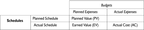
Figure 9-8. Selected earned value measurement metrics.
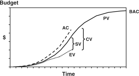
As a project progresses, both PV and AC may be compared with EV. Any difference between AC and EV—in the figure this is shown as CV, or cost variance—must be due to a spending issue, because the metrics are based on the same schedule. Similarly, any difference between PV and EV—SV, or schedule variance on the graph—has to be due to a timing problem. There are indices and other more complex derived metrics for EVM, but all are based on the fundamental three: EV, PV, and AC.
There is much discussion concerning the value of EVM for technical projects. It can represent quite a bit of overhead, and for many types of technical projects, tracking data at the level required by EVM is thought to be overkill. EVM typically can accurately predict project overrun at the point where 15 percent of the project budget is consumed.
If the metrics for EVM seem impractical for your projects, the related alternative of activity closure index (listed with the schedule metrics) provides similar diagnostic information based on the higher granularity of whole activities. This metric provides similar information with a lot less effort. Activity closure rate is less precise, but even it will accurately spot an overrun trend well before the project halfway point.
Retrospective project metrics Retrospective metrics determine how well a process worked after it completes. They are the project environment’s rear-view mirror. Measurement baselines are based on history, and these metrics are most useful for longer-term process improvement. Use retrospective project metrics to:
• Track trends
• Validate methods used for predictive metrics
• Identify recurring sources of risk
• Set standards for reserves (schedule and/or budget)
• Determine empirical expectations for “unknown” project risk
• Decide when to improve or replace current project processes
Retrospective project metrics include:
Scope Risk
• Number of accepted changes
• Number of defects (number, severity)
• Actual “size” of project deliverable analysis (components, lines of noncommented code, system interfaces)
• Performance of deliverables compared to project objectives
• Actual project duration compared to planned schedule
• Number of new unplanned activities
• Number of missed major milestones
• Assessment of duration estimation accuracy
Resource Risk
• Actual project budget compared to planned budget
• Total project effort
• Cumulative overtime
• Assessment of effort estimation accuracy
• Life-cycle effort percentages by project phase
• Added staff
• Staff turnover
• Performance to standard estimates for standardized project activities
• Variances in travel, communications, equipment, outsourcing, or other expense subcategories
Overall Risk
• Late project defect correction effort as a percentage of total effort
• Number of project risks encountered
• Project issues tracked and closed
• Actual measured ROI
Financial Metrics
Project risk extends beyond the normal limits of project management, and project teams must consider and do what they can to manage risks that are not strictly “project management.” There are a number of methods and principles used to develop predictive metrics that relate to the broad concept of ROI, and an understanding of these is essential to many types of technical projects. As discussed in Chapter 3 with market risks, ROI analysis falls only partially within project management’s traditional boundaries. Each of the several ways to measure ROI comes with benefits, drawbacks, and challenges.
The time value of money The foundation of most ROI metrics is the concept of the time value of money. This is the idea that a quantity of money today is worth more than the same quantity of money at some time in the future. How much more depends on a rate of interest (or discount rate) and the amount of time. The formula for this is:
PV = FV/(1 + i)n, where
PV is present value
FV is future value
i is the periodic interest rate
n is the number of periods
If the interest rate is 5 percent per year (.05) and the time is one year, $1 today is equivalent to $1.05 in the future.
Payback analysis Even armed with the time value of money formula, it is rarely easy to determine the worth of any complex investment with precision, and this is especially true for investments in projects. Project analysis involves many (perhaps hundreds) of parameters and values, multiple periods, and possibly several interest rates. Estimating all of this data, particularly the value of the project deliverable after the completion of the project, can be very difficult.
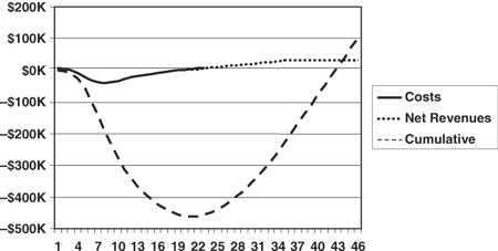
The most basic ROI model for projects is simple payback analysis, which assumes no time value for money (equivalent to an interest rate of zero). This type of ROI metric has many names, including break-even time, payback period, or the “return map.” Payback analysis adds up all expected project expenses and then proceeds to add expected revenues, profits, or accrued benefits, period by period, until the value of the benefits balances the costs. As projects rarely generate benefits before completion, the cumulative financials swing heavily negative, and it takes many periods after the revenues and benefits begin to reach “break-even.”
The project in the graph in Figure 9-9 runs for about five months, with a budget of almost $500,000. It takes another six months, roughly, to generate returns equal to the project’s expenses. Simple payback analysis works fairly well for comparing similar-length projects to find the one (or ones) that recovers its costs most rapidly. It has the advantage of simplicity, using predictive project cost metrics for the expense data and sales or other revenue forecasts for the rest.
Refining simple payback analysis to incorporate interest (or discount) rates is not difficult. The first step is to determine an appropriate interest rate. Some analyses use the prevailing cost of borrowing money, others use a rate of interest available from external investments, and still others use rates based on business targets. The rate of interest selected can make a significant difference when evaluating ROI metrics.
Figure 9-9. Simple payback analysis.
Once an appropriate interest rate is selected, each of the expense and revenue estimates can be discounted back to an equivalent present value before it is summed. The discounted payback or break-even point again occurs when the sum, in this case the cumulative present value, reaches zero. For a nonzero interest rate, the amount of time required for payback will be significantly longer than with the simple analysis, since the farther in the future the revenues are generated, the less they contribute because of the time value of money. Discounted payback analysis is still relatively easy to evaluate, and it is more suitable for comparing projects that have different durations.
Payback analysis, with and without consideration of the time value of money, is often criticized for being too short-term. These metrics determine only the time required to recover the initial investment. They do not consider any benefits that might occur following the break-even point, so a project that breaks even quickly and then generates no further benefits would rank higher than a project that takes longer to return the investment but represents a much longer, larger stream of subsequent revenues or benefits.
Net present value Total net present value (NPV) is another method to measure project ROI. NPV follows the same process as the discounted payback analysis, but it does not stop at the break-even point. NPV includes all the costs and all the anticipated benefits throughout the expected life of the project deliverable. Once all the project costs and returns have been estimated and discounted to the present, the sum represents the total present value for the project. This total NPV can be used to compare possible projects, even projects with very different financial profiles and time scales, based on all expected project benefits.
Total NPV effectively determines the overall expected return for a project, but it tends to favor large projects over smaller ones, without regard to other factors. A related idea for comparing projects normalizes their financial magnitudes by calculating a profitability index (PI). The PI is a ratio, the sum of all the discounted revenues divided by the sum of all the discounted costs. PI is always greater than one for projects that have a positive NPV, and the higher the PI is above one, the more profitable the project is expected to be.
Even though these metrics require additional data—estimates of the revenues or benefits throughout the useful life of the deliverable—they are still relatively easy to evaluate.
Internal rate of return Another way to contrast projects of different sizes is to calculate an internal rate of return (IRR). IRR uses the same estimates for costs and returns required to calculate total net present value, but instead of assuming an interest rate and calculating the present value for the project, IRR sets the present value equal to zero and then solves for the required interest rate. Mathematically, IRR is the most complex ROI metric, as it must be determined using iteration and “trial and error.” For sufficiently complicated cash flows, there may even be several values possible for IRR (this occurs only if there are several reversals of sign in the cash flows, so it rarely happens in project analysis). These days, using a computer (or even a financial calculator) makes determining IRR fairly straightforward, if good estimates for costs and revenues are available. For each project, the interest rate you calculate shows how effective the project is expected to be as an investment.
ROI estimates All of these ROI methods are attempts to determine the “goodness” of financial investments, in this case, projects. Theoretically, any of these methods is an effective way to select a few promising projects out of many possibilities, or to compare projects with other investment opportunities.
Because of their differing assumptions, these methods may generate inconsistent ranking results for a list of potential projects, but this is rarely the biggest issue with ROI metrics. In most cases the more fundamental problem is with input data. Each of these methods generates a precise numeric result for a given project, based on the input data. For many projects, this information comes from two sources that are historically not very reliable: project planning data and sales forecasts. Project planning data can be made more accurate over time using metrics and adjustments for risk, at least in theory. Unfortunately, project ROI calculations are generally made before much planning is done, when the project cost data is still based on vague information or guesswork, or the estimates come from top-down budget goals that are not correlated with planning at all.
Estimates of financial return are an even larger problem. These estimates are not only usually very uncertain (based on sales projections or other speculative forecasts), they are also much larger numbers, so they are more significant in the calculations. For product development projects, in many cases revenue estimates are higher than costs by an order of magnitude or more, so even small estimating errors can result in large ROI variances.
ROI metrics can be very accurate and useful when calculated retrospectively using historical data, long after projects have completed. The predictive value of ROI measures calculated in advance of projects can never be any more trustworthy than the input data, so a great deal of variation can occur.
Panama Canal: Overall Risks (1907)
When John Stevens first arrived in Panama, he found a lack of progress and an even greater lack of enthusiasm. He commented, “There are three diseases in Panama. They are yellow fever, malaria, and cold feet; and the greatest of these is cold feet.” For the first two, he set Dr. William Gorgas to work, and these risks were soon all but eliminated from the project.
For the “cold feet,” Stevens himself provided the cure. His intense planning effort and thorough analysis converted the seemingly impossible into small, realistic steps that showed that the work was feasible; the ways and means for getting the work done were documented and credible. Even though there were still many specific problems and risks on the project, Stevens had demonstrated that the overall project was truly possible. This was quite a turnaround from John Wallace’s belief that the canal venture was a huge mistake.
With Stevens’s plan, nearly every part of the job relied on techniques that were in use elsewhere, and almost all the work required had been done somewhere before. Project funding was guaranteed by the U.S. government. There were thousands of people able, and very willing, to work on the project, so labor was never an issue. The rights and other legal needs were not a problem, especially after Theodore Roosevelt had manipulated the politics in both the United States and in Panama to secure them. What continued to make the canal project exceptional was its enormous scale. As Stevens said, “There is no element of mystery involved, the problem is one of magnitude and not miracles.”
Planning and a credible understanding of overall project risk are what convert the need for magic and miracles (which no one can confidently promise to deliver) into the merely difficult. Projects that are seen as difficult but possible are the ones that succeed; a belief that a project can be completed is an important factor in how hard and how well people work. When it looks as though miracles will be necessary, people tend to give up, and their skepticism may very well make the project impossible.