Chapter 7

Quantifying and Analyzing Activity Risks

“When you know a thing, to hold that you know it,
and when you do not know a thing, to allow that
you do not know it—this is knowledge.”
—CONFUCIUS

Project planning processes serve several purposes, but probably the most important for risk management is to separate the parts of the work that are well understood, and therefore less risky, from the parts that are less well understood. Often, what separates an impossible project from a possible one is isolating the most difficult work early, so it receives the attention and effort it requires. Risk assessment techniques are central to gaining an understanding of what is most uncertain about a project, and they are the foundation for managing risk. The focus of this chapter is analysis and prioritization of the identified project risks. Analysis of overall project risk will be addressed in Chapter 9.

Quantitative and Qualitative Risk Analysis

Risk analysis strives for deeper understanding of potential project problems. Techniques for doing this effectively may provide either qualitative information for prioritizing risks or quantitative risk measures.

Qualitative techniques are easier to apply and generally require less effort. Qualitative risk assessment is often sufficient for rank-ordering risks, allowing you to select the most significant ones to manage using the techniques discussed in Chapter 8.

Quantitative methods strive for greater precision, and they reveal more about each risk. These methods require more work, but quantitative analysis also provides data on the absolute magnitude of the risks and allows you to estimate schedule and/or budget reserves needed for risky projects.

Although the dichotomy between these approaches is explicit in the PMBOK^® Guide, analysis methods fall into a continuum of possibilities. They range from qualitative assessment using a small number of categories, through methods that use progressively more and finer distinctions, to the extreme of determining specific quantitative data for each risk. If the primary goal of risk analysis is to prioritize risks to determine which ones are important enough to warrant further analysis and response, the easiest qualitative assessment methods generally suffice. If you need to assess project-level risk with maximum precision, then you will need quantitative assessment methods (though the nature of the available data usually puts a rather modest limit on your accuracy).

Whatever assessment method you apply, the foundation goes back to the simple formula discussed in Chapter 1: “loss” multiplied by “likelihood.” The realm of likelihood is statistics and probability, topics that many project contributors find daunting and even counterintuitive. Loss in projects is measured in impact: time, money, and other project factors, including some that may be difficult to quantify. These two parameters characterize risk, and evaluating each poses challenges.

Risk Probability

At the beginning of a project, risks are uncertain. The likelihood, or probability, for any specific risk will always be somewhere between zero (no chance of occurrence) and one (inevitable occurrence). Looking backward from the end of a project, every risk has one of these two values; either it happened or it did not. Qualitative risk assessment methods divide the choices into probability ranges and require project team members to assign each risk to one of the defined ranges. Quantitative risk assessment assigns each risk a specific fraction between zero and one (or between zero and 100 percent).

Risk probabilities must all fall within this range, but picking a value between zero and one for a given risk poses difficulties. There are only three ways to estimate probabilities. For some situations, such as flipping coins and throwing dice, you can construct a mathematical model and calculate an expected probability. In other situations, a simple model does not exist, but there may be many historical events that are similar. In these cases statistical analysis of empirical data may be used to estimate probabilities. Analysis such as this is the foundation of the insurance industry. In all other cases, probability estimates are based on guesses. For complex events that seldom or perhaps never occur, you can neither calculate nor measure to determine a probability. Ideas such as referencing analogous situations, scenario analysis, and “gut feel” come into play. For most project risks, probabilities are not based on much objective data, so they are inexact.

We face yet an additional challenge because the human brain does not deal well with probabilities. In most cases there is a strong bias in favor of what we wish to happen. People tend to estimate desirable outcomes as more likely than is justified. (“This lottery ticket is sure to win.”) Conversely, we estimate undesirable outcomes as less likely. (“That risk could never happen.”) Effective risk management requires us to manage this bias, or at least to be wary of it.

Qualitative methods require less precision and do not use specific numerical values. They divide the complete range of possibilities into two or more nonoverlapping probability ranges. The simplest qualitative assessment uses two ranges: “more likely than not (.5 to 1)” and “less likely than not (0 to .4999).” Most project teams are able to select one of these choices for each risk with little difficulty, but the coarse granularity of the analysis makes selecting significant risks for further attention fairly arbitrary.

A more common method for qualitative assessment uses three ranges, assigning a value of high, medium, or low to each risk. The definitions for these categories vary, but these are typical:

• High: 50 percent or higher (likely)

• Medium: Between 10 and 50 percent (unlikely)

• Low: 10 percent or lower (very unlikely)

These three levels of probability are generally easy to determine for project risks without much debate, and the resulting characterization of risk allows you to discriminate adequately between likely and unlikely risks.

Other qualitative methods use four, five, or more categories. These methods tend to use linear ranges for the probabilities: quartiles for four, quintiles for five, and so forth. (The names assigned to five categories could be: Very high, High, Moderate, Low, and Very low.) The more ranges there are, the better the characterization of risk, at least in theory. More ranges do make it harder for the project team to achieve consensus, though.

The logical extension of this continues through increasingly quantitative assessments using integer percentages (100 categories) to continuous estimates allowing fractional percentages. Although the apparent precision improves, the process for determining numerical probabilities can require a lot of overhead, and you must remember that the probability estimates are often based on guesses. The illusion of precision can be a source of risk in itself; making subjective information look objective and precise can result in unwarranted confidence and poor decisions.

Depending on the project, the quality of data available, and the planned uses of the risk data, there are a number of ways to estimate probability. For qualitative assessment methods using five or fewer categories, experience, polling, interviewing, and rough analysis of the risk situation may be sufficient. For quantitative methods, a solid base of historical performance data is the best source, as it provides an empirical foundation for probability assessment and is less prone to bias. Estimating probabilities using methods such as the Delphi technique (mentioned in Chapter 4) or computer modeling (discussed later in this chapter) and employing knowledgeable experts (who may have access to more data than you do) can also potentially improve the quality of quantitative probabilities.

Measurement-based probabilities, when available, serve an additional purpose in project risk management: trend analysis. In hardware projects, statistics for component failure support decisions to retain or replace suppliers for future projects. If custom circuit boards, specialized integrated circuits, or other hardware components are routinely required on projects, quarter-by-quarter or year-by-year data across a number of projects will provide the fraction of components that are not accepted, and provide data on whether process changes are warranted to improve the yields and success rates. Managing risk over the long term relies heavily on metrics, which are discussed in Chapter 9.

Risk Impact

The loss, or project impact, for an individual risk is not as easily defined as the probability. Although the minimum is again zero, both the units and the maximum value are specific to the risk. The impact of a given risk may be relatively easy to ascertain and have a single, predictable value, or it may be best expressed as a distribution or histogram of possibilities. Qualitative risk assessment methods for impact again divide the choices into ranges. The project team assigns each risk to one of the ranges, based on the magnitude of the risk consequences. For quantitative risk assessment, impact may be estimated using units such as days of project slip, money, or some other suitable measure.

Qualitative impact assessment assigns each risk to one of two or more nonoverlapping options that include all the possible risk consequences. A two-option version uses categories such as “low severity” and “high severity,” with suitable definitions of these terms related to attaining the project objective. As with probability analysis, the usefulness of only two categories is limited.

There will be better discrimination using three ranges, where each risk is assigned a value of high, medium, or low. The definitions for these categories vary, but commonly they relate to the project objective and plan as follows:

• High: Project objective is at risk (mandatory change to one or more of scope, schedule, or resources).

• Medium: Project objectives can be met, but significant replanning is required.

• Low: No major plan changes; the risk is an inconvenience or it will be handled through overtime or other minor adjustments.

These three levels of project impact are not difficult to assess for most risks and provide useful data for sequencing risks according to severity.

Other methods use additional categories, and some partition impact further into specific project factors, related to schedule, cost, and scope and other factors. Impact measurement is open-ended; there is no theoretical maximum for any of these parameters (in a literally impossible project, both time and cost may be considered infinite). Because the scale is not bounded, the categories used for impact are often geometric, with small ranges at the low end and progressively larger ranges for the upper categories. For an impact assessment using five categories, definitions might be:

1. Very low: Less than 1 percent impact on scope, schedule, cost, or quality

2. Low: Less than 5 percent impact on scope, schedule, cost, or quality

3. Moderate: Less than 10 percent impact on scope, schedule, cost, or quality

4. High: Less than 20 percent impact on scope, schedule, cost, or quality

5. Very high: 20 percent or more impact on scope, schedule, cost, or quality

Risks are assigned to one of these categories based on the most significant predicted variance, so a risk that represents a 10 percent schedule slip and negligible change to other project parameters would be categorized as “moderate.” As with probability assessment, the more ranges there are, the better the characterization of risk, but the harder it is to achieve agreement among the project team.

Similar assessment may also be devised to look at specific kinds of risk separately, such as cost risk or schedule risk, to determine which are most likely to affect the highest project priorities.

The most precise assessment of impact requires quantitative estimates for each risk. Few risks relate only to a single aspect of the project, so there may be a collection of measurement estimates, generally including at least cost and schedule impact. Cost is conceptually the simplest, because it is unambiguously measured in dollars, yen, euros, or some other easily described unit, and any adverse variance will directly affect the project budget. Schedule impact is not as simple, because not every activity duration slippage will necessarily represent an impact to the schedule. Activities off the critical path will generate schedule impact only for adverse variances that exceed the available float. As with other project estimating, determining cost and schedule variances attributable to risks is neither easy nor necessarily accurate. Quantitative assessments of risk impact may look precise, but the accuracy of such estimates is often questionable.

The discussion of risk impact here so far has focused on measurable project information—even the qualitative categories tend to be based on numerical ranges. Limiting impact assessment to such factors overlooks risk impact that may be difficult to quantify. For some risks such an approach may ignore factors that may well be the most significant. Because the impact resulting from these other factors can be hard to determine with precision, it is generally ignored or assumed to be insignificant in project risk assessment. Categories for these more “qualitative” types of impact, listed in sequence from the most narrow perspective to the broadest, include:

• Personal consequences

• Career penalties

• Loss of team productivity

• Team discord

• Organizational impact

• Business and financial consequences

Measurable consequences for some of these factors may be roughly quantified, at least in the short term. Such analysis, however, may vastly underestimate true long-term overall effects. For other factors, it may seem impossible to incorporate these consequences in a way that permits straightforward assessment. Despite the challenges, it is worthwhile to list and carefully consider the potential consequences of these factors, because the true overall impact for many project risks may well be dominated by them. More detail follows, along with some suggestions about how to integrate these factors into your risk assessment. Although not exhaustive, the lists that follow should provide food for thought.

Many risks faced by projects include potential personal consequences that can be quite severe, ranging from inconveniences and aggravations to major impositions. These include:

• Marital problems, divorce, and personal relationship troubles

• Cancelled vacations

• Missed family activities

• Excessive unpaid overtime

• Fatigue and exhaustion

• Deterioration of health

• Exposure to unsafe conditions, poisonous or volatile chemicals, dangerous environments, or undesirable modes of travel

• Loss of face, embarrassment, lowered prestige, bruised egos, and reduced self-esteem

• Required apologies and “groveling”

Major project difficulties can lead to a variety of career penalties, and personal reputations may suffer, leading to:

• Job loss

• Lowered job security

• A bad performance appraisal

• Demotion

• No prospect for promotion

Both during and following a major risk, team members may work less efficiently. Loss of team productivity may result from:

• More meetings

• Burnout

• Increased communication overhead, especially if across multiple time zones

• Added stress, tension, pressure

• More errors, inaccuracies

• Chaos, confusion

• Rework

• Additional reporting, reviews, interruptions

• Individuals assuming responsibility for work assigned to others

• Exhaustion of project reserves, contingency

Even if productivity is unaffected, team discord may rise. The success of a project relies on maintaining good teamwork among your project contributors. When things start to unravel, the consequences can include:

• Conflict, hostility, resentment, and short tempers

• Lack of cooperation and strained relationships

• Low morale

• Frustration, disappointment, and discouragement

• Demoralization and disgruntlement

Project risk consequences may lead to organizational impact that extends well beyond your current project’s prospects for success. Some of these include:

• Delayed concurrent projects

• Late starts for following projects

• Resignations and staff turnover

• Loss of sponsor (and stakeholder) confidence, trust, and goodwill

• Questioning of methods and processes

• Ruined team reputations

• Micromanagement and mistrust by supervisors

• Required escalations and expediting of work

• The need to get lawyers involved

Finally, some risks will have significant business and financial consequences. Although these effects may well be estimated and quantified, the true impact is generally measurable only after—and often well after—the project is closed. Some examples are:

• Loss of business to competitors and competitive disadvantage

• Bad press, poor public relations, and loss of organizational reputation

• Customer dissatisfaction and unhappy clients

• Loss of future business and lowered revenues

• Reduced margins and profits

• Loss of client trust, confidence

• Complications resulting from failure to meet legal, regulatory, industry standards, or other compliance requirements

• Damaged partner relationships

• Reduced performance of the project deliverable

• Compromised quality or reliability

• Rushed, inadequate testing

• Missed windows of opportunity

• Continued cost of obsolete systems or facilities

• Inefficient, unpleasant manual workarounds

• Service outages and missed service level agreements

• Bankruptcy and business failure (if the project is big enough)

Although for some risks the short-term quantifiable impact on your project’s schedule or budget may be modest, the overall consequences, particularly some of the items on the last two lists, will have major impact on the organization. Even though these potential impacts may be primarily qualitative, it is desirable to integrate them into your risk assessment and prioritization. One way to do this is to apply impact criteria such as in the five-level assessment demonstrated in the following table.

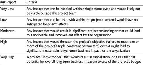
Analysis based on these criteria remains subjective, but it provides a practical way to assess the relative importance of project risks—even risks where measurable impact is difficult to pin down.

Qualitative impact assessment using three to five categories is usually relatively easy, and it is sufficient for prioritizing risks based on severity. Techniques such as polling, interviewing, team discussion, and reviews of planning data are effective for assigning risks to impact categories. As with probability assessment for each risk, the best foundation for quantitative estimates of impact is history, along with techniques such as Delphi, computer modeling, and consulting peers and experts.

For quantitative assessments of impact in situations that frequently repeat, statistics may be available. A good way to provide credible quantitative impact data is to select the mean of the distribution for initial estimates of duration or cost and use the difference between that estimate and the measured “90 percent” point. This principle is the basis for Program Evaluation and Review Technique (PERT) analysis. The PERT estimating technique was discussed in Chapter 4, and other aspects of PERT and related techniques are covered later in this chapter and in Chapter 9.

Qualitative Risk Assessment

The minimum requirement for risk assessment is a sequenced list of risks, rank-ordered by perceived severity. You can sort the listed risks from most to least significant using your assessment of loss times likelihood. If your list of risks is short enough, you can quickly arrange the list based on few passes of pair-wise comparisons, switching any adjacent risks where the more severe of the two is lower on the list. The most serious risks will bubble to the top and the more trivial ones will sink to the bottom. This technique is generally done by a single individual.

A similar technique, related to Delphi, combines data from lists sorted individually by each member of a team. The risks on each list are assigned a score equal to their position on the list, and all the scores for each risk are summed. The risk with the lowest total score heads the composite list, and the rest of the list is sorted based on the aggregate scores. If there are significant variances in some of the lists, further discussion and an additional iteration may lead to better consensus. The resulting list will be more objective than a sequence created by an individual, and it represents the whole team.

Although these sorting techniques result in an ordered risk list, such a list shows only relative risk severity, without indication of the project exposure that each risk represents.

Risk Assessment Tables

Qualitative risk assessment based on categorization of both probability and impact provides greater insight into the absolute risk severity. A risk assessment table or spreadsheet where risks are listed with category assignments for both probability and impact, as in Figure 7-1, is one approach for this.

After listing each risk, assign a qualitative rating (such as High/Moderate/Low) for both probability and impact. Consider all potential impact, not just that which is easily measured, and be skeptical about probabilities. Fill in the last column, “Overall Risk,” based on “loss times likelihood.” Although any number of rating categories may be used, the quickest method that results in a meaningful sort uses three categories (defined as in the earlier discussions of probability and impact) and assigns either combinations of the categories or weights such as 1, 3, and 9 for low, moderate, and high, respectively. An example of a sorted qualitative assessment for five risks might look like Figure 7-2.

For the data in the last column, categories may be combined (as shown), factors multiplied (the numbers would be 27, 9, 9, 3, and 1), or “stoplight” icons displayed to indicate risk (red for high, yellow for moderate, and green for low). From a table such as Figure 7-2, you can select risks above a certain level, such as moderate, for further attention.

Figure 7-1. Risk assessment table.

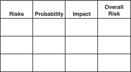
Figure 7-2. Qualitative risk assessment example.

Risk Assessment Matrices

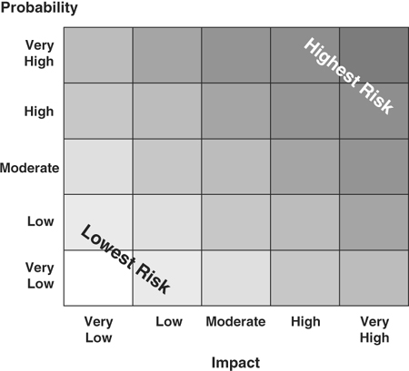
An alternative method for qualitative risk assessment involves placing risks on a two-dimensional matrix, where the rows and columns represent the categories of probability and impact. The matrices may be two-by-two, three-by-three, or larger. Risk matrices are generally square, but they may have different numbers of categories for probability and impact. Figure 7-3 is an example of a five-by-five matrix.

The farther up and to the right a risk is assessed to be, the higher its overall assessment. Risks are selected for management based on whether the cell in the matrix represents a risk above some predetermined level of severity. An organization’s risk tolerance (or appetite) is generally bounded by one of the sets of lighter gray cells in the matrix.

A matrix such as Figure 7-3 is usually applied to the analysis of risks having negative consequences (threats). It may also be used to assess uncertain project opportunities. Some of the opportunities discussed in Chapter 6 relate to scoping choices and planning decisions, where the only uncertainty is whether an opportunity is adopted as part of the project or not. Other opportunities, like most risks, hinge on circumstances that might or might not happen. For these opportunities assessment is based on likelihood and (instead of loss) gain. An example of this type of opportunity might be buying something needed by the project that occasionally goes on sale. Once the opportunity to purchase the item at a reduced price is recognized, managing this “risk” might involve delaying the purchase to potentially take advantage of a better price. For most projects, there are far fewer opportunities of this sort than there are risks.

Figure 7-3. Risk assessment matrix.

For analysis of uncertain opportunities, the definition of probability is unchanged. The impact is also similar, but for opportunities the categories relate to beneficial variances, not harmful ones. Using the same matrix, you can assess potentially positive events to determine those that deserve further attention—again by focusing near the corner representing the combination of highest impact and probability. Another variant on this matrix technique joins together the threat matrix and a mirror-image opportunity matrix into a single matrix (for this case, five cells high and ten cells wide). You find the highest impact in the middle using the combined matrix, so the uncertain events most deserving your attention will be those in the cells near the top and center of the matrix.

Assessing Options

Standard project network charts do not generally permit the use of conditional branching. Because it is not uncommon to have places in a project schedule where one of several possible alternatives, outcomes, or decisions will be chosen, you need some method for analyzing the situation. One qualitative way around this limitation is to construct a baseline plan using the assumption that seems most likely and deal with the other possible outcomes as risks. If it is not possible to determine which outcome may be most likely, a prudent risk manager will usually select the one with the longest duration (or highest cost) to include in the project baseline, but any one option may be selected. Assessing the risk associated with choosing incorrectly involves determining the estimated impact on the project if a different option is picked, weighted by the probability of this happening (loss times likelihood once again). List the significant ones on your risk register and sort them with your other project risks.

Data Quality Assessment

Not all risks are equally well understood. Some risks happen regularly, and data concerning them is plentiful. Other project risks arise from work that is unique compared with past projects. Assessment of probability and impact for these risks tends to be based on inadequate information, so it’s common to underestimate overall risk.

Even with qualitative risk assessment, these poorly understood risks can be identified and singled out for special treatment. For each assessment, consider the quality, reliability, and integrity of the data used to categorize probability and impact. Where the information seems weak, seek out experts or other sources of better information. You can also err on the side of caution and bump up your probability and impact estimates to elevate the visibility of the risk.

Other Factors

Although a risk that has high probability and impact will require your attention, those that relate to work well into the future may not need it immediately. Other aspects of risk that may enter into qualitative assessment are urgency and surprise. The impact of even a modest risk can cause harm to your project overall if it happens early and affects the perception of your competence or the teamwork of your contributors. Risks tend to cascade, so early problems may lead to more trouble later in the project. If a risk relates to work that is imminent, factor this into your impact assessment, increasing it where justified.

Similarly, some risks are relatively easy to see coming. Other risks, such as the damaging example from the PERIL database of receiving a late deliverable from an outsourcing partner, are hard to detect in advance. Consider the trigger events for each risk when estimating impact, and increase it for risks where the harm may be amplified by the surprise factor.

Risks Requiring Further Attention

The main objective of qualitative risk assessment is to identify the major risks by prioritizing the known project risks and rank-ordering them from most significant to least. The sequenced list may be assembled using any of the methods described, but the use of three categories (low, moderate, and high) for both probability and impact generally provides a good balance of adequate analysis and minimal effort and debate. However you analyze and sort the list, you need to partition the risks that deserve further consideration from risks that seem too minor to warrant a planned response.

The first several risks on your prioritized list nearly always require attention, but the question of how far down the list to go is not necessarily simple. One idea is to read down the list, focusing on the consequences and the likelihood of each risk until you reach the first one that won’t keep you awake at night. The “gut feel” test is not a bad way to select the boundary for a sorted risk list. A similar idea using consensus has team members individually select the cut-off point, and then discuss as a team where the line should be, based on individual and group experiences. You can also set an absolute limit, such as moderate overall risk, or you can use a diagonal stair-step boundary from the upper left to the lower right in a matrix. Whatever method you choose, review each of the risks that are not selected to ensure that there are none below the line that warrant a response.

Following this examination, you are ready to prepare an abridged list of risks for potential further quantitative analysis and management.

Quantitative Risk Assessment

As stated earlier in the chapter, quantitative risk assessment involves more effort than qualitative techniques, so qualitative methods are generally used for initial risk sorting and selection. This is not absolutely necessary, though, because each of the qualitative methods discussed has a quantitative analogue that could be used to sequence the risk list. Qualitative tables have their categories for probability and impact replaced by absolute numerical estimates. The cells in risk matrices are transformed into continuous two-dimensional graphs for plotting the estimates. Quantitative techniques such as sensitivity analysis, more rigorous statistical methods, decision trees, and simulations can provide further insight into project risk, and may also be used for overall project risk assessment.

Sensitivity Analysis

Not all risks are equally damaging. Schedule impact not affecting resources is significant only when the estimated slippage exceeds any available float. For simple projects, a quick inspection of the plan using the risk list will distinguish the risks that are likely to cause the most damage. For more complex networks of activities, using a copy of the project database that has been entered into a scheduling tool is a fast way to detect risks (and combinations of risks) that are most likely to result in project delay. Schedule “what if” analysis uses worst-case estimates to investigate the overall project impact for each risk. By sequentially entering your scheduling data and then backing it out, you can determine the quantitative schedule sensitivity for each schedule risk.

Unlike activity slippage, all adverse cost variances contribute to budget overruns. However, for some projects not all cost impact is accounted for in the same way. If a risk results in an out-of-pocket expense for the project, then it impacts the budget directly. If the cost impact involves a capital purchase, then the project impact may be only a portion of the actual cost, and in some cases the entire expense may be accounted for elsewhere. An increase in overhead cost, such as a conference room commandeered as a “war room” for a troubled project, is seldom charged back to the project directly. Increased costs for communications, duplication, shipping, and other services considered routine are frequently not borne directly by technical projects. Travel costs in some cases may also not be allocated directly. Although it is generally true that all cost and other resource impact is proportionate to the magnitude of the variance, it may be worthwhile to segregate potential direct cost variances from any that are indirect.

Quantitative Risk Assessment Tables

For quantitative assessment, the same sort of table or spreadsheet discussed previously can be filled in with numerical probabilities instead of the categories used for qualitative assessment. For each risk, estimate the impact in cost, effort, time (but only time in excess of any available scheduling flexibility), or other factors, and then assess overall risk as the product of the impact estimates and the selected probability. One drawback of using this method for sequencing risks is that for some risks it may be difficult to develop precise consensus for both the impact and probability. A second, more serious issue is that impact may be measured in more than one way (as examples, time and money), making it difficult to ascertain a single uniform quantitative assessment of overall risk.

Although you could certainly list impacts of various kinds, weighted using the estimated probabilities, you may find that sorting based on this data is not straightforward. This can be overcome by selecting one type of impact, such as time, and converting impact of other kinds into an equivalent project duration slip (as was done in the PERIL database). You could also develop several tables, one for cost, another for schedule, and others for scope, quality, safety, or any other type of impact for which you can develop meaningful numerical estimates. You can then sort each table on a consistent basis, and select risks from each for further attention. This multiple-table process also requires you to do a final check to detect any risks that are significant only when all factors are considered together.

Two-Dimensional Quantitative Analysis

The qualitative matrix converts to a quantitative tool by replacing the rows and columns with perpendicular axes. Probability may be plotted on the horizontal axis from zero to 100 percent, and impact may be plotted on the vertical axis. Each risk identified represents a point in the two-dimensional space, and risks requiring further attention will be found again in the upper right, beyond a boundary defined as “risky.” As with tables, this method is most useful when all risks can be normalized to some meaningful single measure of impact such as cost or time.

A variation on this concept plots risks on a pair of axes that represent estimated project cost and project schedule variances, representing each risk using a “bubble” that is sized proportionately with estimated probability instead of a single point. Because impact is higher for bubbles farther from the origin, several boundaries are defined for the graph. A diagonal close to the origin defines significant risk for the large (very likely) bubbles, and other diagonals farther out define significant exposure for the smaller bubbles. In Figure 7-4, there are several risks that are clearly significant. Risk F has the highest impact, and Risk E is, well, risky. Others would be selected based on their positions relative to the boundaries of the graph.

PERT

PERT methodology, discussed earlier, has assumed a number of meanings. The most common, which actually has little to do with PERT methodology, is associated with the graphical network of activities used for project planning, often referred to as a PERT chart. Logical project networks are used for PERT analysis, but PERT methodology went beyond the deterministic, single-point estimates of duration to which “PERT charts” are generally limited. A second, slightly less common meaning for PERT relates to three-point estimating, which was discussed with identifying schedule risk in Chapter 4. The original purpose of PERT was actually much broader.

Figure 7-4. Risk assessment graph.

The principal reason PERT was originally developed in the late 1950s was to help the U.S. military quantitatively manage risk for large defense projects. PERT was used on the development of the Polaris missile systems, on the NASA manned space projects, including the Apollo moon missions, and on countless other government projects. The motivation behind all of this was the observation that as programs became larger, they were more likely to be late and to have significant cost overruns. PERT was created to provide a better basis for setting expectations on these massive, expensive endeavors.

PERT is a specific example of quantitative risk analysis, and it is applied to both schedule (PERT Time) and budget (PERT Cost) exposures. PERT is based on some statistical assumptions about the project plan, requiring both estimates of likely outcomes and estimates of the uncertainty for these outcomes. PERT techniques may be used to analyze all project activities or only those activities that represent high perceived risk. In either case, the purpose of PERT was to provide data on overall project risk. This application of PERT methodology is covered in Chapter 9.

PERT Time was mentioned in Chapter 4, using three estimates for each activity—an optimistic estimate, a most likely estimate, and a pessimistic estimate—to calculate an “expected estimate.” PERT Cost also uses three estimates to derive an expected activity cost, using essentially the same formula:

c_e = (c_o + 4c_m + c_p)/6, where
c_e is the “expected” cost
c_o is the “optimistic” (lowest realistic) cost
c_m is the “most likely” cost
c_p is the “pessimistic” (highest realistic) cost

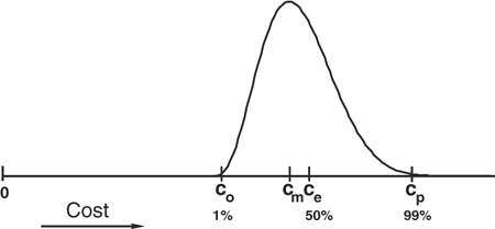
As with PERT Time, the standard deviation is estimated to be (c_p – c_o)/6. A distribution showing this graphically is in Figure 7-5.

PERT Cost estimates are generally done in monetary units (pesos, rupees, euros), but they may also be evaluated in effort (person-hours, engineer-days) instead of, or in addition to, the financial estimates.

Whether for time or cost, PERT ideas are useful in gathering risk information about project activities, particularly concerning the pessimistic (or worst-case) estimates as discussed in Chapter 4. PERT also provided the basis for simulation-based project analysis techniques that are better able to account for schedule fan-in risks and correlation factors. Project simulations are referenced later in this chapter and explored in more detail in Chapter 9.

Figure 7-5. Cost estimates for PERT analysis.

Statistical Concepts and Probability Distributions

Risk impact discussed so far has been based primarily on single-point, deterministic estimates. PERT, as originally defined, assumed a continuum of possibilities. PERT used three-point estimates to define a Beta distribution, a bell-shaped probability density function that can skew to the right or left. Figure 7-5 is an example of a Beta distribution fitted to three estimates for activity cost. This example uses the traditional “1 percent tails” to bound the range of possibilities, but other variants are based on 5 or 10 percent tails.

Probability distribution functions, or even discrete data values defined by a histogram, may better describe the range of potential impact for a given risk. Some additional distributions that are used include:

• Triangular (a linear rise from optimistic estimate to the most likely, followed by a linear decline to the pessimistic estimate)

• Normal (the Gaussian bell-shaped curve, with the most likely and expected values half-way between the extremes)

• Uniform (all values in the range are assumed equally likely, also with the most likely and expected values both at the midpoint)

There are many other more exotic distributions available, along with limitless histograms that are possible. The precise shape of the distribution turns out to be relatively unimportant, though, because it has only a small effect on the two parameters that matter the most for risk analysis: the mean and the standard deviation of the distribution. Assessment of risk really only requires these two parameters, and they vary little, regardless of the distribution you chose. In addition, although it is theoretically possible to carry out a detailed risk analysis mathematically, it is impractical. Project risk analysis using probability distributions is most commonly done by computer simulation or by rough manual methods to approximate the results. The choice of a precise distribution for each activity has minimal effect on quantitative assessment of risk for most projects.

For those who may be interested, some examples follow that show why the choice of a probability density function for the estimates is not terribly crucial. (If you do not need convincing of this, just note that any approach that you find easy to work with can produce useful quantitative risk data, and skip ahead to the discussion of range estimating.)

The original PERT formulation assumed that the three estimates defined a continuum shaped as a Beta distribution. The precise shape of the distribution defined by the three estimates does not have much effect on the resulting analysis. Even using only two estimates “most likely” and “worst-case,” as discussed in Chapter 4, provides useful risk information. These examples all use estimates of 15 and 21 days as limits for the duration estimate ranges.

For Figure 7-6, the optimistic estimate has been assumed identical to the most likely. When values are plugged into the formula to calculate the expected duration, the PERT formula results in a t_e of 16 days.

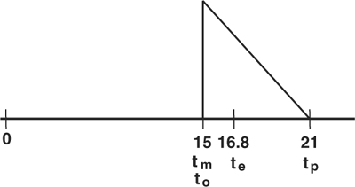
A similar result, mathematically much simpler, can be estimated using a triangular distribution, as in Figure 7-7.

For a triangular distribution, the point at which the areas to the right and left are equal occurs slightly less than 30 percent of the way along the triangle’s base. Using the same estimates as before for t_o, t_m, and t_p, the estimate for t_e is just under 16.8 days.

Symmetric distributions increase the expected estimate a bit more. Using a normal distribution (Figure 7-8) or a simple uniform distribution (Figure 7-9) for the probability distribution that lies between the range limits results in an expected value for this example of 18 days. (A symmetric triangular distribution would be equivalent to these.)

The weighted-average PERT formula for the Beta distribution in Figure 7-5 estimates t_e at 16 days, and all the other examples evaluate it to be a bit higher. For a quantitative risk assessment, some value above the mean will be selected to represent impact (a 90 percent point is common). Although these points are also not identical for the various distributions, they all are quite close together, near the upper (t_p) estimate. Risk assessment is related to the variance for the chosen distribution, which for these examples will all be similar because in each case, the ranges are the same.

Figure 7-6. Two-estimate Beta distribution.

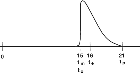
Figure 7-7. Triangular distribution.

If t_p is 21 days, the 90 percent point for each of these distributions is about 20 days (rounded off to the nearest whole day), regardless of the distribution selected. There are many tools and techniques capable of calculating all of this with very high precision, displaying many (seemingly) significant digits in the results. Considering the precision and expected accuracy of the input data, though, the results are at best accurate only to the nearest whole day. Arguments over the “best” distribution to use and endless fretting over how to proceed are not a good investment of your time. Almost any reasonable choice of distribution will result in comparable and useful results for risk analysis, so use the choice that is easiest for you to implement.

Figure 7-8. Normal distribution.

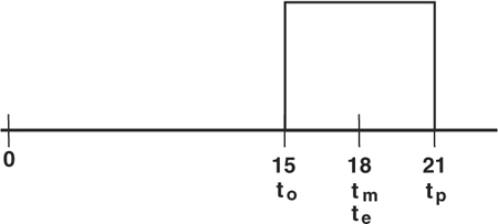
Figure 7-9. Uniform distribution.

At the project level, where PERT data for all the activities is combined, the distributions chosen for each activity become even more irrelevant. The larger the project, the more the overall analysis for project cost and duration tends to approximate a normal bell-shaped curve (more on this in Chapter 9).

Setting Estimate Ranges

What does matter a great deal for risk assessment is the range specified for the estimates. Setting the range to be too narrow (which is a common bias) will materially diminish the quantitative perception of risk. Risk, assessed using PERT or similar techniques, is based on the total expected variation in possible outcomes, which varies directly with the size of the estimate range.

Arriving at credible upper and lower limits for cost and duration estimates is difficult. One way to develop this data is through further analysis of potential root causes of each activity that has substantial perceived risk. As discussed in Chapter 4, seeking worst-case scenarios is the most powerful tool for estimating the upper limits. Be realistic about potential consequences; it’s easy to minimize or overlook the potential impact of risks.

When there is sufficient historical information available, the limits (and possibly even the shape) of the distribution may be inferred from the data. Discussions and interviews with experts, project stakeholders, and contributors may also provide information useful in setting credible range boundaries.

In any event, quantitative assessment of risk impact depends on credible three-point (or at least expected and worst-case) project estimates. Project-level risk assessment using PERT methodology and related techniques will be explored in detail in Chapter 9.

Decision Trees

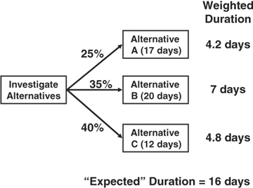
When only a small number of options or potential outcomes are possible, decision trees may also be useful for quantitative risk assessment. Decision tree analysis is a quantitative version of the process for assessing options discussed earlier in this chapter with qualitative assessment techniques. Decision trees are generally used to evaluate alternatives prior to selecting one of them to execute. The concept is applied to risk analysis in a project by using the weights and estimates to ascertain potential impact for specific alternatives.

Whenever there are points in the project where several options are possible, each can be planned and assigned a probability (the sum for all options totaling 100 percent). As with PERT, an “expected” estimate for either duration or cost may be derived by weighting the estimates for each option and summing these figures to get a “blended” result. Based on the data in Figure 7-10, a project plan containing a generic activity (that could be any of the three options) with an estimate of 16 days would result in a more realistic plan than simply using the 12-day estimate of the “most likely” option. The schedule exposure of the risk situation here may be estimated by noting the maximum adverse variance (an additional four days, if the activity is schedule critical) and associating this with an expected probability of 35 percent. (Another option for this case would be to assume the worst and schedule 20 days, treating the other possibilities as opportunities to be managed.)

Figure 7-10. Decision tree for duration.

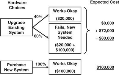
Decision analysis may also be used to guide project choices that are based on costs. You can use decision trees to evaluate expected monetary value for various options. The analysis can explore alternatives that have the lowest expected cost and those with the lowest expected cost variance. Decision analysis can help in minimizing project risks whenever there are several alternatives, such as upgrading existing equipment versus purchasing new hardware. The analysis of costs in Figure 7-11 argues for replacement to minimize cost variance (none, instead of the $20,000 to $120,000 associated with upgrade), and for upgrade to minimize the expected cost. As is usual on projects, there is a trade-off between minimizing project parameters and minimizing risk—you must decide which is more important and balance the decisions with your eyes open.

Simulation and Modeling

Decision trees are useful for situations where you have discrete estimates. In more complex cases, options may be modeled or simulated using Monte Carlo or other computer techniques. If the range of possibilities for an activity’s duration or cost are assumed to be a statistical distribution, the standard deviation (or variance) of the distribution is a measure of risk. The larger the range selected for the distribution, the higher the risk for that activity. For single activities, modeling with a computer is rarely necessary, but when several activities are considered together (or the project as a whole), computer-based simulations are useful and effective. Use of both software tools and manual approximations for this are key topics in Chapter 9.

Figure 7-11. Decision tree for cost.

Panama Canal: Risks (1906–1914)

As with any project of the canal’s size and duration, risks were everywhere. Based on assessment of cost and probability, the most severe were diseases, mud slides, the constant use of explosives, and the technical challenges of constructing the locks.

Diseases were less of a problem on the U.S. project, but health remained a concern. Both of the first two managers cited tropical disease among their reasons for resigning from the project. Life in the tropics in the early 1900s was neither comfortable nor safe. The enormous death toll from the earlier project made this exposure a top priority.

Mud slides were common for both the French and the U.S. projects, as the soil of Panama is not stable, and earthquakes made things worse. Whenever the sloping sides of the cut collapsed, there was danger to the working crews and potential serious damage to the digging and railroad equipment. In addition to this, it was demoralizing to face the repair and rework following the each slide, and the predicted additional effort required to excavate repeatedly in the same location multiplied the cost of construction. This risk affected both schedule and budget; despite precautions, major setbacks were frequent.

Explosives were in use everywhere. In the Culebra Cut, massive boulders were common, and workers set off dynamite charges to reduce them to movable pieces. The planned transit for ships through the man-made lakes was a rain forest filled with large, old trees, and these, too, had to be removed with explosives. In the tropics especially, the dynamite of that era was not stable. It exploded in storage, in transit to the work sites, while being set in place for use, and in many other unintended situations. The probability of premature detonation was high, and the risk to human life was extreme.

Beyond these daunting risks, the largest technical challenge on the project was the locks. They were gigantic mechanisms, among the largest and most complex construction ever attempted. Although locks had been used on canals for a long time, virtually all of them had been built for smaller boats navigating freshwater rivers and lakes. Locks had never before been constructed for large ocean-going ships. (The canal at Suez has no locks; as with the original plan for Panama, it is entirely at sea level.) The doors for the locks were to be huge, and therefore heavy. The volume of water held by the locks when filled was so great that the pressure on the doors would be immense, and the precision required for the seams where the doors closed to hold in the water was also unprecedented for man-made objects so large. The locks would be enormous boxes with sides and bottoms formed of concrete, which also was a challenge, particularly in an earthquake zone. For all this, the biggest technological hurdle was the requirement that all operations be electric. Because earlier canals were much smaller, usually the lock doors were cranked open and shut and the boats were pulled in and out by animals. (To this day, the trains used to guide ships into and out of the locks at Panama are called “electric mules.”) The design, implementation, and control of a canal using the new technology of electric power—and the hydroelectric installations required to supply enough electricity—all involved emerging, poorly understood technology. Without the locks, the canal would be useless, and the risks associated with resolving all of these technical problems were large.

These severe risks were but a few of the many challenges faced on the canal project, but each was singled out for substantial continuing attention. In Chapter 8 on tactics for dealing with risk, we will explore what was done to manage these challenges.