14
PARAMETER ESTIMATION WITH PRIOR PROBABILITIES

In the previous chapter, we looked at using some important mathematical tools to estimate the conversion rate for blog visitors subscribing to an email list. However, we haven’t yet covered one of the most important parts of parameter estimation: using our existing beliefs about a problem.
In this chapter, you’ll see how we can use our prior probabilities, combined with observed data, to come up with a better estimate that blends existing knowledge with the data we’ve collected.
Predicting Email Conversion Rates
To understand how the beta distribution changes as we gain information, let’s look at another conversion rate. In this example, we’ll try to figure out the rate at which your subscribers click a given link once they’ve opened an email from you. Most companies that provide email list management services tell you, in real time, how many people have opened an email and clicked the link.
Our data so far tells us that of the first five people that open an email, two of them click the link. Figure 14-1 shows our beta distribution for this data.
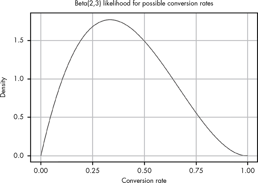
Figure 14-1: The beta distribution for our observations so far
Figure 14-1 shows Beta(2,3). We used these numbers because two people clicked and three did not click. Unlike in the previous chapter, where we had a pretty narrow spike in possible values, here we have a huge range of possible values for the true conversion rate because we have very little information to work with. Figure 14-2 shows the CDF for this data, to help us more easily reason about these probabilities.
The 95 percent confidence interval (i.e., a 95 percent chance that our true conversion rate is somewhere in that range) is marked to make it easier to see. At this point our data tells us that the true conversion rate could be anything between 0.05 and 0.8! This is a reflection of how little information we’ve actually acquired so far. Given that we’ve had two conversions, we know the true rate can’t be 0, and since we’ve had three non-conversions, we also know it can’t be 1. Almost everything else is fair game.
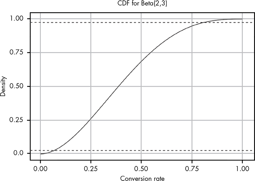
Figure 14-2: CDF for our observation
Taking in Wider Context with Priors
But wait a second—you may be new to email lists, but an 80 percent click-through rate sounds pretty unlikely. I subscribe to plenty of lists, but I definitely don’t click through to the content 80 percent of the time that I open the email. Taking that 80 percent rate at face value seems naive when I consider my own behavior.
As it turns out, your email service provider thinks it’s suspicious too. Let’s look at some wider context. For blogs listed in the same category as yours, the provider’s data claims that on average only 2.4 percent of people who open emails click through to the content.
In Chapter 9, you learned how we could use past information to modify our belief that Han Solo can successfully navigate an asteroid field. Our data tells us one thing, but our background information tells us another. As you know by now, in Bayesian terms the data we have observed is our likelihood, and the external context information—in this case from our personal experience and our email service—is our prior probability. Our challenge now is to figure out how to model our prior. Luckily, unlike the case with Han Solo, we actually have some data here to help us.
The conversion rate of 2.4 percent from your email provider gives us a starting point: now we know we want a beta distribution whose mean is roughly 0.024. (The mean of a beta distribution is α / (α + β).) However, this still leaves us with a range of possible options: Beta(1,41), Beta(2,80), Beta(5,200), Beta(24,976), and so on. So which should we use? Let’s plot some of these out and see what they look like (Figure 14-3).
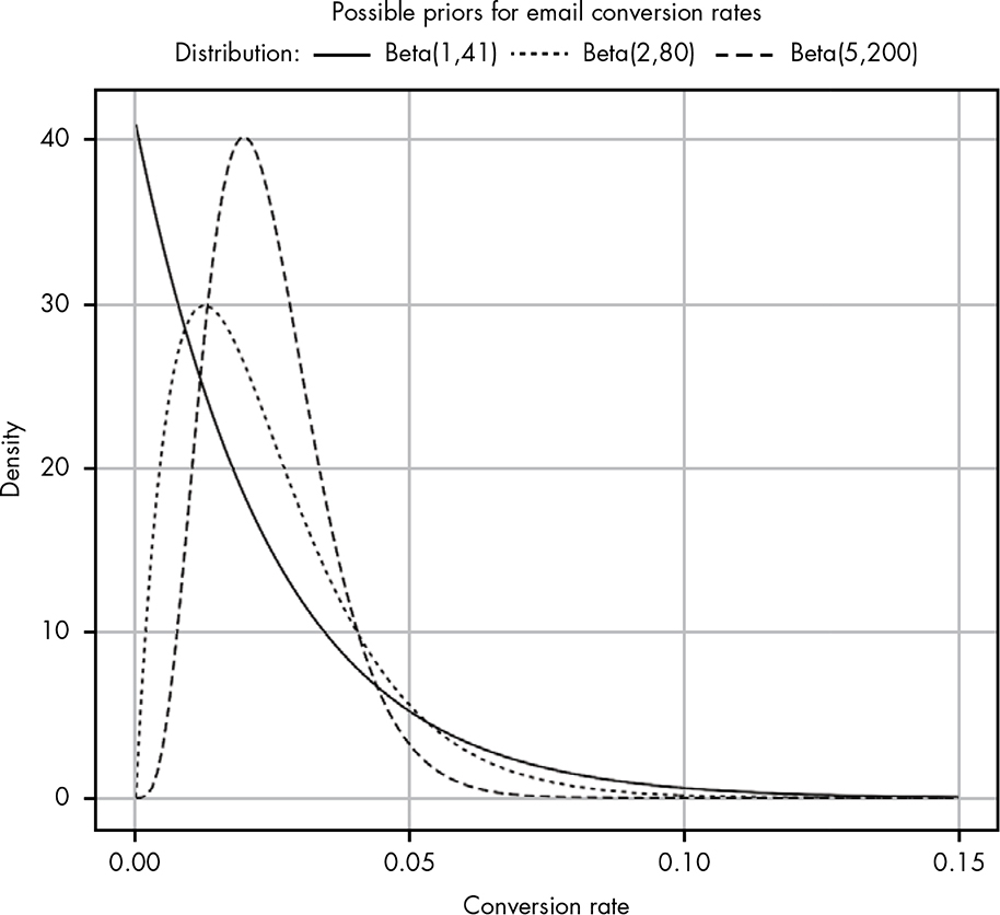
Figure 14-3: Comparing different possible prior probabilities
As you can see, the lower the combined α + β, the wider our distribution. The problem now is that even the most liberal option we have, Beta(1,41), seems a little too pessimistic, as it puts a lot of our probability density in very low values. We’ll stick with this distribution nonetheless, since it is based on the 2.4 percent conversion rate in the data from the email provider, and is the weakest of our priors. Being a “weak” prior means it will be more easily overridden by actual data as we collect more of it. A stronger prior, like Beta(5,200), would take more evidence to change (we’ll see how this happens next). Deciding whether or not to use a strong prior is a judgment call based on how well you expect the prior data to describe what you’re currently doing. As we’ll see, even a weak prior can help keep our estimates more realistic when we’re working with small amounts of data.
Remember that, when working with the beta distribution, we can calculate our posterior distribution (the combination of our likelihood and our prior) by simply adding together the parameters for the two beta distributions:
Beta(αposterior, βposterior) = Beta(αlikelihood + αprior, βlikelihood + βprior)
Using this formula, we can compare our beliefs with and without priors, as shown in Figure 14-4.
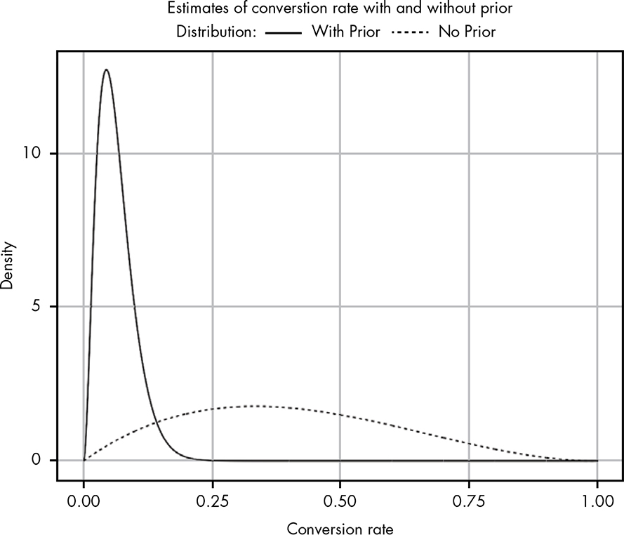
Figure 14-4: Comparing our likelihood (no prior) to our posterior (with prior)
Wow! That’s quite sobering. Even though we’re working with a relatively weak prior, we can see that it has made a huge impact on what we believe are realistic conversion rates. Notice that for the likelihood with no prior, we have some belief that our conversion rate could be as high as 80 percent. As mentioned, this is highly suspicious; any experienced email marketer would tell you than an 80 percent conversion rate is unheard of. Adding a prior to our likelihood adjusts our beliefs so that they become much more reasonable. But I still think our updated beliefs are a bit pessimistic. Maybe the email’s true conversion rate isn’t 40 percent, but it still might be better than this current posterior distribution suggests.
How can we prove that our blog has a better conversion rate than the sites in the email provider’s data, which have a 2.4 percent conversion rate? The way any rational person does: with more data! We wait a few hours to gather more results and now find that out of 100 people who opened your email, 25 have clicked the link! Let’s look at the difference between our new posterior and likelihood, shown in Figure 14-5.
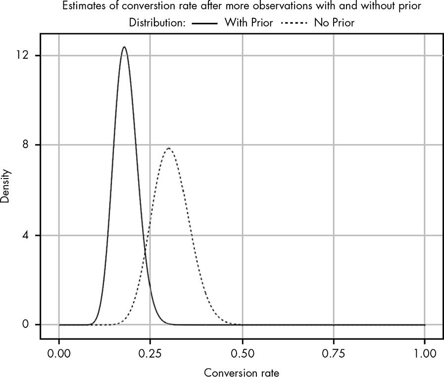
Figure 14-5: Updating our beliefs with more data
As we continue to collect data, we see that our posterior distribution using a prior is starting to shift toward the one without the prior. Our prior is still keeping our ego in check, giving us a more conservative estimate for the true conversion rate. However, as we add evidence to our likelihood, it starts to have a bigger impact on what our posterior beliefs look like. In other words, the additional observed data is doing what it should: slowly swaying our beliefs to align with what it suggests. So let’s wait overnight and come back with even more data!
In the morning we find that 300 subscribers have opened their email, and 86 of those have clicked through. Figure 14-6 shows our updated beliefs.
What we’re witnessing here is the most important point about Bayesian statistics: the more data we gather, the more our prior beliefs become diminished by evidence. When we had almost no evidence, our likelihood proposed some rates we know are absurd (e.g., 80 percent click-through), both intuitively and from personal experience. In light of little evidence, our prior beliefs squashed any data we had.
But as we continue to gather data that disagrees with our prior, our posterior beliefs shift toward what our own collected data tells us and away from our original prior.
Another important takeaway is that we started with a pretty weak prior. Even then, after just a day of collecting a relatively small set of information, we were able to find a posterior that seems much, much more reasonable.
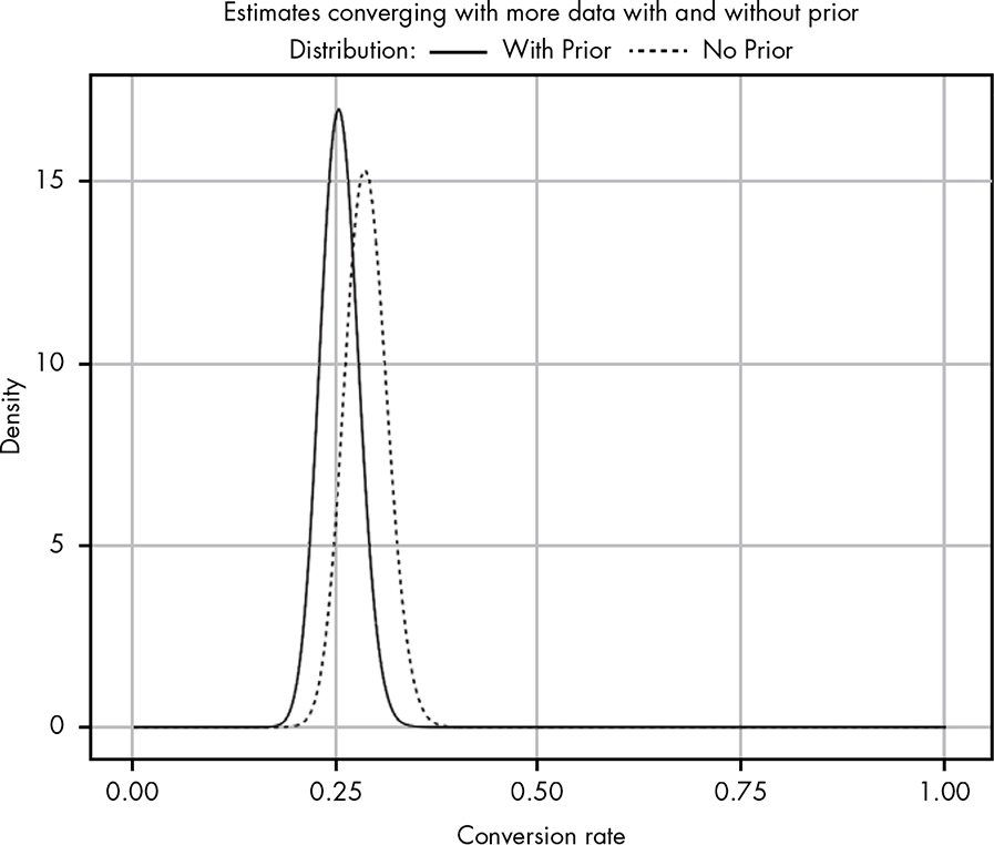
Figure 14-6: Our posterior beliefs with even more data added
The prior probability distribution in this case helped tremendously with keeping our estimate much more realistic in the absence of data. This prior probability distribution was based on real data, so we could be fairly confident that it would help us get our estimate closer to reality. However, in many cases we simply don’t have any data to back up our prior. So what do we do then?
Prior as a Means of Quantifying Experience
Because we knew the idea of an 80 percent click-through rate for emails was laughable, we used data from our email provider to come up with a better estimate for our prior. However, even if we didn’t have data to help establish our prior, we could still ask someone with a marketing background to help us make a good estimate. A marketer might know from personal experience that you should expect about a 20 percent conversion rate, for example.
Given this information from an experienced professional, you might choose a relatively weak prior like Beta(2,8) to suggest that the expected conversion rate should be around 20 percent. This distribution is just a guess, but the important thing is that we can quantify this assumption. For nearly every business, experts can often provide powerful prior information based simply on previous experience and observation, even if they have no training in probability specifically.
By quantifying this experience, we can get more accurate estimates and see how they can change from expert to expert. For example, if a marketer is certain that the true conversion rate should be 20 percent, we might model this belief as Beta(200,800). As we gather data, we can compare models and create multiple confidence intervals that quantitatively model any expert beliefs. Additionally, as we gain more and more information, the difference due to these prior beliefs will decrease.
Is There a Fair Prior to Use When We Know Nothing?
There are certain schools of statistics that teach that you should always add 1 to both α and β when estimating parameters with no other prior. This corresponds to using a very weak prior that holds that each outcome is equally likely: Beta(1,1). The argument is that this is the “fairest” (i.e., weakest) prior we can come up with in the absence of information. The technical term for a fair prior is a noninformative prior. Beta(1,1) is illustrated in Figure 14-7.
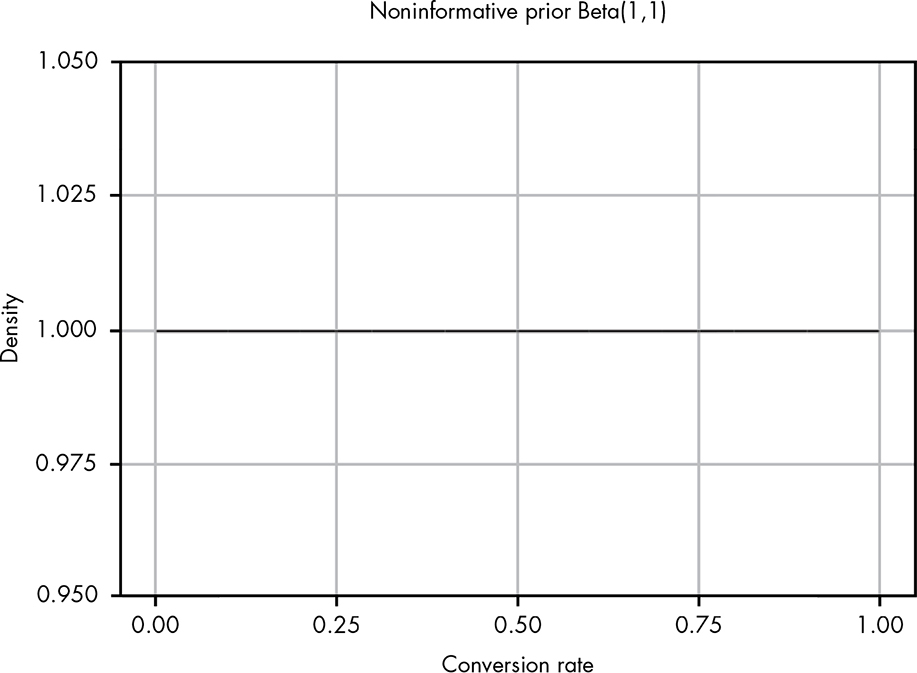
Figure 14-7: The noninformative prior Beta(1,1)
As you can see, this is a perfectly straight line, so that all outcomes are then equally likely and the mean likelihood is 0.5. The idea of using a noninformative prior is that we can add a prior to help smooth out our estimate, but that prior isn’t biased toward any particular outcome. However, while this may initially seem like the fairest way to approach the problem, even this very weak prior can lead to some strange results when we test it out.
Take, for example, the probability that the sun will rise tomorrow. Say you are 30 years old, and so you’ve experienced about 11,000 sunrises in your lifetime. Now suppose someone asks the probability that the sun will rise tomorrow. You want to be fair and use a noninformative prior, Beta(1,1). The distribution that represents your belief that the sun will not rise tomorrow would be Beta(1,11001), based on your experiences. While this gives a very low probability for the sun not rising tomorrow, it also suggests that we would expect to see the sun not rise at least once by the time you reach 60 years old. The so-called “noninformative” prior is providing a pretty strong opinion about how the world works!
You could argue that this is only a problem because we understand celestial mechanics, so we already have strong prior information we can’t forget. But the real problem is that we’ve never observed the case where the sun doesn’t rise. If we go back to our likelihood function without the noninformative prior, we get Beta(0,11000).
However, when either α or β ≤ 0, the beta distribution is undefined, which means that the correct answer to “What is the probability that the sun will rise tomorrow?” is that the question doesn’t make sense because we’ve never seen a counterexample.
As another example, suppose you found a portal that transported you and a friend to a new world. An alien creature appears before you and fires a strange-looking gun at you that just misses. Your friend asks you, “What’s the probability that the gun will misfire?” This is a completely alien world and the gun looks strange and organic, so you know nothing about its mechanics at all.
This is, in theory, the ideal scenario for using a noninformative prior, since you have absolutely no prior information about this world. If you add your noninformative prior, you get a posterior Beta(1,2) probability that the gun will misfire (we observed α = 0 misfires and β = 1 successful fires). This distribution tells us the mean posterior probability of a misfire is 1/3, which seems astoundingly high given that you don’t even know if the strange gun can misfire. Again, even though Beta(0,1) is undefined, using it seems like the rational approach to this problem. In the absence of sufficient data and any prior information, your only honest option is to throw your hands in the air and tell your friend, “I have no clue how to even reason about that question!”
The best priors are backed by data, and there is never really a true “fair” prior when you have a total lack of data. Everyone brings to a problem their own experiences and perspective on the world. The value of Bayesian reasoning, even when you are subjectively assigning priors, is that you are quantifying your subjective belief. As we’ll see later in the book, this means you can compare your prior to other people’s and see how well it explains the world around you. A Beta(1,1) prior is sometimes used in practice, but you should use it only when you earnestly believe that the two possible outcomes are, as far as you know, equally likely. Likewise, no amount of mathematics can make up for absolute ignorance. If you have no data and no prior understanding of a problem, the only honest answer is to say that you can’t conclude anything at all until you know more.
All that said, it’s worth noting that this topic of whether to use Beta(1,1) or Beta(0,0) has a long history, with many great minds arguing various positions. Thomas Bayes (namesake of Bayes’ theorem) hesitantly believed in Beta(1,1); the great mathematician Simon-Pierre Laplace was quite certain Beta(1,1) was correct; and the famous economist John Maynard Keynes thought using Beta(1,1) was so preposterous that it discredited all of Bayesian statistics!
Wrapping Up
In this chapter, you learned how to incorporate prior information about a problem to arrive at much more accurate estimates for unknown parameters. When we have only a little information about a problem, we can easily get probabilistic estimates that seem impossible. But we might have prior information that can help us make better inferences from that small amount of data. By adding this information to our estimates, we get much more realistic results.
Whenever possible, it’s best to use a prior probability distribution based on actual data. However, often we won’t have data to support our problem, but we either have personal experience or can turn to experts who do. In these cases, it’s perfectly fine to estimate a probability distribution that corresponds to your intuition. Even if you’re wrong, you’ll be wrong in a way that is recorded quantitatively. Most important, even if your prior is wrong, it will eventually be overruled by data as you collect more observations.
Exercises
Try answering the following questions to see how well you understand priors. The solutions can be found in Appendix C.
- Suppose you’re playing air hockey with some friends and flip a coin to see who starts with the puck. After playing 12 times, you realize that the friend who brings the coin almost always seems to go first: 9 out of 12 times. Some of your other friends start to get suspicious. Define prior probability distributions for the following beliefs:
- One person who weakly believes that the friend is cheating and the true rate of coming up heads is closer to 70 percent.
- One person who very strongly trusts that the coin is fair and provided a 50 percent chance of coming up heads.
- One person who strongly believes the coin is biased to come up heads 70 percent of the time.
- To test the coin, you flip it 20 more times and get 9 heads and 11 tails. Using the priors you calculated in the previous question, what are the updated posterior beliefs in the true rate of flipping a heads in terms of the 95 percent confidence interval?