B
ENOUGH CALCULUS TO GET BY

In this book, we’ll occasionally use ideas from calculus, though no actual manual solving of calculus problems will be required! What will be required is an understanding of some of the basics of calculus, such as the derivative and (especially) the integral. This appendix is by no means an attempt to teach these concepts deeply or show you how to solve them; instead, it offers a brief overview of these ideas and how they’re represented in mathematical notation.

Functions

A function is just a mathematical “machine” that takes one value, does something with it, and returns another value. This is very similar to how functions in R work (see Appendix A): they take in a value and return a result. For example, in calculus we might have a function called f defined like this:

f(x) = x²

In this example, f takes a value, x, and squares it. If we input the value 3 into f, for example, we get:

f(3) = 9

This is a little different than how you might have seen it in high school algebra, where you’d usually have a value y and some equation involving x.

y = x²

One reason why functions are important is that they allow us to abstract away the actual calculations we’re doing. That means we can say something like y = f(x), and just concern ourselves with the abstract behavior of the function itself, not necessarily how it’s defined. That’s the approach we’ll take for this appendix.

As an example, say you’re training to run a 5 km race and you’re using a smartwatch to keep track of your distance, speed, time, and other factors. You went out for a run today and ran for half an hour. However, your smartwatch malfunctioned and recorded only your speed in miles per hour (mph) throughout your 30-minute run. Figure B-1 shows the data you were able to recover.

For this appendix, think of your running speed as being created by a function, s, that takes an argument t, the time in hours. A function is typically written in terms of the argument it takes, so we would write s(t), which results in a value that gives your current speed at time t. You can think of the function s as a machine that takes the current time and returns your speed at that time. In calculus, we’d usually have a specific definition of s(t), such as s(t) = t² + 3t + 2, but here we’re just talking about general concepts, so we won’t worry about the exact definition of s.

From this function alone, we can learn a few things. It’s clear that your pace was a little uneven during this run, going up and down from a high of nearly 8 mph near the end and a low of just under 4.5 mph in the beginning.

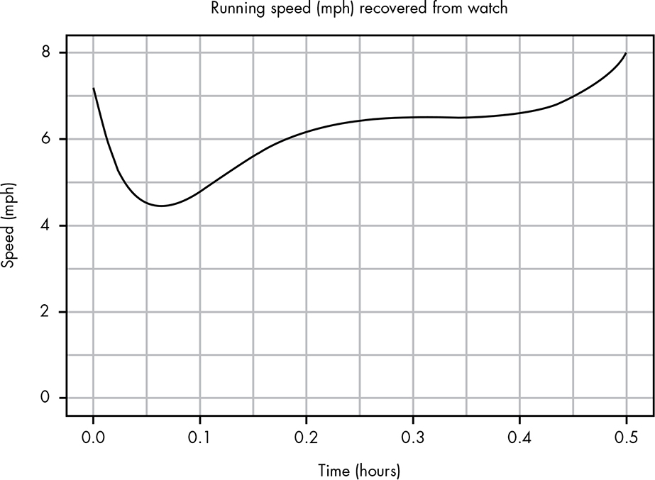
Figure B-1: The speed for a given time in your run

However, there are still a lot of interesting questions you might want to answer, such as:

• How far did you run?
• When did you lose the most speed?
• When did you gain the most speed?
• During what times was your speed relatively consistent?

We can make a fairly accurate estimate of the last question from this plot, but the others seem impossible to answer from what we have. However, it turns out that we can answer all of these questions with the power of calculus! Let’s see how.

Determining How Far You’ve Run

So far our chart just shows your running speed at a certain time, so how do we find out how far you’ve run?

This doesn’t sound too difficult in theory. Suppose, for example, you ran 5 mph consistently for the whole run. In that case, you ran 5 mph for 0.5 hour, so your total distance was 2.5 miles. This intuitively makes sense, since you would have run 5 miles each hour, but you ran for only half an hour, so you ran half the distance you would have run in an hour.

But our problem involves a different speed at nearly every moment that you were running. Let’s look at the problem another way. Figure B-2 shows the plotted data for a constant running speed.

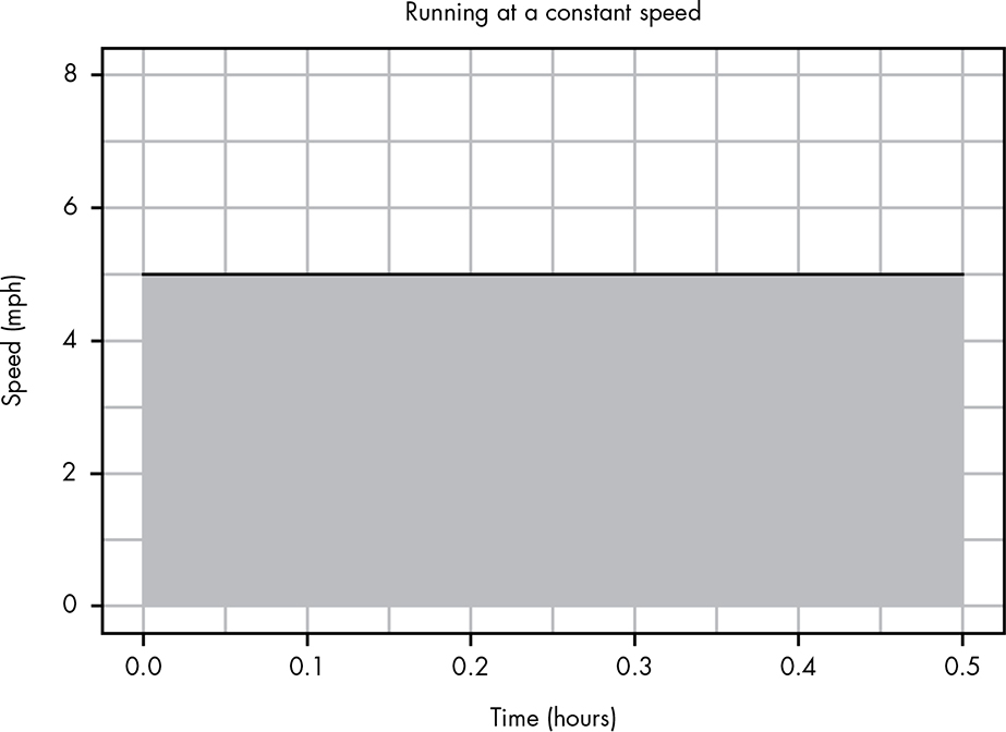
Figure B-2: Visualizing distance as the area of the speed/time plot

You can see that this data creates a straight line. If we think about the space under this line, we can see that it’s a big block that actually represents the distance you’ve run! The block is 5 high and 0.5 long, so the area of this block is 5 × 0.5 = 2.5, which gives us the 2.5 miles result!

Now let’s look at a simplified problem with varying speeds, where you ran 4.5 mph from 0.0 to 0.3 hours, 6 mph from 0.3 to 0.4 hours, and 3 mph the rest of the way to 0.5 miles. If we visualize these results as blocks, or towers, as in Figure B-3, we can solve our problem the same way.

The first tower is 4.5 × 0.3, the second is 6 × 0.1, and the third is 3 × 0.1, so that:

4.5 × 0.3 + 6 × 0.1 + 3 × 0.1 = 2.25

By looking at the area under the tower, then, we get the total distance you traveled: 2.25 miles.

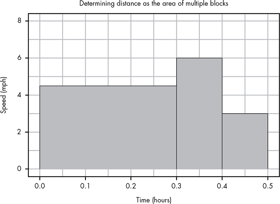
Figure B-3: We can easily calculate your total distance traveled by adding together these towers.

Measuring the Area Under the Curve: The Integral

You’ve now seen that we can figure out the area under the line to tell us how far you traveled. Unfortunately, the line for our original data is curved, which makes our problem a bit difficult: how can we calculate the towers under our curvy line?

We can start this process by imagining some large towers that are fairly close to the pattern of our curve. If we start with just three towers, as we can see in Figure B-4, it isn’t a bad estimate.

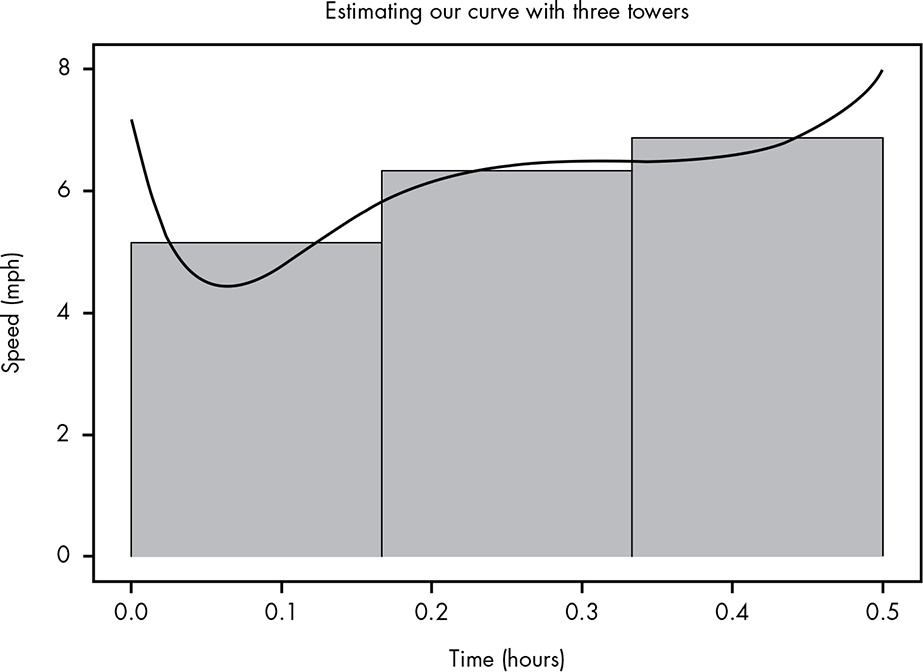
Figure B-4: Approximating the curve with three towers

By calculating the area under each of these towers, we get a value of 3.055 miles for your estimated total miles traveled. But we could clearly do better by making more, smaller towers, as shown in Figure B-5.

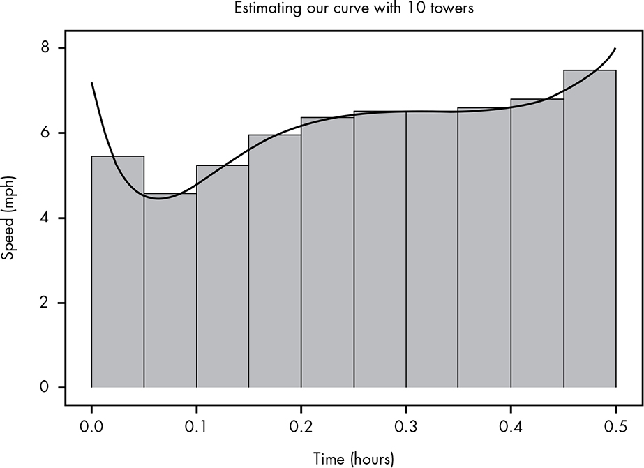
Figure B-5: Approximating the curve better by using 10 towers instead of 3

Adding up the areas of these towers, we get 3.054 miles, which is a more accurate estimate.

If we imagine repeating this process forever, using more and thinner towers, eventually we would get the full area under the curve, as in Figure B-6.

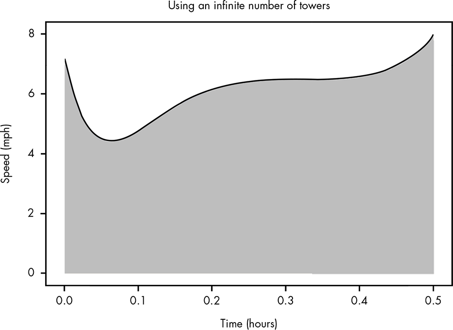
Figure B-6: Completely capturing the area under the curve

This represents the exact area traveled for your half-hour run. If we could add up infinitely many towers, we would get a total of 3.053 miles. Our estimates were pretty close, and as we use more and smaller towers, our estimate gets closer. The power of calculus is that it allows us to calculate this exact area under the curve, or the integral. In calculus, we’d represent the integral for our s(t) from 0 to 0.5 in mathematical notation as:

That ∫ is just a fancy S, meaning the sum (or total) of the area of all the little towers in s(t). The dt notation reminds us that we’re talking about little bits of the variable t; the d is a mathematical way to refer to these little towers. Of course, in this bit of notation, there’s only one variable, t, so we aren’t likely to get confused. Likewise, in this book, we typically drop the dt (or its equivalent for the variable being used) since it’s obvious in the examples.

In our last notation we set the beginning and end of our integral, which means we can find the distance not just for the whole run but also for a section of it. Suppose we wanted to know how far you ran between 0.1 to 0.2 of an hour. We would note this as:

We can visualize this integral as shown in Figure B-7.

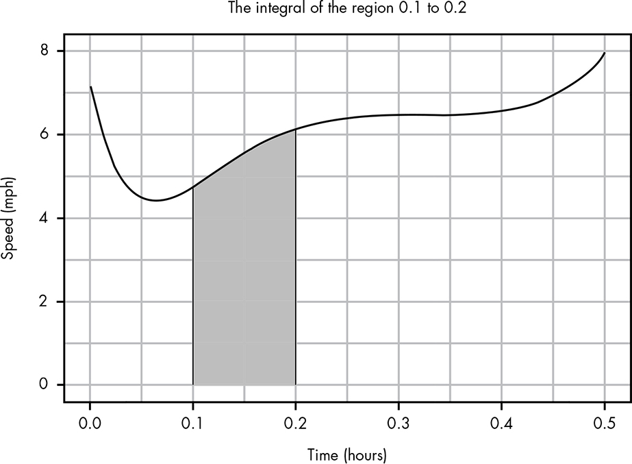
Figure B-7: Visualizing the area under the curve for the region from 0.1 to 0.2

The area of just this shaded region is 0.556 miles.

We can even think of the integral of our function as another function. Suppose we define a new function, dist(T), where T is our “total time run”:

This gives us a function that tells us the distance you’ve traveled at time T. We can also see why we want to use dt because we can see that our integral is being applied to the lowercase t argument rather than the capital T argument. Figure B-8 plots this out to the total distance you’ve run at any given time T during your run.

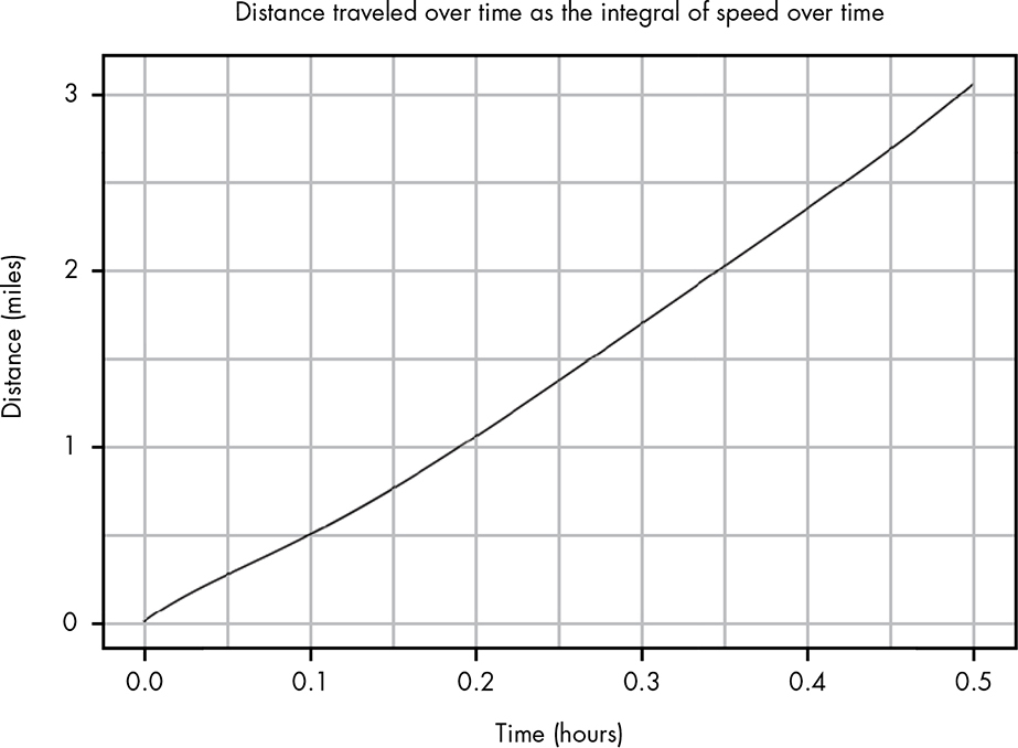
Figure B-8: Plotting out the integral transforms a time and speed plot to a time and distance plot.

In this way, the integral has transformed our function s, which was “speed at a time,” to a function dist, “distance covered at a time.” As shown earlier, the integral of our function between two points represents the distance traveled between two different times. Now we’re looking at the total distance traveled at any given time t from the beginning time of 0.

The integral is important because it allows us to calculate the area under curves, which is much trickier to calculate than if we have straight lines. In this book, we’ll use the concept of the integral to determine the probabilities that events are between two ranges of values.

Measuring the Rate of Change: The Derivative

You’ve seen how we can use the integral to figure out the distance traveled when all we have is a recording of your speed at various times. But with our varying speed measurements, we might also be interested in figuring out the rate of change for your speed at various times. When we talk about the rate at which speed is changing, we’re referring to acceleration. In our chart, there are a few interesting points regarding the rate of change: the points when you’re losing speed the fastest, when you’re gaining speed the fastest, and when the speed is the most steady (i.e., the rate of change is near 0).

Just as with integration, the main challenge of figuring out your acceleration is that it seems to always be changing. If we had a constant rate of change, calculating the acceleration isn’t that difficult, as shown in Figure B-9.

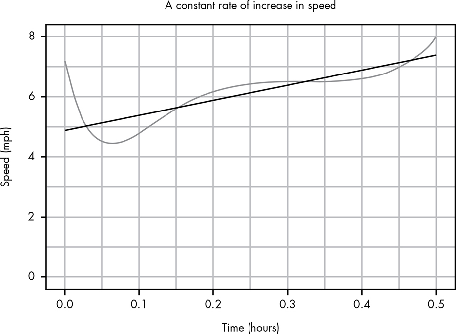
Figure B-9: Visualizing a constant rate of change (compared with your actual changing rate)

You might remember from basic algebra that we can draw any line using this formula:

y = mx + b

where b is the point at which the line crosses the y-axis and m is the slope of the line. The slope represents the rate of change of a straight line. For the line in Figure B-9, the full formula is:

y = 5x + 4.8

The slope of 5 means that for every time x grows by 1, y grows by 5; 4.8 is the point at which the line crosses the x-axis. In this example, we’d interpret this formula as s(t) = 5t + 4.8, meaning that for every mile you travel you accelerate by 5 mph, and that you started off at 4.8 mph. Since you’ve run half a mile, using this simple formula, we can figure out:

s(t) = 5 × 0.5 + 4.8 = 7.3

which means at the end of your run, you would be traveling 7.3 mph. We could similarly determine your exact speed at any point in the run, as long as the acceleration is constant!

For our actual data, because the line is curvy it’s not easy to determine the slope at a single point in time. Instead, we can figure out the slopes of parts of the line. If we divide our data into three subsections, we could draw lines between each part as in Figure B-10.

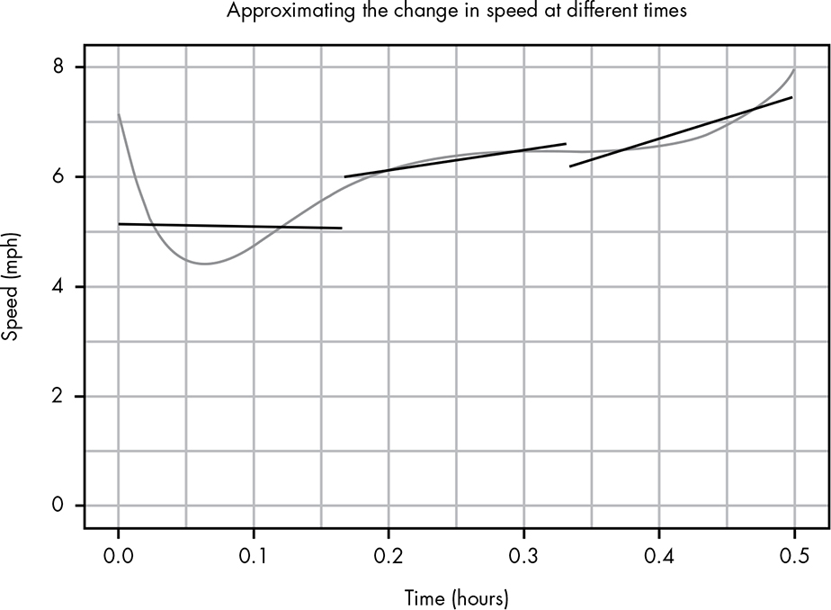
Figure B-10: Using multiple slopes to get a better estimate of your rate of change

Now, clearly these lines aren’t a perfect fit to our curvy line, but they allow us to see the parts where you accelerated the fastest, slowed down the most, and were relatively stable.

If we split our function up into even more pieces we can get even better estimates, as in Figure B-11.

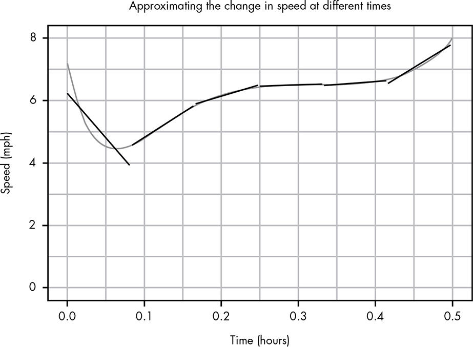
Figure B-11: Adding more slopes allows us to better approximate your curve.

Here we have a similar pattern to when we found the integral, where we split the area under the curve into smaller and smaller towers until we were adding up infinitely many small towers. Now we want to break up our line into infinitely many small line segments. Eventually, rather than a single m representing our slope, we have a new function representing the rate of change at each point in our original function. This is called the derivative, represented in mathematical notation like this:

Again, the dx just reminds us that we’re looking at very small pieces of our argument x. Figure B-12 shows the plot of the derivative for our s(t) function, which allows us to see the exact rate of speed change at each moment in your run. In other words, this is a plot of your acceleration during your run. Looking at the y-axis, you can see that you rapidly lost speed in the beginning, and at around 0.3 hours you had a period of 0 acceleration, meaning your pace did not change (this is usually a good thing when practicing for a race!). We can also see exactly when you gained the most speed. Looking at the original plot, we couldn’t easily tell if you were gaining speed faster around 0.1 hours (just after your first speedup) or at the end of your run. With the derivative, though, it’s clear that the final burst of speed at the end was indeed faster than at the beginning.

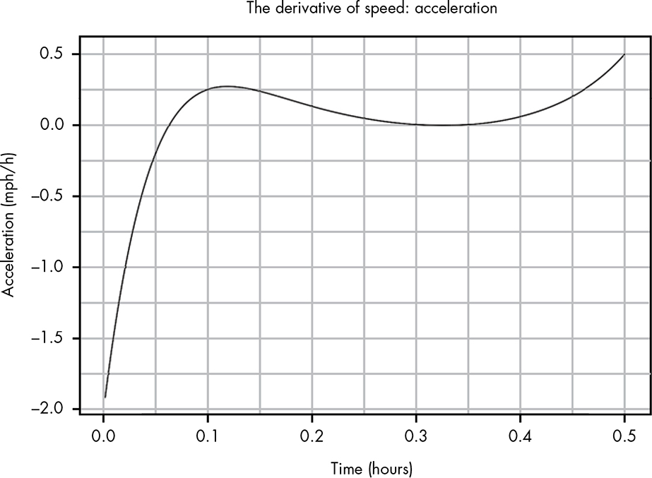
Figure B-12: The derivative is another function that describes the slope of s(x) at each point.

The derivative works just like the slope of a straight line, only it tells us how much a curvy line is sloping at a certain point.

The Fundamental Theorem of Calculus

We’ll look at one last truly remarkable calculus concept. There’s a very interesting relationship between the integral and the derivative. (Proving this relationship is far beyond the scope of this book, so we’ll focus only on the relationship itself here.) Suppose we have a function F(x), with a capital F. What makes this function special is that its derivative is f(x). For example, the derivative of our dist function is our s function; that is, your change in distance at each point in time is your speed. The derivative of speed is acceleration. We can describe this mathematically as:

In calculus terms we call F the antiderivative of f, because f is F’s derivative. Given our examples, the antiderivative of acceleration would be speed, and the antiderivative of speed would be distance. Now suppose for any value of f, we want to take its integral between 10 and 50; that is, we want:

We can get this simply by subtracting F(10) from F(50), so that:

The relationship between the integral and the derivative is called the fundamental theorem of calculus. It’s a pretty amazing tool, because it allows us to solve integrals mathematically, which is often much more difficult than finding derivatives. Using the fundamental theorem, if we can find the antiderivative of the function we want to find the integral of, we can easily perform integration. Figuring this out is the heart of performing integration by hand.

A full course on calculus (or two) typically explores the topics of integrals and derivatives in much greater depth. However, as mentioned, in this book we’ll only be making occasional use of calculus, and we’ll be using R for all of the calculations. Still, it’s helpful to have a rough understanding of what calculus and those unfamiliar ∫ symbols are all about!