CHAPTER 7

LOGICAL DATABASE DESIGN

Logical database design is the process of deciding how to arrange the attributes of the entities in a given business environment into database structures, such as the tables of a relational database. The goal of logical database design is to create well structured tables that properly reflect the company's business environment. The tables will be able to store data about the company's entities in a non-redundant manner and foreign keys will be placed in the tables so that all the relationships among the entities will be supported. Physical database design, which will be treated in the next chapter, is the process of modifying the logical database design to improve performance.

OBJECTIVES

• Describe the concept of logical database design.
• Design relational databases by converting entity-relationship diagrams into relational tables.
• Describe the data normalization process.
• Perform the data normalization process.
• Test tables for irregularities using the data normalization process.
• Learn basic SQL commands to build data structures.
• Learn basic SQL commands to manipulate data.

CHAPTER OUTLINE

• Introduction
• Converting E-R Diagrams into Relational Tables
  • Introduction
  • Converting a Simple Entity
  • Converting Entities in Binary Relationships
  • Converting Entities in Unary Relationships
  • Converting Entities in Ternary Relationships
  • Designing the General Hardware Co. Database
  • Designing the Good Reading Bookstores Database
  • Designing the World Music Association Database
  • Designing the Lucky Rent-A-Car Database
• The Data Normalization Process
  • Introduction to the Data Normalization Technique
  • Steps in the Data Normalization Process
  • Example: General Hardware Co.
  • Example: Good Reading Bookstores
  • Example: World Music Association
  • Example: Lucky Rent-A-Car
• Testing Tables Converted from E-R
  • Diagrams
  • with Data Normalization
• Building the Data Structure with SQL
• Manipulating the Data with SQL
• Summary

INTRODUCTION

Historically, a number of techniques have been used for logical database design. In the 1970s, when the hierarchical and network approaches to database management were the only ones available, a technique known as data normalization was developed. While data normalization has some very useful features, it was difficult to apply in that environment. Data normalization can also be used to design relational databases and, actually, is a better fit for relational databases than it was for the hierarchical and network databases. But, as the relational approach to database management and the entity-relationship approach to data modeling both blossomed in the 1980s, a very natural and pleasing approach to logical database design evolved in which rules were developed to convert E-R diagrams into relational tables. Optionally, the result of this process can then be tested with the data normalization technique. Thus, this chapter on the logical design of relational databases will proceed in three parts: first, the conversion of E-R diagrams into relational tables, then the data normalization technique, and finally the use of the data normalization technique to test the tables resulting from the E-R diagram conversions.

CONVERTING E-R DIAGRAMS INTO RELATIONAL TABLES

Introduction

Converting entity-relationship diagrams to relational tables is surprisingly straightforward, with just a few simple rules to follow. Basically, each entity will convert to a table, plus each many-to-many relationship or associative entity will convert to a table. The only other issue is that during the conversion, certain rules must be followed to ensure that foreign keys appear in their proper places in the tables. We will demonstrate these techniques by methodically converting the E-R diagrams of Chapter 2 into relational tables.

Converting a Simple Entity

Figure 7.1 repeats the simple entity box in Figure 2.1. Figure 7.2 shows a relational table that can store the data represented in the entity box. The table simply contains the attributes that were specified in the entity box. Notice that Salesperson Number is underlined to indicate that it is the unique identifier of the entity, and the primary key of the table. Clearly, the more interesting issues and rules come about when, as almost always happens, entities are involved in relationships with other entities.

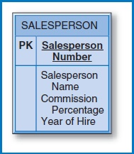
FIGURE 7.1 The entity box from Figure 2.1

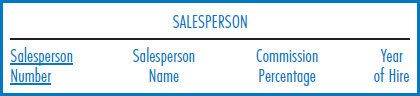
FIGURE 7.2 Conversion of an E-R diagram entity box to a relational table

Converting Entities in Binary Relationships

One-to-One Binary Relationship Figure 7.3 repeats the one-to-one binary relationship of Figure 2.4a. There are three options for designing tables to represent this data, as shown in Figure 7.4. In Figure 7.4a, the two entities are combined into one relational table. On the one hand, this is possible because the one-to-one relationship means that for one salesperson, there can only be one associated office and conversely, for one office there can be only one salesperson. So a particular salesperson and office combination can fit together in one record, as shown in Figure 7.4a. On the other hand, this design is not a good choice for two reasons. One reason is that the very fact that salesperson and office were drawn in two different entity boxes in the E-R diagram of Figure 7.3 means that they are thought of separately in this business environment and thus should be kept separate in the database. The other reason is the modality of zero at the salesperson in Figure 7.3. Reading that diagram from right to left, it says that an office might have no one assigned to it. Thus, in the table in Figure 7.4a, there could be a few or possibly many record occurrences that have values for the office number, telephone, and size attributes but have the four attributes pertaining to salespersons empty or null! This could result in a lot of wasted storage space, but it is worse than that. If Salesperson Number is declared to be the primary key of the table, this scenario would mean that there would be records with no primary key values, a situation which is clearly not allowed.

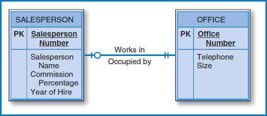
FIGURE 7.3 The one-to-one (1-1) binary relationship from Figure 2.4a

Figure 7.4b is a better choice. There are separate tables for the salesperson and office entities. In order to record the relationship, i.e. which salesperson is assigned to which office, the Office Number attribute is placed as a foreign key in the SALESPERSON table. This connects the salespersons with the offices to which they are assigned. Again, look at the modalities in the E-R diagram in Figure 7.3. Reading from left to right, each salesperson is assigned to exactly one office (indicated by the two “ones” adjacent to the office entity). That translates directly into each record in the SALESPERSON table of Figure 7.4b having a value (and a single value, at that) for its Office Number foreign key attribute. That's good! But what about the problem of unassigned offices mentioned in the previous paragraph? In Figure 7.4b, unassigned offices will each have a record in the OFFICE table, with Office Number as the primary key, which is fine. Their office numbers will simply not appear as foreign key values in the SALESPERSON table.

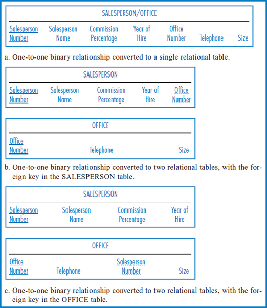
FIGURE 7.4 Conversion of an E-R diagram with two entities in a one-to-one binary relationship into one or two relational tables

Finally, instead of placing Office Number as a foreign key in the SALESPERSON table, could you instead place Salesperson Number as a foreign key in the OFFICE table, Figure 7.4c? Recall that, reading the E-R diagram of Figure 7.3 from right to left, the modality of zero adjacent to the salesperson entity says that an office might be empty, i.e. it might not be assigned to any salesperson. But then, some or perhaps many records of the OFFICE table of Figure 7.4c would have no value or a null in their Salesperson Number foreign key attribute positions. Why bother having to deal with this situation when the design in Figure 7.4b avoids it?

Certainly, it follows that if the modalities were reversed, meaning that the zero modality was adjacent to the office entity box and the one modality was adjacent to the salesperson entity box, then the design in Figure 7.4c would be the preferable one. This would mean that every office must have a salesperson assigned to it but a salesperson may or may not be assigned to an office. Perhaps lots of the salespersons travel most of the time and don't need offices. By the way, while we're in “what if” mode, what if the modality was zero on both sides? Then there would be a judgment call to make between the designs of Figure 7.4b and Figure 7.4c. If the goal is to minimize the number of null values in the foreign key, then you have to decide whether it is more likely that a salesperson is not assigned to an office (Figure 7.4c is preferable) or that an office is empty (Figure 7.4b is preferable).

One-to-Many Binary Relationship Figure 7.5 (copied from Figure 2.4b) shows an E-R diagram for a one-to-many binary relationship. Figure 7.6 shows the conversion of this E-R diagram into two relational tables. This is, perhaps, the simplest case of all. The rule is that the unique identifier of the entity on the “one side” of the one-to-many relationship is placed as a foreign key in the table representing the entity on the “many side.” In this case, the Salesperson Number attribute is placed in the CUSTOMER table as a foreign key. Each salesperson has one record in the SALESPERSON table, as does each customer in the CUSTOMER table. The Salesperson Number attribute in the CUSTOMER table links the two and, since the E-R diagram tells us that every customer must have a salesperson, there are no empty attributes in the CUSTOMER table records.

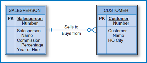
FIGURE 7.5 The one-to-many (1-M) binary relationship from Figure 2.4b

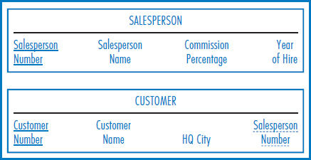
FIGURE 7.6 Conversion of an E-R diagram with two entities in a one-to-many binary relationship into two relational tables

Many-to-Many Binary Relationship Figure 7.7 shows the E-R diagram with the many-to-many binary relationship from Figure 2.5. The equivalent diagram from Figure 2.6, using an associative entity, is shown in Figure 7.8. An E-R diagram with two entities in a many-to-many relationship converts to three relational tables, as shown in Figure 7.9. Each of the two entities converts to a table with its own attributes but with no foreign keys (regarding this relationship). The SALESPERSON table and the PRODUCT table in Figure 7.9 each contain only the attributes shown in the salesperson and product entity boxes of Figure 7.7 and Figure 7.8.

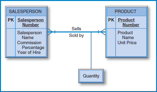
FIGURE 7.7 The many-to-many binary relationship from Figure 2.5

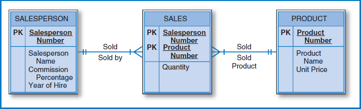
FIGURE 7.8 The associative entity from Figure 2.6

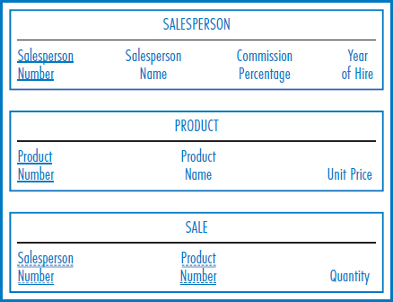
FIGURE 7.9 Conversion of an E-R diagram in Figure 7.7 (and Figure 7.8) with two entities in a many-to-many binary relationship into three relational tables

In addition, there must be a third “many-to-many” table for the many-to-many relationship, the reasons for which were explained in Chapter 5. The primary key of this additional table is the combination of the unique identifiers of the two entities in the many-to-many relationship. Additional attributes consist of the intersection data, Quantity in this example. Also as explained in Chapter 5, there are circumstances in which additional attributes, such as date and timestamp attributes, must be added to the primary key of the many-to-many table to achieve uniqueness.

Converting Entities in Unary Relationships

One-to-One Unary Relationship Figure 7.10 repeats the E-R diagram with a one-to-one unary relationship from Figure 2.7a. In this case, with only one entity type involved and with a one-to-one relationship, the conversion requires only one table, as shown in Figure 7.11. For a particular salesperson, the Backup Number attribute represents the salesperson number of his backup person, i.e. the person who handles his accounts when he is away for any reason.

FIGURE 7.10 The one-to-one (1-1) unary relationship from Figure 2.7a

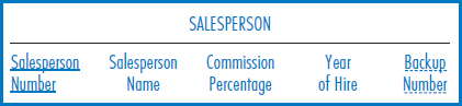
FIGURE 7.11 Conversion of the E-R diagram in Figure 7.10 with a one-to-one unary relationship into a relational table

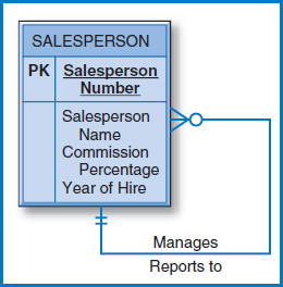
FIGURE 7.12 The one-to-many (1-M) unary relationship from Figure 2.7b

One-to-Many Unary Relationship The one-to-many unary relationship situation is very similar to the one-to-one unary case. Figure 7.12 repeats the E-R diagram from Figure 2.7b. Figure 7.13 shows the conversion of this diagram into a relational database. Some employees manage other employees. An employee's manager is recorded in the Manager Number attribute in the table in Figure 7.13. The manager numbers are actually salesperson numbers since some salespersons are sales managers who manage other salespersons. This arrangement works because each employee has only one manager. For any particular SALESPERSON record, there can only be one value for the Manager Number attribute. However, if you scan down the Manager Number column, you will see that a particular value may appear several times because a person can manage several other salespersons.

Many-to-Many Unary Relationship Figure 7.14 shows the E-R diagram for the many-to-many unary relationship of Figure 2.7c. As Figure 7.15 indicates, this relationship requires two tables in the conversion. The PRODUCT table has no foreign keys. The COMPONENT table indicates which items go into making up which other items, as was described in the bill-of-materials discussion in Chapter 6. This table also contains any intersection data that may exist in the many-to-many relationship. In this example, the Quantity attribute indicates how many of a particular item go into making up another item.

The fact that we wind up with two tables in this conversion is really not surprising. The general rule is that in the conversion of a many-to-many relationship of any degree (unary, binary, or ternary), the number of tables will be equal to the number of entity types (one, two, or three, respectively) plus one more table for the many-to-many relationship. Thus, the conversion of the many-to-many unary relationship required two tables, the many-to-many binary relationship three tables, and, as will be shown next, the many-to-many ternary relationship four tables.

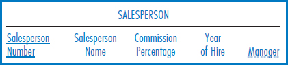
FIGURE 7.13 Conversion of the E-R diagram in Figure 7.12 with a one-to-many unary relationship into a relational table

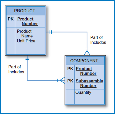
FIGURE 7.14 The many-to-many unary relationship from Figure 2.7c

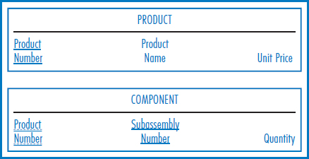
FIGURE 7.15 Conversion of the E-R diagram in Figure 7.14 with a many-to-many unary relationship into two relational tables

Converting Entities in Ternary Relationships

Finally, Figure 7.16 repeats the E-R diagram with the ternary relationship from Figure 2.8. Figure 7.17 shows the four tables necessary for the conversion to relational tables. Notice that the primary key of the SALE table, which is the table added for the many-to-many relationship, is the combination of the unique identifiers of the three entities involved, plus the Date attribute. In this case, with the premise being that a particular salesperson can have sold a particular product to a particular customer on different days, the Date attribute is needed in the primary key to achieve uniqueness.

Designing the General Hardware Co. Database

Having explored the specific E-R diagram-to-relational database conversion rules, let's look at a few examples, beginning with the General Hardware Co. Figure 7.18 is the General Hardware E-R diagram. It is convenient to begin the database design process with an important, central E-R diagram entity, such as salesperson, that has relationships with several other entities. Thus, the relational database in Figure 7.19 includes a SALESPERSON table with the four salesperson attributes shown in Figure 7.18's salesperson entity box (plus the Office Number attribute, to which we will return shortly). To the right of the salesperson entity box in the E-R diagram, there is a one-to-many relationship (“Sells To”) between salespersons and customers. The database then includes a CUSTOMER table with the Salesperson Number attribute as a foreign key, because salesperson is on the “one side” of the one-to-many relationship and customer is on the “many side” of the one-to-many relationship.

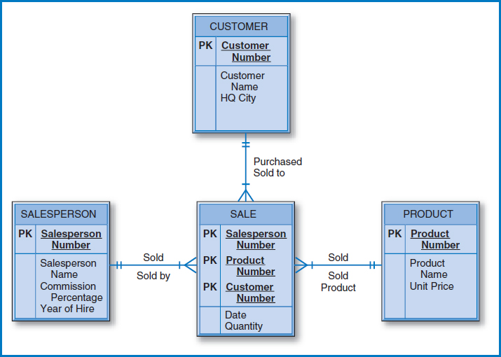
FIGURE 7.16 The ternary relationship from Figure 2.8

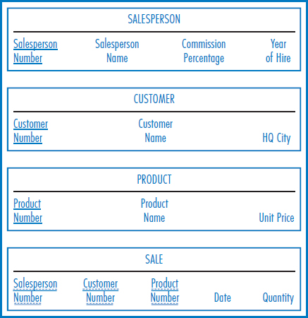
FIGURE 7.17 Conversion of the E-R diagram in Figure 7.16 with three entities in a ternary relationship into four relational tables

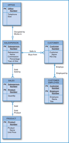
FIGURE 7.18 The General Hardware Company E-R diagram

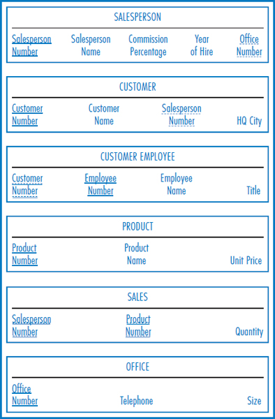
FIGURE 7.19 The General Hardware Company relational database

Customer employee is a dependent entity of customer and there is a one-to-many relationship between them. Because of this relationship, the CUSTOMER EMPLOYEE table in the database includes the Customer Number attribute as a foreign key. Furthermore, the Customer Number attribute is part of the primary key of the CUSTOMER EMPLOYEE table because customer employee is a dependent entity and we're told that employee numbers are unique only within a customer.

The PRODUCT table contains the three attributes of the product entity. The many-to-many relationship between the salesperson and product entities is represented by the SALES table in the database. Notice that the combination of the unique identifiers (Salesperson Number and Product Number) of the two entities in the many-to-many relationship is the primary key of the SALES table. Finally, the office entity has its table in the database with its three attributes, which brings us to the presence of the Office Number attribute as a foreign key in the SALESPERSON table. This is needed to maintain the one-to-one binary relationship between salesperson and office. A fair question is, since the relationship is “one” on both sides, why did we decide to put the foreign key in the SALESPERSON table rather than in the OFFICE table? The answer lies in the fact that the modality adjacent to SALESPERSON is zero while the modality adjacent to OFFICE is one. An office may or may not have a salesperson assigned to it but a salesperson must be assigned to an office. The result is that every salesperson must have an associated office number; the Office Number attribute in the SALESPERSON table can't be null. If we reversed it and put the Salesperson Number attribute in the OFFICE table, many of the Salesperson Number attribute values could be null since the zero modality going from office to salesperson tells us that an office can be empty.

One last thought: Why did the PRODUCT table end-up without any foreign keys? Because it is not the “target” (it is not on the “many side”) of any one-to-many binary relationship. It is also not involved in a one-to-one binary relationship that would require the presence of a foreign key. Finally, it is not involved in a unary relationship that would require repeating the primary key in the table.

Designing the Good Reading Bookstores Database

The Good Reading Bookstores' E-R diagram is repeated in Figure 7.20. Beginning with the central book entity and looking to its left, we see that there is a one-to-many relationship between books and publishers. A publisher publishes many books but a book is published by just one publisher. The Good Reading Bookstores relational database of Figure 7.2l shows the BOOK and PUBLISHER tables. Publisher Name is a foreign key in the BOOK table because publisher is on the “one side” of the one-to-many relationship and book is on the “many side.” Next is the AUTHOR table, which is straightforward. The many-to-many binary relationship between books and authors is reflected in the WRITING table, which has no intersection data. Finally, there is the customer entity and the many-to-many relationship between books and customers. Correspondingly, the relational database includes a CUSTOMER table and a SALE table to handle the many-to-many relationship. Notice the Date, Price, and Quantity attributes appearing in the SALE table as intersection. Also notice that since a customer can buy the same book on more than one day, the Date attribute must be part of the primary key to achieve uniqueness.

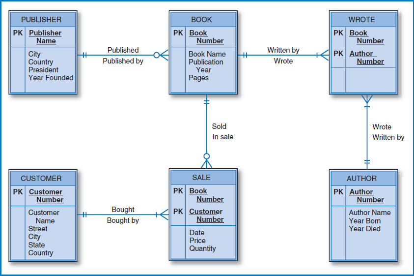
FIGURE 7.20 Good Reading Bookstores entity-relationship diagram

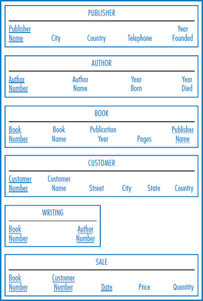
FIGURE 7.21 The Good Reading Bookstores relational database

Designing the World Music Association Database

Looking at the World Music Association E-R diagram in Figure 7.22, it appears that the orchestra entity would be a good central starting point for the database design process. Thus, the relational database in Figure 7.23 begins with the ORCHESTRA table. The Orchestra Name foreign key in the MUSICIAN table reflects the one-to-many relationship from orchestra to musician. Since degree is a dependent entity of musician in a one-to-many relationship and degrees (e.g. B.A.) are unique only within a musician, not only does Musician Number appear as a foreign key in the DEGREE table but also it must be part of that table's primary key. A similar situation exists between the composer and composition entities, as shown in the COMPOSER and COMPOSITION tables in the database. Finally, the many-to-many relationship between orchestra and composition is converted into the RECORDING table. Notice that the primary key of the RECORDING table begins with the Orchestra Name attribute and then continues with both the Composition Name and Composer Name attributes. This is because the primary key of one of the two entities in the many-to-many relationship, composition, is the combination of those two latter attributes.

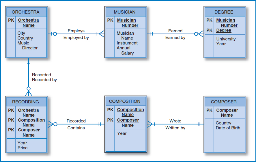
FIGURE 7.22 World Music Association entity-relationship diagram

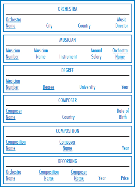
FIGURE 7.23 The World Music Association relational database

Designing the Lucky Rent-A-Car Database

Figure 7.24 shows the Lucky Rent-A-Car E-R diagram. The conversion to a relational database structure begins with the car entity and its four attributes, as shown in the CAR table of the database in Figure 7.25. Because car is on the “many side” of a one-to-many relationship with the manufacturer entity, the CAR table also has the Manufacturer Name attribute as a foreign key. The straightforward one-to-many relationship from car to maintenance event produces a MAINTENANCE EVENT table with Car Serial Number as a foreign key. The customer entity converts to the CUSTOMER table with its four attributes. The many-to-many relationship between car and customer converts to the RENTAL table. Car Serial Number, the unique identifier of the car entity, and Customer Number, the unique identifier of the customer entity, plus the Rental Date intersection data attribute form the three-attribute primary key of the RENTAL table, with Return Date and Total Cost as additional intersection data attributes. Rental Date has to be part of the primary key to achieve uniqueness because a particular customer may have rented a particular car on several different dates.

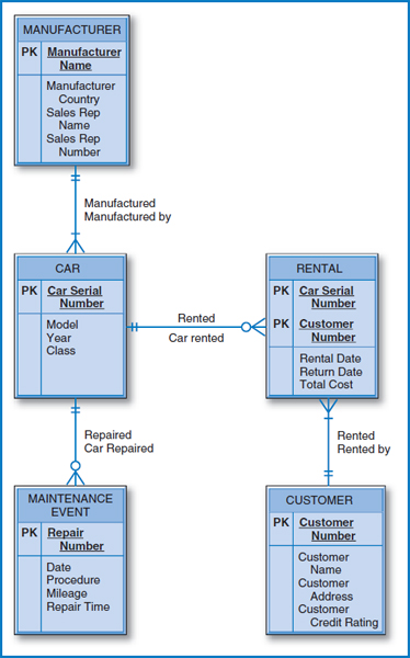
FIGURE 7.24 Lucky Rent-A-Car entity-relationship diagram

THE DATA NORMALIZATION PROCESS

Data normalization was the earliest formalized database design technique and at one time was the starting point for logical database design. Today, with the popularity of the Entity-Relationship model and other such diagramming tools and the ability to convert its diagrams to database structures, data normalization is used more as a check on database structures produced from E-R diagrams than as a full-scale database design technique. That's one of the reasons for learning about data normalization. Another reason is that the data normalization process is another way of demonstrating and learning about such important topics as data redundancy, foreign keys, and other ideas that are so central to a solid understanding of database management.

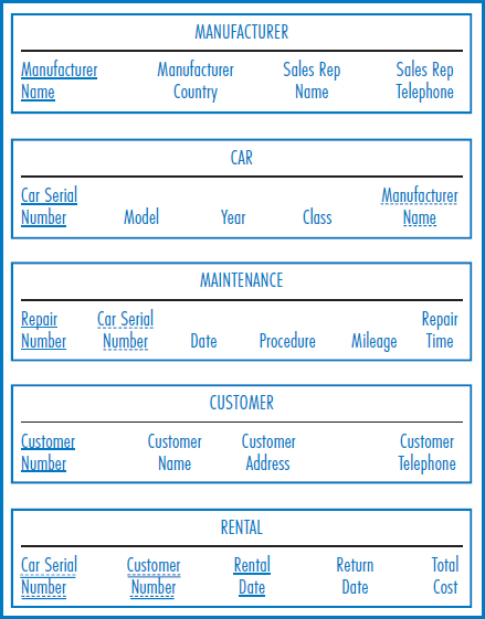
FIGURE 7.25 The Lucky Rent-A-Car relational database

Data normalization is a methodology for organizing attributes into tables so that redundancy among the non-key attributes is eliminated. Each of the resultant tables deals with a single data focus, which is just another way of saying that each resultant table will describe a single entity type or a single many-to-many relationship. Furthermore, foreign keys will appear exactly where they are needed. In other words, the output of the data normalization process is a properly structured relational database.

Introduction to the Data Normalization Technique

The input required by the data normalization process has two parts. One is a list of all the attributes that must be incorporated into the database: that is, all of the attributes in all of the entities involved in the business environment under discussion plus all of the intersection data attributes in all of the many-to-many relationships between these entities. The other input, informally, is a list of all of the defining associations among the attributes. Formally, these defining associations are known as functional dependencies. And what are defining associations or functional dependencies? They are a means of expressing that the value of one particular attribute is associated with a specific single value of another attribute. If we know that one of these attributes has a particular value, then the other attribute must have some other value. For example, for a particular Salesperson Number, 137, there is exactly one Salesperson Name, Baker, associated with it. Why is this true? In this example, a Salesperson Number uniquely identifies a salesperson and, after all, a person can have only one name! And this is true for every person! Informally, we might say that Salesperson Number defines Salesperson Name. If I give you a Salesperson Number, you can give me back the one and only name that goes with it. (It's a little like the concept of independent and dependent variables in mathematics. Take a value of the independent variable, plug it into the formula and you get back the specific value of the dependent variable associated with that independent variable.) These defining associations are commonly written with a right-pointing arrow like this:

In the more formal terms of functional dependencies, Salesperson Number, in general the attribute on the left side, is referred to as the determinant. Why? Because its value determines the value of the attribute on the right side. Conversely, we also say that the attribute on the right is functionally dependent on the attribute on the left.

Data normalization is best explained with an example and this is a good place to start one. In order to demonstrate the main points of the data normalization process, we will modify part of the General Hardware Co. business environment and focus on the salesperson and product entities. Let's assume that salespersons are organized into departments and each department has a manager who is not herself a salesperson. Then the list of attributes we will consider is shown in Figure 7.26. The list of defining associations or functional dependencies is shown in Figure 7.27.

Notice a couple of fine points about the list of defining associations in Figure 7.27. The last association:

shows that the combination of two or more attributes may possibly define another attribute. That is, the combination of a particular Salesperson Number and a particular Product Number defines or specifies a particular Quantity. Put another way, in this business context, we know how many units of a particular product a particular salesperson has sold. Another point, which will be important in demonstrating one step of the data normalization process, is that Manager Name is defined, independently, by two different attributes: Salesperson Number and Department Number:

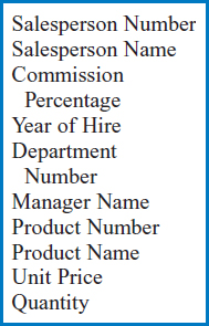
FIGURE 7.26 List of attributes for salespersons and products

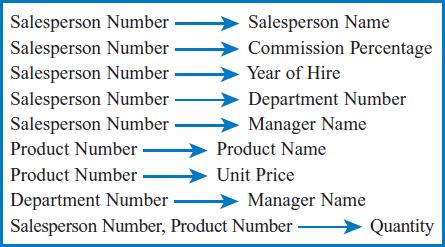
FIGURE 7.27 List of defining associations (functional dependencies) for the attributes of salespersons and products

Both these defining associations are true! If I identify a salesperson by his Salesperson Number, you can tell me who his manager is. Also, if I state a department number, you can tell me who the manager of the department is. How did we wind up with two different ways to define the same attribute? Very easily! It simply means that during the systems analysis process, both these equally true defining associations were discovered and noted. By the way, the fact that I know the department that a salesperson works in:

(and that each of these two attributes independently define Manager Name) will also be an issue in the data normalization process. More about this later.

Steps in the Data Normalization Process

The data normalization process is known as a “decomposition process.” Basically, we are going to line up all the attributes that will be included in the relational database and start subdividing them into groups that will eventually form the database's tables. Thus, we are going to “decompose” the original list of all of the attributes into subgroups. To do this, we are going to step through a number of normal forms. First, we will demonstrate what unnormalized data looks like. After all, if data can exist in several different normal forms, then there should be the possibility that data is in none of the normal forms, too! Then we will basically work through the three main normal forms in order:

• First Normal Form
• Second Normal Form
• Third Normal Form

There arc certain “exception conditions” that have also been described as normal forms. These include the Boyce-Codd Normal Form, Fourth Normal Form, and Fifth Normal Form. They are less common in practice and will not be covered here.

Here are three additional points to remember:

1. Once the attributes are arranged in third normal form (and if none of the exception conditions are present), the group of tables that they comprise is, in fact, a well-structured relational database with no data redundancy.
2. A group of tables is said to be in a particular normal form if every table in the group is in that normal form.
3. The data normalization process is progressive. If a group of tables is in second normal form it is also in first normal form. If they are in third normal form they are also in second normal form.

Unnormalized Data Figure 7.28 shows the salesperson and product-related attributes listed in Figure 7.26 arranged in a table with sample data. The salesperson and product data is taken from the General Hardware Co. relational database of Figure 5.14, with the addition of Department Number and Manager Name data. Note that salespersons 137, 204, and 361 are all in department number 73 and their manager is Scott. Salesperson 186 is in department number 59 and his manager is Lopez.

The table in Figure 7.28 is unnormalized. The table has four records, one for each salesperson. But, since each salesperson has sold several products and there is only one record for each salesperson, several attributes of each record must have multiple values. For example, the record for salesperson 137 has three product numbers, 19440, 24013, and 26722, in its Product Number attribute, because salesperson 137 has sold all three of those products. Having such multivalued attributes is not permitted in first normal form, and so this table is unnormalized.

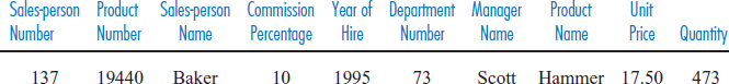
First Normal Form The table in Figure 7.29 is the first normal form representation of the data. The attributes under consideration have been listed out in one table and a primary key has been established. As the sample data of Figure 7.30 shows, the number of records has been increased(over the unnormalized representation) so that every attribute of every record has just one value. The multivalued attributes of Figure 7.28 have been eliminated. Indeed, the definition of first normal form is a table in which every attribute value is atomic, that is, no attribute is multivalued.

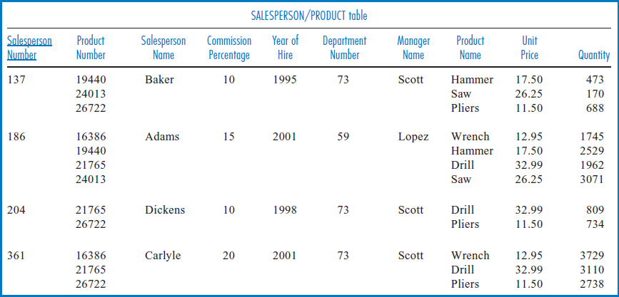
FIGURE 7.28 The salesperson and product attributes, unnormalized with sample data

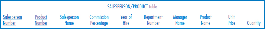
FIGURE 7.29 The salesperson and product attributes in first normal form

The combination of the Salesperson Number and Product Number attributes constitutes the primary key of this table. What makes this combination of attributes a legitimate primary key? First of all, the business context tells us that the combination of the two provides unique identifiers for the records of the table and that there is no single attribute that will do the job. That, of course, is how we have been approaching primary keys all along. Secondly, in terms of data normalization, according to the list of defining associations or functional dependencies of Figure 7.27, every attribute in the table is either part of the primary key or is defined by one or both attributes of the primary key. Salesperson Name, Commission Percentage, Year of Hire, Department Number, and Manager Name are each defined by Salesperson Number. Product Name and Unit Price are each defined by Product Number. Quantity is defined by the combination of Salesperson Number and Product Number.

Are these two different ways of approaching the primary key selection equivalent? Yes! If the combination of a particular Salesperson Number and a particular Product Number is unique, then it identifies exactly one record of the table. And, if it identifies exactly one record of the table, then that record shows the single value of each of the non-key attributes that is associated with the unique combination of the key attributes.

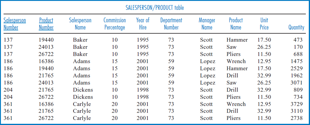
FIGURE 7.30 The salesperson and product attributes in first normal form with sample data

But that is the same thing as saying that each of the non-key attributes is defined by or is functionally dependent on the primary key! For example, consider the first record of the table in Figure 7.30.

The combination of Salesperson Number 137 and Product Number 19440 is unique. There is only one record in the table that can have that combination of Salesperson Number and Product Number values. Therefore, if someone specifies those values, the only Salesperson Name that can be associated with them is Baker, the only Commission Percentage is 10, and so forth. But that has the same effect as the concept of functional dependency. Since Salesperson Name is functionally dependent on Salesperson Number, given a particular Salesperson Number, say 137, there can be only one Salesperson Name associated with it, Baker. Since Commission Percentage is functionally dependent on Salesperson Number, given a particular Salesperson Number, say 137, there can be only one Commission Percentage associated with it, 10. And so forth.

First normal form is merely a starting point in the normalization process. As can immediately be seen from Figure 7.30, there is a great deal of data redundancy in first normal form. There are three records involving salesperson 137 (the first three records) and so there are three places in which his name is listed as Baker, his commission percentage is listed as 10, and so on. Similarly, there are two records involving product 19440 (the first and fifth records) and this product's name is listed twice as Hammer and its unit price is listed twice as 17.50. Intuitively, the reason for this is that attributes of two different kinds of entities, salespersons and products, have been mixed together in one table.

Second Normal Form Since data normalization is a decomposition process, the next step will be to decompose the table of Figure 7.29 into smaller tables to eliminate some of its data redundancy. And, since we have established that at least some of the redundancy is due to mixing together attributes about salespersons and attributes about products, it seems reasonable to want to separate them out at this stage. Informally, what we are going to do is to look at each of the non-key attributes of the table in Figure 7.29 and, on the basis of the defining associations of Figure 7.27, decide which attributes of the key are really needed to define it. For example, Salesperson Name really only needs Salesperson Number to define it; it does not need Product Number. Product Name needs only Product Number to define it; it does not need Salesperson Number. Quantity indeed needs both attributes, according to the last defining association of Figure 7.27.

More formally, second normal form, which is what we are heading for, does not allow partial functional dependencies. That is, in a table in second normal form, every non-key attribute must be fully functionally dependent on the entire key of that table. In plain language, a non-key attribute cannot depend on only part of the key, in the way that Salesperson Name, Product Name, and most of the other non-key attributes of Figure 7.29 do.

Figure 7.31 shows the salesperson and product attributes arranged in second normal form. There is a SALESPERSON Table in which Salesperson Number is the sole primary key attribute. Every non-key attribute of the table is fully defined just by Salesperson Number, as can be verified in Figure 7.27. Similarly, the PRODUCT Table has Product Number as its sole primary key attribute and the non-key attributes of the table are dependent just on it. The QUANTITY Table has the combination of Salesperson Number and Product Number as its primary key because its non-key attribute, Quantity, requires both of them together to define it, as indicated in the last defining association of Figure 7.27.

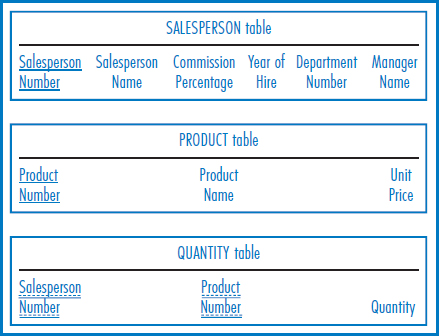
FIGURE 7.31 The salesperson and product attributes in second normal form

Figure 7.32 shows the sample salesperson and product data arranged in the second normal form structure of Figure 7.31. Indeed, much of the data redundancy visible in Figure 7.30 has been eliminated. Now, only once is salesperson 137's name listed as Baker, his commission percentage listed as 10, and so forth. Only once is product 19440's name listed as Hammer and its unit price listed as 17.50.

Second normal form is thus a great improvement over first normal form. But, has all of the redundancy been eliminated? In general, that depends on the particular list of attributes and defining associations. It is possible, and in practice it is often the case, that second normal form is completely free of data redundancy. In such a case, the second normal form representation is identical to the third normal form representation.

A close look at the sample data of Figure 7.32 reveals that the second normal form structure of Figure 7.31 has not eliminated all the data redundancy. At the right-hand end of the SALESPERSON Table, the fact that Scott is the manager of department 73 is repeated three times and this certainly constitutes redundant data. How could this have happened? Aren't all the non-key attributes fully functionally dependent on Salesperson Number? They are, but that is not the nature of the problem. It's true that Salesperson Number defines both Department Number and Manager Name and that's reasonable. If I'm focusing in on a particular salesperson, I should know what department she is in and what her manager's name is. But, as indicated in the next-to-last defining association of Figure 7.27, one of those two attributes defines the other: given a department number, I can tell you who the manager of that department is. In the SALESPERSON Table, one of the non-key attributes, Department Number, defines another one of the non-key attributes, Manager Name. This is what is causing the problem.

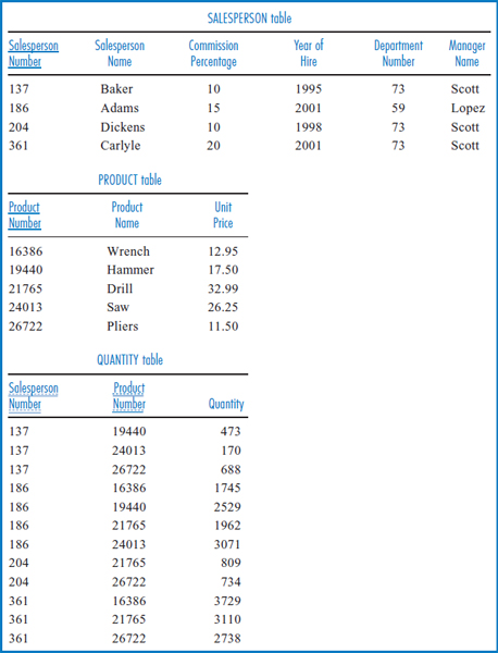
FIGURE 7.32 The salesperson and product attributes in second normal form with sample data

Third Normal Form In third normal form, non-key attributes are not allowed to define other non-key attributes. Stated more formally, third normal form does not allow transitive dependencies in which one non-key attribute is functionally dependent on another.

Again, there is one example of this in the second normal form representation in Figure 7.31. In the SALESPERSON table, Department Number and Manager Name are both non-key attributes and, as shown in the next-to-last association in Figure 7.27, Department Number defines Manager Name. Figure 7.33 shows the third normal form representation of the attributes. Note that the SALESPERSON Table of Figure 7.31 has been further decomposed into the SALESPERSON and DEPARTMENT Tables of Figure 7.33. The Department Number and Department Manager attributes, which were the problem, were split off to form the DEPARTMENT Table, but a copy of the Department Number attribute (the primary key attribute of the new DEPARTMENT Table) was left behind in the SALESPERSON Table. If this had not been done, there no longer would have been a way to indicate which department each salesperson is in.

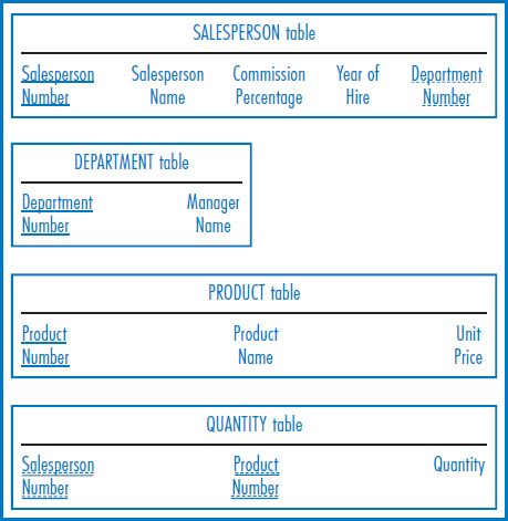
FIGURE 7.33 The salesperson and product attributes in third normal form

The sample data for the third normal form structure of Figure 7.33 is shown in Figure 7.34. Now, the fact that Scott is the manager of department 73 is shown only once, in the second record of the DEPARTMENT Table. Notice that the Department Number attribute in the SALESPERSON Table continues to indicate which department a salesperson is in.

There are several important points to note about the third normal form structure of Figure 7.33:

1. It is completely free of data redundancy.
2. All foreign keys appear where needed to logically tie together related tables.
3. It is the same structure that would have been derived from a properly drawn entity-relationship diagram of the same business environment.

Finally, there is one exception to the rule that in third normal form, non-key attributes are not allowed to define other non-key attributes. The rule does not hold if the defining non-key attribute is a candidate key of the table. Let's say, just for the sake of argument here, that the Salesperson Name attribute is unique. That makes Salesperson Name a candidate key in Figure 7.33's SALESPERSON Table. But, if Salesperson Name is unique, then it must define Commission Percentage, Year of Hire, and Department Number just as the unique Salesperson Number attribute does. Since it was not chosen to be the primary key of the table, Salesperson Name is technically a non-key attribute that defines other non-key attributes. Yet it does not appear from the sample data of Figure 7.34 to be causing any data redundancy problems. Since it was a candidate key, its defining other non-key attributes is not a problem.

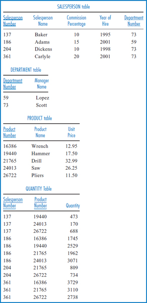
FIGURE 7.34 The salesperson and product attributes in third normal form with sample data

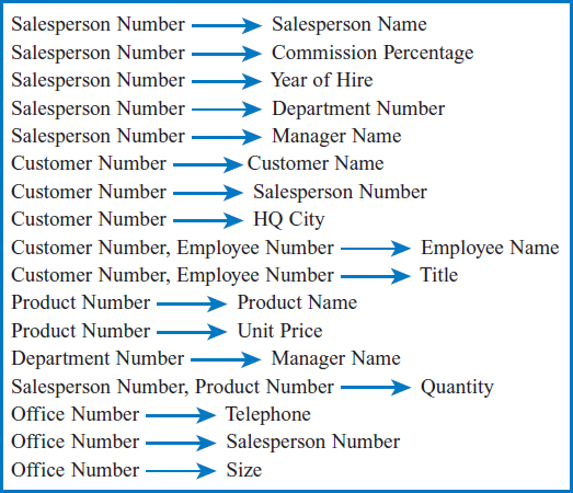
FIGURE 7.35 List of defining associations (functional dependencies) for the attributes of the General Hardware Company example

Example: General Hardware Co.

If the entire General Hardware Co. example, including the newly added Department Number and Manager Name attributes, were organized for the data normalization process, the list of defining associations or functional dependencies of Figure 7.27 would be expanded to look like Figure 7.35. Several additional interesting functional dependencies in this expanded list are worth pointing out. First, although Salesperson Number is a determinant, defining several other attributes, it is in turn functionally dependent on another attribute, Customer Number:

As we have already established, this functional dependency makes perfect sense. Given a particular customer, I can tell you who the salesperson is who is responsible for that customer. This is part of the one-to-many relationship between salespersons and customers. The fact that, in the reverse direction, a particular salesperson has several customers associated with him makes no difference in this functional dependency analysis. Also, the fact that Salesperson Number is itself a determinant, defining several other attributes, does not matter. Next:

Remember that in the General Hardware business environment, employee numbers are unique only within a customer company. Thus, this functional dependency correctly shows that the combination of the Customer Number and Employee Number attributes is required to define the Employee Name and Title attributes.

Figure 7.36 shows the General Hardware Co. attributes, including the added Department Number and Manager Name attributes, arranged in first normal form. Moving to second normal form would produce the database structure in Figure 7.19, except that the Department Number and Manager Name attributes would be split out in moving from second to third normal form, as previously shown.

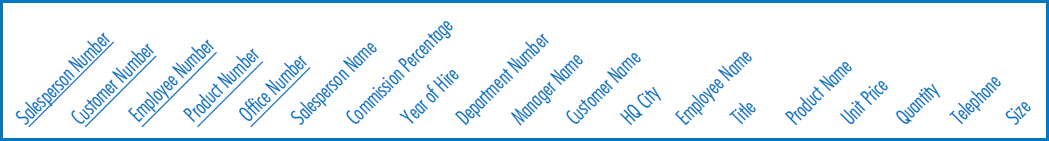
FIGURE 7.36 The General Hardware Company attributes in first normal form

Example: Good Reading Bookstores

In the General Hardware Co. example, the reason that the table representing the many-to-many relationship between salespersons and products

fell out so easily in the data normalization process was because of the presence of the functional dependency needed to define the intersection data attribute, Quantity:

A new twist in the Good Reading Bookstores example is the presence of the many-to-many relationship between the book and author entities with no intersection data. This is shown in the WRITING Table of Figure 7.21. The issue is how to show this in a functional dependencies list. There are a couple of possibilities. One is to show the two attributes defining “null”:

The other is to show paired “multivalued dependencies” in which the attribute on the left determines a list of attribute values on the right, instead of the usual single attribute value on the right. A double-headed arrow is used for this purpose:

These literally say that given a book number, a list of authors of the book can be produced and that given an author number, a list of the books that an author has written or co-written can be produced. In either of the two possibilities shown, the null and the paired multivalued dependencies, the notation in the functional dependency list can be used as a signal to split the attributes off into a separate table in moving from first to second normal form.

The other interesting point in the Good Reading Bookstores example involves the many-to-many relationship of the SALE Table in Figure 7.21. Recall that Date and Price were intersection data attributes that, because of the requirements of the company, had to be part of the primary key of the table. This would be handled very simply and naturally with a functional dependency that looks like this:

The complete list of functional dependencies is shown in Figure 7.37. First normal form for the Good Reading Bookstores example would consist of the list of its attributes with the following attributes in the primary key:

• Publisher Name
• Author Number
• Book Number
• Customer Number
• Date.

Moving from first to second normal form, including incorporating the rule described above for the many-to-many relationship with no intersection data, would directly yield the tables of Figure 7.21. As there are no instances of a non-key attribute defining another non-key attribute, this arrangement is already in third normal form.

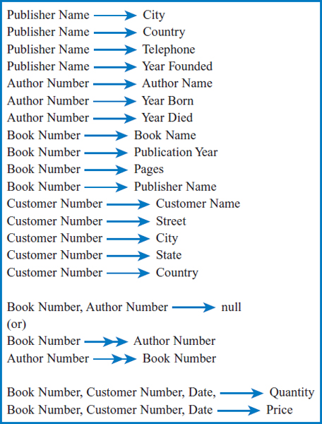
FIGURE 7.37 List of defining associations (functional dependencies) for the attributes of the Good Reading Bookstores example

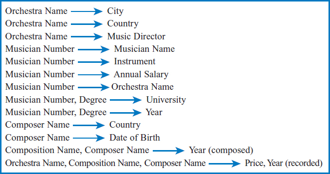
FIGURE 7.38 List of defining associations (functional dependencies) for the attributes of the World Music Association example

Example: World Music Association

The World Music Association example is straightforward in terms of data normalization. The complete list of functional dependencies is shown in Figure 7.38. Since degree is unique only within a musician and composition name is unique only within a composer, note that three of the functional dependencies are:

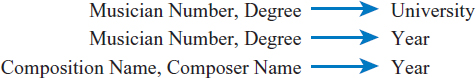
The primary key attributes in first normal form are:

• Orchestra Name
• Musician Number
• Degree
• Composer Name
• Composition Name

With this in mind, proceeding from first to second normal form will produce the tables in Figure 7.23. These are free of data redundancy and are, indeed, also in third normal form.

Example: Lucky Rent-A-Car

Figure 7.39 lists the Lucky Rent-A-Car functional dependencies. The primary key attributes in first normal form are:

• Manufacturer Name
• Car Serial Number
• Repair Number
• Customer Number
• Rental Date

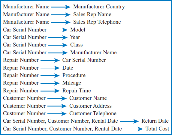
FIGURE 7.39 List of defining associations (functional dependencies) for the attributes of the Lucky Rent-A-Car example

Once again, the conversion from first to second normal form results in a redundancy-free structure, Figure 7.25, that is already in third normal form.

TESTING TABLES CONVERTED FROM E-R DIAGRAMS WITH DATA NORMALIZATION

As we said earlier, logical database design is generally performed today by converting entity-relationship diagrams to relational tables and then checking those tables against the data normalization technique rules. Since we already know that the databases in Figures 7.19, 7.21, 7.23, and 7.25 (for the four example business environments we've been working) with are in third normal form, there really isn't much to check. As one example, consider the General Hardware Co. database of Figure 7.19.

The basic idea in checking the structural worthiness of relational tables with the data normalization rules is to:

1. Check to see if there are any partial functional dependencies. That is, check whether any non-key attributes are dependent on or are defined by only part of the table's primary key.
2. Check to see if there are any transitive dependencies. That is, check whether any non-key attributes are dependent on or are defined by any other non-key attributes (other than candidate keys).

Both of these can be verified by the business environment's list of defining associations or functional dependencies.

In the SALESPERSON Table of Figure 7.19, there is only one attribute, Salesperson Number, in the primary key. Therefore there cannot be any partial functional dependencies. By their very definition, partial functional dependencies require the presence of more than one attribute in the primary key, so that a non-key attribute can be dependent on only part of the key! As for transitive dependencies, are any non-key attributes determined by any other non-key attributes? No! And, even if Salesperson Name is assumed to be a unique attribute and therefore it defines Commission Percentage and Year of Hire, this would be an allowable exception because Salesperson Name, being unique, would be a candidate key. The same analysis can be made for the other General Hardware tables with single-attribute primary keys: the CUSTOMER, PRODUCT, and OFFICE tables of Figure 7.19.

Figure 7.19's CUSTOMER EMPLOYEE Table has a two-attribute primary key because Employee Number is unique only within a customer. But then, by the very same logic, the non-key attributes Employee Name and Title must be dependent on the entire key, because that is the only way to uniquely identify who we are talking about when we want to know a person's name or title. Analyzing this further, Employee Name cannot be dependent on Employee Number alone because it is not a unique attribute. Functional dependency requires uniqueness from the determining side. And, obviously, Employee Name cannot be dependent on Customer Number alone. A customer company has lots of employees, not just one. Therefore, Employee Name and Title must be dependent on the entire primary key and the rule about no partial functional dependencies is satisfied. Since the non-key attributes Employee Name and Title do not define each other, the rule about no transitive dependencies is also satisfied and thus the table is clearly in third normal form.

In the SALES Table of Figure 7.19, there is a two-attribute primary key and only one non-key attribute. This table exists to represent the many-to-many relationship between salespersons and products. The non-key attributes, just Quantity in this case, constitute intersection data. By the definition of intersection data these non-key attributes must be dependent on the entire primary key. In any case, there would be a line in the functional dependency list indicating that Quantity is dependent on the combination of the two key attributes. Thus, there are no partial functional dependencies in this table. Interestingly, since there is only one non-key attribute, transitive dependencies cannot exist. After all, there must be at least two non-key attributes in a table for one non-key attribute to be dependent on another.

BUILDING THE DATA STRUCTURE WITH SQL

SQL has data definition commands that allow you to take the database structure you just learned how to design with the logical database design techniques and implement it for use with a relational DBMS. This process begins by the creation of “base tables.” These are the actual physical tables in which the data will be stored on the disk. The command that creates base tables and tells the system what attributes will be in them is called the CREATE TABLE command. Using the CREATE TABLE command, you can also specify which attribute is the primary key. As an example, here is the command to create the General Hardware Company SALESPERSON table we have been working with shown in Figure 7.19. (Note that the syntax of these commands varies somewhat among the various relational DBMS products on the market. The commands shown in this chapter, which are based on the ORACLE DBMS, are designed to give you a general idea of the command structures. You should check the specific syntax required by the DBMS you are using.)

CREATE TABLE SALESPERSON
(SPNUM CHAR(3) PRIMARY KEY,
SPNAME CHAR(12)
COMMPERCT DECIMAL(3,0)
YEARHIRE CHAR(4)
OFFNUM CHAR(3));

Notice that the CREATE TABLE command names the table SALESPERSON and lists the attributes in it (with abbreviated attribute names that we have created for brevity). Each attribute is given an attribute type and length. So SPNUM, the Salesperson Number, is specified as CHAR(3). It is three characters long (yes, it's a number, but it's not subject to calculations so it's more convenient to specify it as a character attribute). On the other hand, COMMPERCT, the Commission Percentage, is specified as DECIMAL(3,0), meaning that it is a three-position number with no decimal positions. Thus it could be a whole number from 0-999, although we know that it will always be a whole number from 0-100 since it represents a commission percentage. Finally, the command indicates that SPNUM will be the primary key of the table.

If a table in the database has to be discarded, the command is the DROP TABLE command.

DROP TABLE SALESPERSON;

A logical view (sometimes just called a “view”) is derived from one or more base tables. A view may consist of a subset of the columns of a single table, a subset of the rows of a single table, or both. It can also be the join of two or more base tables. The creation of a view in SQL does not entail the physical duplication of data in a base table into a new table. Instead, the view is a mapping onto the base table(s). It's literally a “view” of some part of the physical, stored data. Views are built using the CREATE VIEW command. Within this command, you specify the base table(s) on which the view is to be based and the attributes and rows of the table(s) that are to be included in the view. Interestingly, these specifications are made within the CREATE VIEW command using the SELECT statement, which is also used for data retrieval.

For example, to give someone access to only the Salesperson Number, Salesperson Name, and Year of Hire attributes of the SALESPERSON table, you would specify:

CREATE VIEW EMPLOYEE AS
SELECT SPNUM, SPNAME, YEARHIRE
FROM SALESPERSON;

The name of the view is EMPLOYEE, which can then be used in other SQL commands as if it were a table name. People using EMPLOYEE as a table name would have access to the Salesperson Number, Salesperson Name, and Year of Hire attributes of the SALESPERSON table but would not have access to the Commission Percentage or Office Number attributes (in fact, they would not even know that these two attributes exist!).

Views can be discarded using the DROP VIEW command:

DROP VIEW EMPLOYEE;

MANIPULATING THE DATA WITH SQL

Once the tables have been created, the focus changes to the standard data manipulation operations of updating existing data, inserting new rows in tables, and deleting existing rows in tables. (Data retrieval is discussed in Chapter 4.) The commands are UPDATE, INSERT, and DELETE. In the UPDATE command, you have to identify which row(s) of a table are to be updated based on data values within those rows. Then you have to specify which columns are to be updated and what the new data values of those columns in those rows will be. For example, consider the SALESPERSON table in Figure 7.34. If salesperson 204's commission percentage has to be changed from the current 10 percent to 12 percent, the command would be:

UPDATE SALESPERSON
SET COMMPERCT = 12
WHERE SPNUM = ‘204’;

Notice that the command first specifies the table to be updated in the UPDATE clause, then specifies the new data in the SET clause, then specifies the affected row(s) in the WHERE clause.

In the INSERT command, you have to specify a row of data to enter into a table. To add a new salesperson into the SALESPERSON table whose salesperson number is 489, name is Quinlan, commission percentage is 15, year of hire is 2011, and department number is 59, the command would be:

INSERT INTO SALESPERSON
VALUES
(‘489’,‘Quinlan’,15,‘2011’,‘59’);

In the DELETE command you have to specify which row(s) of a table are to be deleted based on data values within those rows. To delete the row for salesperson 186 the command would be:

DELETE FROM SALESPERSON
WHERE SPNUM = ‘186’;

SUMMARY

Logical database design is the process of creating a database structure that is free of data redundancy and that promotes data integration. There are two techniques for logical database design. One technique involves taking the entity-relationship diagram that describes the business environment and going through a series of steps to convert it to a well structured relational database structure. The other technique is the data normalization technique. Furthermore, the data normalization technique can be used to check the results of the E-R diagram conversion for errors.

SQL is both a data definition language and a data manipulation language. Included in the basic data definition commands are CREATE TABLE, DROP TABLE, CREATE VIEW, AND DROP VIEW. Included in the basic data manipulation commands are UPDATE, INSERT, and DELETE.

KEY TERMS

CREATE TABLE

CREATE VIEW

Data normalization

Data structures

Database design

DELETE

DROP TABLE

DROP VIEW

Entity-relationship diagram conversion

First normal form

INSERT

Logical database design

Second normal form

Third normal form

UPDATE

QUESTIONS

1. What is logical database design?
2. What is physical database design and how does it relate to logical database design?
3. In general terms, describe the main logical database design techniques and how they relate to one another.
4. Based on an entity-relationship diagram, how can you determine how many tables there will be in the corresponding relational database?
5. Describe the process for converting entities in each of the following relationships into relational database structures:
   1. One-to-one binary relationship.
   2. One-to-many binary relationship.
   3. Many-to-many binary relationship.
   4. One-to-one unary relationship.
   5. One-to-many unary relationship.
   6. Many-to-many unary relationship.
   7. Ternary relationship.
6. Describe the data normalization process including its specific steps. Why is it referred to as a “decomposition process?”
7. Explain the following terms:
   1. Functional dependency.
   2. Determinant.
8. What characterizes unnormalized data? Why is such data problematic?
9. What characterizes tables in first normal form? Why is such data problematic?
10. What is a partial functional dependency? What does the term “fully functionally dependent” mean?
11. What is the rule for converting tables in first normal form to tables in second normal form?
12. What is the definition of data in second normal form?
13. What is a transitive dependency?
14. What is the rule for converting tables in second normal form to tables in third normal form?
15. What is the definition of data in third normal form?
16. What are the characteristics of data in third normal form?
17. How can data normalization be used to check the results of the E-R diagram-to-relational database conversion process?
18. What SQL command do you use to produce a new table structure? What SQL command do you use to discard a table?
19. What is a view? What SQL commands do you use to produce a new view and to discard one that is no longer needed?
20. What are the SQL data manipulation commands and what are their functions?

EXERCISES

1. Convert the Video Centers of Europe, Ltd., entity-relationship diagram in Exercise 2.2 into a well structured relational database.
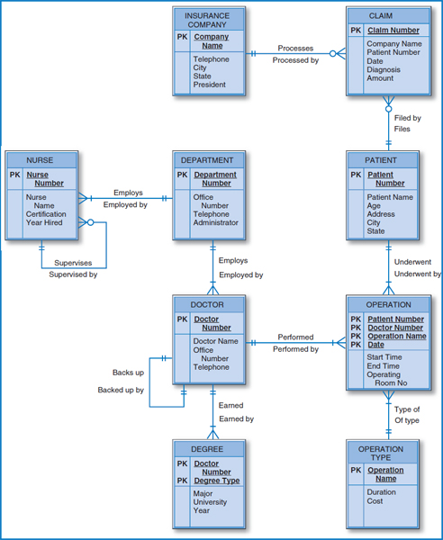
2. Convert the Central Hospital entity-relationship diagram on the next page into a well-structured relational database.
3. Video Centers of Europe, Ltd., is a chain of movie DVD rental stores. It must maintain data on the DVDs it has for rent, the movies recorded on the DVDs, its customers, and the actual rental. Each DVD for rent has a unique serial number. Movie titles and customer numbers are also unique identifiers. Assume that each movie has exactly one “star.” Note the difference in the year that the movie was originally filmed and the date that a DVD—an actual disk—was manufactured. Some of the attributes and functional dependencies in this environment are as follows:
   • Attributes
   • DVD Number
   • Manufacture Date
   • Movie Title
   • Star
   • Year Filmed
   • Length [in minutes]
   • Customer Number
   • Customer Name
   • Customer Address
   • Rental Date
   • Return Date
   • Fee Paid

   Functional Dependencies

   

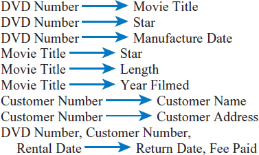
   For each of the following tables, first write the table's current normal form (as 1NF, 2 NF, or 3 NF). Then, take those tables that are currently in 1 NF or 2 NF and reconstruct them as well structured 3 NF tables. Primary key attributes are underlined. Do not assume any functional dependencies other than those shown.

   1. Movie Title, Star, Length, Year Filmed
   2. DVD Number, Customer Number, Rental Date, Customer Name, Return Date, Fee Paid
   3. DVD Number, Manufacture Date, Movie Title, Star
   4. Movie Title, Customer Number, Star, Length, Customer Name, Customer Address
   5. DVD Number, Customer Number, Rental Date, Return Date, Fee Paid
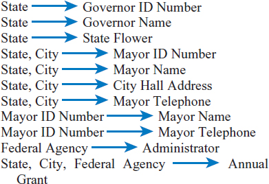
4. The U.S. government wants to keep track of information about states, governors, cities, and mayors. In addition, it wants to maintain data on the various federal agencies and the annual grants each agency gives to the individual states. Each federal agency is headed by an administrator. Agency names and state names are unique but city names are unique only within a state. The attributes and functional dependencies in this environment are as follows:
   • Attributes
   • State
   • Governor ID Number
   • Governor Name
   • State Flower
   • City
   • Mayor ID Number
   • Mayor Name
   • City Hall Address
   • Mayor Telephone
   • Federal Agency
   • Administrator
   • Annual Grant

   Functional Dependencies

   

   

   Central Hospital entity-relationship diagram

   For each of the following tables, first write the table's current normal form (as 1NF, 2NF, or 3NF). Then, reconstruct those tables that are currently in 1 NF or 2 NF as well structured 3 NF tables. Primary key attributes are underlined. Do not assume any functional dependencies other than those shown.

   1. State, City, Governor Name, Mayor ID Number, Mayor Name, Mayor Telephone
   2. State, City, Mayor Name, Mayor Telephone
   3. State, City, Federal Agency, Governor Name, Administrator, Annual Grant
   4. State, City, Governor Name, State Flower, Mayor Telephone
   5. State, City, City Hall Address, Mayor ID Number, Mayor Name, Mayor Telephone
5. Consider the General Hardware relational database shown in Figure 7.19.
   1. Write an SQL command to create the CUSTOMER table.
   2. Write an SQL command to create a view of the CUSTOMER table that includes only the Customer Number and HQ City attributes.
   3. Write an SQL command to discard the OFFICE table.
   4. Assume that Customer Number 8429 is the responsibility of Salesperson Number 758. Write an SQL command to change that responsibility to Salesperson Number 311.
   5. Write an SQL command to add a new record to the CUSTOMER table for Customer Number 9442. The Customer Name is Smith Hardware Stores, the responsible salesperson is Salesperson Number 577, and the HQ City is Chicago.

MINICASES

1. Happy Cruise Lines. Convert the Happy Cruise Lines entity-relationship diagram on the next page into a well structured relational database.
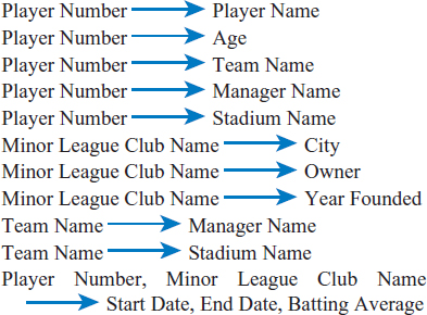
2. Super Baseball League. The Super Baseball League wants to keep track of information about its players, its teams, and the minor league teams (which we will call minor league “clubs” to avoid using the word “team” twice). Minor league clubs are not part of the Super Baseball League but players train in them with the hope of eventually advancing to a team in the Super Baseball League. The intent in this problem is to keep track only of the current team on which a player plays in the Super Baseball League. However, the minor league club data must be historic and include all of the minor league clubs for which a player has played. Team names, minor league club names, manager names, and stadium names are assumed to be unique, as, of course, is player number.

   Design a well structured relational database for this Super Baseball League environment using the data normalization technique. Progress from first to second normal form and then from second to third normal form justifying your design decisions at each step based on the rules of data normalization. The attributes and functional dependencies in this environment are as follows:

   • Attributes
   • Player Number
   • Player Name
   • Player Age
   • Team Name
   • Manager Name
   • Stadium Name
   • Minor League Club Name
   • Minor League Club City
   • Minor League Club Owner
   • Minor League Club Year Founded
   • Start Date
   • End Date
   • Batting Average

   Functional Dependencies

   

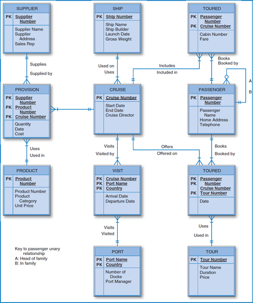
Happy Cruise Lines entity-relationship diagram