Chapter 5
Numerical Methods
Quantitative analyses are essential elements in solving forward and inverse problems. To utilize computers, we should devise numerically implementable algorithms to solve given problems, which include step-by-step procedures to obtain final answers. Formulation of a forward as well as an inverse problem should be done bearing in mind that we will adopt a certain numerical algorithm to solve them. After reviewing the basics of numerical computations, we will introduce various methods to solve a linear system of equations, which are most commonly used to obtain numerical solutions of both forward and inverse problems. Considering that most forward problems are formulated by using partial differential equations, we will study numerical techniques such as the finite difference method and finite element method. The accuracy or consistency of a numerical solution as well as the convergence and stability of an algorithm to obtain the solution need to be investigated.
5.1 Iterative Method for Nonlinear Problem
Recall the abstract form of the inverse problem in section 4.1, where we tried to reconstruct a material property P from knowledge of the input data X and output data Y using the forward problem (4.1). It is equivalent to the following root-finding problem:
![]()
where X and Y are given data.
We assume that both the material property P and F(P, X) are expressed as vectors in N-dimensional space ![]() . Imagine that P* is a root of G(P) = 0 and P0 is a reasonably good guess in the sense that P0 + ΔP = P* for a small perturbation ΔP. From the tangent line approximation, we can approximate
. Imagine that P* is a root of G(P) = 0 and P0 is a reasonably good guess in the sense that P0 + ΔP = P* for a small perturbation ΔP. From the tangent line approximation, we can approximate
![]()
where J(P0) denotes the Jacobian of G(P) at P0. Then, the solution P* = P0 + ΔP can be approximated by
![]()
The Newton–Raphson algorithm is based on the above idea, and we can start from a good initial guess P0 to perform the following recursive process:
The convergence of this approach is related to the condition number of the Jacobian matrix J(P*). If J(P*) is nearly singular, the root-finding problem G(P) = 0 is ill-posed. According to the fixed point theorem, the sequence Pn converges to a fixed point P* provided that Φ(P): = P − [J(P)]−1G(P) is a contraction mapping: for some 0 < α < 1,
To be precise, if Φ is a contraction mapping satisfying (5.2), then
![]()
Hence, {Pn} is a Cauchy sequence, which guarantees the convergence Pn → P*. Here, P* is a fixed point, Φ(P*) = P*. Owing to the convergence of the recursive process (5.1), we can compute an approximate solution of the root-finding problem G(P) = 0.
5.2 Numerical Computation of One-Dimensional Heat Equation
We begin with a simple problem of solving the following one-dimensional heat equation with the thermal diffusivity coefficient κ > 0:
To compute an approximate numerical solution of u(x, t) in (5.3), we discretize xt-space into a collection of grid points and express u in the following discrete form:
![]()
where Δx = 1/N and the superscript n and subscript k, respectively, specify the time step and the space step. The quantity ∂tu can be approximated by the first-order time derivative using a finite difference scheme of the two-point Euler difference:
![]()
where ∂tu|k, n = ∂tu(kΔx, nΔt).
The expressions for the space derivatives can be obtained by Taylor's expansion.
- Forward difference:
![]()
![]()
- Backward difference:
![]()
![]()
- Central difference:
![]()
Here, the “big O” notation ϕ(x) = O(η(x)) is used to describe the limiting behavior of the function ϕ such that
![]()
Using three-point central difference schemes to approximate the second-order space derivative, we get the following recurrence relations.
- Explicit scheme or forward Euler method:
 (the temperature at time n + 1 and position k) depends explicitly on
  at the previous time n using the relation
![]()
- Implicit scheme or backward Euler method: the Laplacian (∂2u/∂x2)|k, n+1 and
 at time n + 1 are evaluated from the implicit relation

- Crank–Nicolson scheme: we use the average of the explicit and implicit schemes

With the explicit scheme, the diffusion equation in (5.3) can be expressed as
Here, the last term can be viewed as the truncation error (or discretization error), which is the difference between the solution of the explicit scheme equation and the exact analytic solution.
5.6 ![]()
![]()
When using a specific computational scheme, we should check the following fundamental conditions.
- Convergence. Does the numerical solution
 converge to the true solution u?
 - Consistency. Does the discretization error go to zero as Δt, Δx → 0?
- Stability. Do small errors in the initial and boundary conditions cause small errors in the numerical solution?
5.2.1 Explicit Scheme
In the explicit scheme, it is easy to compute numerical solutions because it is explicit. However, computational experience shows that, depending on the size of κ(Δx)2/Δt, numerical errors (round-off and truncation errors) can be magnified as the iterative computations progress in time. It is well known that this explicit method requires ![]() in order to be numerically stable. Owing to this requirement, it is computationally expensive.
in order to be numerically stable. Owing to this requirement, it is computationally expensive.
If we substitute the approximations into ![]() and ignore the higher-order terms O(Δt) and O(Δx2), we obtain the following system of difference equations for interior grid points:
and ignore the higher-order terms O(Δt) and O(Δx2), we obtain the following system of difference equations for interior grid points:
![]()
This formation is called the explicit forward Euler method because the time derivative is represented with a forward Euler approximation. The solution at time t = nΔt can be solved explicitly as
or
where ![]() . Since u in (5.3) has homogeneous boundary conditions,
. Since u in (5.3) has homogeneous boundary conditions,
5.9 ![]()
From the above formula, we can directly compute un, an approximate solution u(x, Δt), from the discrete version of the initial condition u0 (a discrete form of u(x, 0) = f(x)). This step-by-step time advancing process (5.8) is called time marching since the unknown values un+1 at the next time n + 1 are directly computed from the computed values un at the previous time n. According to (5.4), the computed solution by the time marching scheme (5.8) can be O(Δt) accurate in time and O(Δx2) accurate in space.
We should note that the exact solution ![]() of the discretized problem (5.7) may not be an accurate approximate solution of the original continuous heat equation even if Δx and Δt are sufficiently small. The stability of a numerical scheme is closely associated with numerical errors. Hence, we need to check the error
of the discretized problem (5.7) may not be an accurate approximate solution of the original continuous heat equation even if Δx and Δt are sufficiently small. The stability of a numerical scheme is closely associated with numerical errors. Hence, we need to check the error ![]() between the numerical solution
between the numerical solution ![]() of the finite difference equation (5.7) and the true solution
of the finite difference equation (5.7) and the true solution ![]() , with u being the solution of the continuous equation (5.3). From (5.7) and (5.5), the error
, with u being the solution of the continuous equation (5.3). From (5.7) and (5.5), the error ![]() can be expressed as
can be expressed as
![]()
If ![]() , the error
, the error ![]() is estimated by
is estimated by
![]()
Since the above estimate holds for all k and n, we obtain
We should note that, as Δt → 0, ![]() . The estimate (5.10) shows that
. The estimate (5.10) shows that ![]() converges to the true solution u as Δt → 0 provided r < 0.5. The numerical errors are proportional to the time step and to the square of the space step. For details, please refer to Haberman (1987).
converges to the true solution u as Δt → 0 provided r < 0.5. The numerical errors are proportional to the time step and to the square of the space step. For details, please refer to Haberman (1987).
![]()

![]()

![]()

![]()
![]()
![]()
Unfortunately, the numerical solution is unstable when ![]() no matter how small Δx and Δt are. If
no matter how small Δx and Δt are. If ![]() , the error
, the error ![]() may grow with the time step n. This is the major shortcoming of the explicit method. Now, we present the Lax equivalence theorem (Lax and Richtmyer 1956), which plays an important role in determining the convergence of a solution of the finite difference method to a solution of the partial differential equation (PDE).
may grow with the time step n. This is the major shortcoming of the explicit method. Now, we present the Lax equivalence theorem (Lax and Richtmyer 1956), which plays an important role in determining the convergence of a solution of the finite difference method to a solution of the partial differential equation (PDE).
5.2.2 Implicit Scheme
The major shortcoming of the explicit method is the time step constraint Δt < [1/(2κ)]Δx2 to guarantee the stability so that the computed solution ![]() is a good approximation to the true solution u(xk, tn). Using the explicit scheme or forward Euler method, the numerical solution
is a good approximation to the true solution u(xk, tn). Using the explicit scheme or forward Euler method, the numerical solution ![]() may blow up if the time step does not satisfy the constraint Δt < [1/(2κ)]Δx2.
may blow up if the time step does not satisfy the constraint Δt < [1/(2κ)]Δx2.
We can remove the time step constraint Δt < [1/(2κ)]Δx2 of the forward Euler method by the use of the implicit scheme or backward Euler method:
where we evaluate the approximation for uxx at tn+1 = (n + 1)Δt rather than at tn. This implicit backward Euler method leads one to solve the following implicit linear system:
where

![]()
Since the matrix A in (5.12) is diagonally dominant, the implicit scheme is always numerically stable and convergent regardless of the choice of the time step. This is the major advantage of the implicit backward Euler method over the explicit forward Euler method (5.7). On the other hand, the implicit method requires a computation of the inverse matrix A at each time step and, therefore, it is computationally more intensive.
5.2.3 Crank–Nicolson Method
The Crank–Nicolson method combines the forward and backward Euler methods as
![]()
When ![]() , the scheme is called the Crank–Nicolson scheme.
, the scheme is called the Crank–Nicolson scheme.
We can summarize the following features.
- For β = 0, the scheme is explicit. It is stable under the condition Δt ≤ [1/(2κ)]Δx2. Owing to this constraint, the time step has to be chosen small enough.
- For β ≠ 0, the scheme is implicit. The scheme for β = 1 is unconditionally stable.
- When
 , the scheme is the Crank–Nicolson scheme, which is unconditionally stable.
5.3 Numerical Solution of Linear System of Equations
Finding a numerical solution of a forward problem and also an inverse problem often requires solving a system of linear algebraic equations,
![]()
for u. We can view a solution u of the system as a minimizer of the following functional:
![]()
Assuming that A is invertible, we consider a quantitative bound for the error in the computed solution of the linear system. We define the norm of the matrix A as
![]()
With u being the solution of Au = b and u + Δu being the solution of A[u + Δu] = b + Δb, we have

where cond(A) is called the condition number of the matrix A, indicating an amplification factor that bounds the maximum relative change in the solution due to a given relative change in the vector on the right-hand side.
5.3.1 Direct Method using LU Factorization
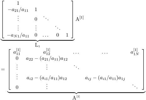
The most common direct method of solving Au = b is LU-factorization with forward and backward substitutions. By applying the Gaussian elimination process, we can express the matrix A as
![]()
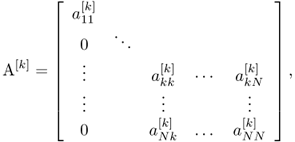
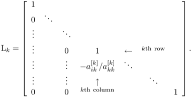
where L is a unit lower triangular matrix and U is an upper triangular matrix. We summarize the process to find L and U as follows:
 .
.
![]()
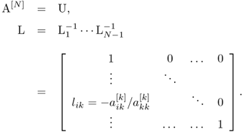
Given such an LU-factorization, we can solve the system Au = b via the forward and backward substitutions. Such direct methods are usually applied to the cases where the size of the matrix A is relatively small.
5.3.2 Iterative Method using Matrix Splitting
When the problem Au = b is too large, one may use an iterative method by generating a sequence un → u with a low computational cost. The most commonly used iterative methods for solving Au = b are based on the decomposition of the matrix A into two parts A = B + (A − B) so that the linear system Au = b can be rewritten as
![]()
Then, we set the iteration scheme as follows:
An iterative method expressed in the form of (5.13) is called the stationary iterative method. For the choice of B in the stationary iterative method, we use the decomposition
![]()
where D is the diagonal part of A and L and U are the lower and upper triangular matrices with zeros on their diagonals, respectively. The most common stationary iterative schemes are as follows.
- Jacobi method: with B = D and G = D−1(L + U), the iterative scheme is
![]()
- Damped Jacobi method: use G = (I − ωD−1A) with the damping factor ω to get the iterative scheme
![]()
- Gauss–Seidel method: use G = − (L + D)−1U to get
![]()
- Successive over-relaxation (SOR) method: use
 to get
![]()
Throughout this section, we assume that the stationary iterative scheme (5.13) is consistent with Au = b, that is,
From (5.13) and (5.14), we have
The above identity leads directly to the following theorem.
![]()
To be precise, assume that G has N linearly independent eigenvectors v1, …, vN with associated eigenvalues λ1, …, λN and that |λN| = ρ(G). Then, from (5.15), we have

and, therefore,
![]()
Hence, the spectral radius ρ(G) measures the speed of convergence when ρ(G) < 1.
![]()
![]()
![]()
The successive relaxation (SR) method is
![]()
The condition 0 < ω < 1 is called under-relaxation, whereas the condition ω > 1 is called over-relaxation. The choice of ω for faster convergence depends on the structure of A.
5.3.3 Iterative Method using Steepest Descent Minimization
Throughout this section, we assume that A is a real symmetric N × N matrix. We can iteratively solve Au = b by searching for a solution of the following equivalent minimization problem:
![]()
Then, Au = b if and only if
![]()
From the above equivalence relation, we have the following: if A is positive definite, then Au = b if and only if u minimizes the energy functional Φ(v). The minimum value of Φ is Φ(A-1b) = ![]() .
.

![]()
The steepest descent method to find u = A−1b is to search for a minimum point of Φ by traveling in the steepest descent direction of Φ. It is important to note that the residual vector r = b − Av associated with any vector v points in the steepest descent direction of Φ. Taking an iterative step in the steepest descent direction leads us to approach the minimum point u = A−1b. The following updating steps describe the general procedure:
![]()
For the convergence analysis of the steepest descent method, note that
![]()
Hence, (5.16) can be expressed as
5.17 ![]()
Denoting em: = um − u, (5.16) can be written as
For an intuitive understanding of the rate of convergence of the steepest descent method, we should note that the error em = um − u measures the difference in the domain space, whereas the residual rm = A(u − um) = − ∇Φ(um), indicating the steepest descent direction, measures the difference in the range space.
We can get a convergence analysis using eigenvectors v1, …, vN of A (assumed to be an orthonormal basis in ![]() ) with associated eigenvalues λ1, …, λN, ordered so that |λ1| ≤ ··· ≤ |λN|. Assume that
) with associated eigenvalues λ1, …, λN, ordered so that |λ1| ≤ ··· ≤ |λN|. Assume that
![]()
From (5.18), we have

where

Now, consider the following two special cases.
- In the special case of e0 = vj,
![]()
- If λ1 = ··· = λN, then
 and hence u1 is the exact solution.
The following exercise explains the rate of convergence of the steepest descent method.
![]()

![]()
The above exercise explains that the steepest descent method can converge very quickly when α ≈ 0. Note that α ≈ 0 if either λN/λ1 ≈ 1 or e0 is close to an eigenvector.
However, the rate of convergence would be very slow when |λN|/|λ1| is large. In the case where |λN|/|λ1| ≈ ∞, it is possible that the steepest descent direction rm from a given point um is very different from the direction pointing to the true solution u. The worst case is when e0 ≈ λNv1 + λ1vn, and this causes a sluggish performance of the steepest descent method in which the iterative scheme takes many short and inefficient switchbacks down to the valley floor. It may include steps with the same directions as those in earlier steps.
![]()
5.19 ![]()
![]()
![]()
![]()
![]()
5.20 ![]()
5.3.4 Conjugate Gradient (CG) Method
To deal with inefficient switchbacks in finding u = A−1b using the steepest descent method, the conjugate gradient (CG) method was proposed by choosing new search directions taking account of the progress in previous ones. Throughout this section, we assume that A is symmetric and positive definite. Two vectors v and w are conjugate with respect to A if they are A-orthogonal:
![]()
To understand the key idea of the CG method, we pick orthogonal search directions d0, d1, …, dN−1 and choose

Then, eN = 0 and uN must be the exact solution of Au = b. This procedure requires at most N steps to compute u provided that κm is computable. Unfortunately, we cannot compute uN since the computation of κm requires the unknown quantity u.
To deal with this problem, we use the fact that Aem is computable though em is not, and make the search direction A-orthogonal instead of orthogonal. Suppose that a1, …, aN−1 are A-orthogonal:
![]()
Our new requirement is that
![]()
It is crucial to observe that κm is computable as
![]()
Now, we need to determine the A-orthogonal basis set {a0, …, aN−1}. It is not desirable to use the Gram–Schmidt method since the process is roughly equivalent to performing Gaussian elimination. In the CG method, the search directions are constructed by conjugation of the residuals. We choose the search direction of the vector form
![]()
and hence
![]()
This choice makes sense for many reasons.
![]()

![]()
Now, we are ready to explain the basic CG algorithm. Let ![]() be symmetric and positive definite. The following algorithm solves Au = b starting with the initial guess u0:
be symmetric and positive definite. The following algorithm solves Au = b starting with the initial guess u0:
For detailed explanation for this method, see Allen et al. (1988). We may view the CG method as a method between the steepest descent and Newton's methods. Since each search direction pm is A-conjugate to all previous search directions, the CG algorithm requires at most N iterations to converge so that uN must be the exact solution from the theoretical point of view. However, in practice, when N is large, we need to take account of numerical round-off errors, and it is possible that the exact solution is never obtained.
Since the error em = u − um satisfies

the basic CG method may show poor performance for a large condition number ![]() . These observations motivated the use of a preconditioner. The idea is to replace
. These observations motivated the use of a preconditioner. The idea is to replace
![]()
where B−T is the transpose of B−1. To be precise, define G(x): = Φ(Bv) with x = Bv. Then, it is easy to see that
![]()
and
![]()
which is equivalent to
![]()
5.4 Finite Difference Method (FDM)
5.4.1 Poisson Equation
We examine numerical techniques to find a solution for the Poisson equation in a two-dimensional rectangular domain Ω = {(x, y):0 < x < a, 0 < y < b}:
The simplest way to solve (5.21) is to convert it to an equivalent system of difference equations using a finite difference approximation. Let Δx = a/m and Δy = b/n denote the step size in the x and y directions, respectively. Let
![]()
Let uk, j denote the computed value of u(xk, yj). To convert the Poisson equation uxx + uyy = f into a difference equation, we use finite difference approximations for the second derivatives. The three-point central difference approximations for the second derivatives are

Ignoring the higher-order terms, we get the following system of difference equations for the interior grid points:
where fk, j = f(xk, yj) and gk, j = g(xk, yj).
We often take the square grid as Δx = Δy = h. Then, we may conveniently write the structure of the five-point approximation in terms of the following stencil as

The problem of the system of difference equations can be written as the following linear system.
- Let u = [u1, 1, …, u1, n−1, u2, 1, …, um−1, n−1].
- Let A be the (m − 1)(n − 1) × (m − 1)(n − 1) square matrix:
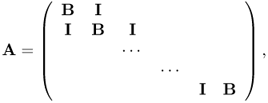
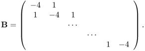
- The finite difference system (5.22) can be written as
5.23 ![]()
5.4.2 Elliptic Equation
Assume that Ω is a square region in ![]() . We will explain a discretized version of the elliptic equation:
. We will explain a discretized version of the elliptic equation:
![]()
We divide Ω uniformly into N × N subsquares Ωi, j with the center point (xi, yj), where i, j = 0, …, N − 1. We assume that the conductivity σ is constant on each subsquare Ωi, j, say σi, j:
![]()
The solution u can be approximated by a vector ![]() such that each interior voltage uk where k = i + jN is determined by the weighted average (depending on the conductivity σ) of the four neighboring potentials. To be precise, the conductivity equation ∇ · (σ∇u(r)) = 0 can be written in the following discretized form:
such that each interior voltage uk where k = i + jN is determined by the weighted average (depending on the conductivity σ) of the four neighboring potentials. To be precise, the conductivity equation ∇ · (σ∇u(r)) = 0 can be written in the following discretized form:
with
5.25 ![]()
where ![]() denote north, south, east and west neighboring points of the kth point. The discretized conductivity equation (5.24) with the Neumann boundary condition g can be written as a linear system Au = g, where g is the injection current vector associated with g.
denote north, south, east and west neighboring points of the kth point. The discretized conductivity equation (5.24) with the Neumann boundary condition g can be written as a linear system Au = g, where g is the injection current vector associated with g.
5.5 Finite Element Method (FEM)
The finite element method (FEM) is a useful tool to compute an approximate numerical solution of a PDE (Johnson 2009). This section summarizes the FEM to find an approximate solution of a PDE.
5.5.1 One-Dimensional Model
We explain Galerkin's method for solving the following elliptic equation as an example:
The weak form of (5.26) is
where ϕ satisfies ϕ(0) = 0. Galerkin's method discretizes the weak form (5.27). Let h = 1/N and define Vh as follows:
![]()
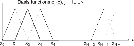
As shown in Figure 5.1, we choose ϕ1, …, ϕN ∈ Vh such that
![]()
Then, the finite element space is ![]() .
.
Figure 5.1 Basis functions
We look for an approximate solution
5.28 
Substituting ![]() into (5.27) yields
into (5.27) yields
The identity (5.29) can be written as the following matrix form:
5.30 ![]()
where A is an N × N matrix given by


The matrix A is sparse:
- If |i − j| > 1, then
 , and hence
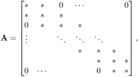
- If j − i = 1, then
 .
. - If i = j ≠ N, then
 .
. - If i = j = N, then
 .
.
5.5.2 Two-Dimensional Model
Let Ω be a domain in the two-dimensional space ![]() with smooth boundary ∂Ω and let σ be a positive bounded function in Ω. For a given
with smooth boundary ∂Ω and let σ be a positive bounded function in Ω. For a given ![]() , we consider the Neumann boundary value problem:
, we consider the Neumann boundary value problem:
We try to find an approximate solution of (5.31) within the set ![]() . The FEM uses the weak formulation for the solution u:
. The FEM uses the weak formulation for the solution u:
5.32 ![]()
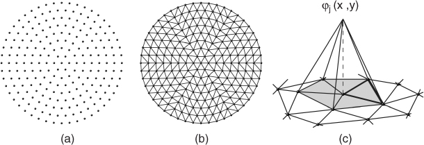
We perform triangulation of the domain Ω by subdividing Ω into triangular subdomains K1, K2, …, KM as in Figure 5.2. They are pairwise disjoint and no vertex of one triangle lies on the edge of another triangle within a typical triangular element. The corresponding approximate domain, denoted by Ωh, is the domain whose closure is the closure of K1 ∪ ··· ∪ KM.
Figure 5.2 (a) Node points, (b) finite element triangulation and (c) basis function ϕj
Next, we can construct the finite element space ![]() :
:
![]()
Let {zj:j = 1, …, N} be the set of nodes of the triangular elements. For each k, we define the function φk ∈ V by
![]()
Then, it is easy to see that
![]()
According to the Lax–Milgram theorem, there exists a unique u ∈ V that solves
Substituting ![]() (with ui being unknown constants) into (5.33) leads to the linear system
(with ui being unknown constants) into (5.33) leads to the linear system
5.34 
where
![]()
The Lax–Milgram theorem provides that the system has a unique solution u = (u1, …, uN)T satisfying

Since the rank of A is N − 1, we drop the first row and column of A and consider
5.36 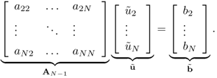
Now, AN−1 is invertible and hence we can compute ![]() . Using the knowledge of
. Using the knowledge of ![]() , we can obtain the solution u = ∑ujφj of (5.33) by
, we can obtain the solution u = ∑ujφj of (5.33) by

where c is a constant chosen so that ![]() .
.
5.5.2.1 Computation of Element Matrix
Let ![]() be the set of the triangular elements. The ijth element of the matrix A can be decomposed into
be the set of the triangular elements. The ijth element of the matrix A can be decomposed into

Fixing the triangle K, we let the nodes of K be z1, z2 and z3. Let φ1(x) be a linear function on K with the value 1 at the node z1 and 0 at the other nodes. We will derive formulas for φ1 and ∇φ1 in terms of z1, z2 and z3. The function φ1 in K can be written in the form
![]()
where α1, α2, α3 satisfy

Therefore, the coefficients α1, α2, α3 can be found from

Since we can express φ1 as

![]()
where
![]()
and ![]() is the area of the triangle. Note that φ1(x) is linear and φ1(z2) = 0 = φ1(z3).
is the area of the triangle. Note that φ1(x) is linear and φ1(z2) = 0 = φ1(z3).
Similarly, we have
![]()
![]()
Simple computation yields
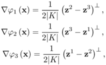
where z⊥ = (z2, − z1). If σ = σK is a constant in K, then
![]()
Hence, the element matrix for the triangular element K is

5.5.2.2 Assembly of Two Element Matrices
We can combine two element matrices from two connected triangles sharing two nodes together. Globally numbering all four nodes, we may express each element matrix as

Assembly of these two element matrices is straightforward as
![]()
5.5.2.3 Assembly of Master Matrix
We first globally number all nodes. Assembly of all element matrices into a master matrix is more complicated because we must take care of connected or disjoint elements. Since the ijth element of the matrix A is
![]()
assembly of all element matrices is required to form the global master matrix A. An efficient way of assembling the global master matrix proceeds recursively, building up the finite element representation of one element at a time, as follows.

![]()

This procedure generates a lower triangular matrix
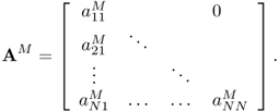
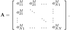
Since our master matrix A is symmetric and ![]() when i ≥ j,
when i ≥ j,
5.5.2.4 Boundary Condition
Since A is a singular matrix, it is not invertible and we cannot solve the linear system of equations Au = b. Since the rank of A is N − 1, we set a reference node and modify the master matrix so that the modified matrix is not singular, as follows.

![]()
5.5.2.5 Solution of Linear System of Equations
The matrix AN−1 is symmetric, positive definite and sparse. Hence, we can solve ![]() using various techniques introduced in the previous sections.
using various techniques introduced in the previous sections.
5.5.3 Numerical Examples
5.5.3.1 Elliptic PDE
Let Ω be a unit disk with the conductivity distribution σ given in Figure 5.3. We attach three electrodes ![]() as shown in Figure 5.3. If we apply voltage V0 between a pair of the electrodes
as shown in Figure 5.3. If we apply voltage V0 between a pair of the electrodes ![]() and
and ![]() , then the induced potential is dictated approximately by the following mixed boundary value problem:
, then the induced potential is dictated approximately by the following mixed boundary value problem:
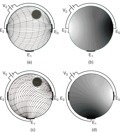
where σ is the conductivity distribution. Figure 5.4 shows the images of the current flux and equipotential lines for the solution of (5.37). The following suggests an example code for solving (5.37).
clc; clear; close all
h = 1/32; Node = [0 0];
for cir = 1:1/h
Node = [Node;cir*h*cos((0:round(2*pi*cir)-1)*2*pi/round(2*pi*cir))’
...cir*h*sin((0:round(2*pi*cir)-1)*2*pi/round(2*pi*cir))’]; end
Element = delaunayn(Node); Sol_u = zeros(length(Node),1);
Sen = zeros(length(Node)); in =length(Node)-ceil(1*round(2*pi*cir/16)):
...length(Node)-ceil(0*round(2*pi*cir/16)); Sol_u(in) = 1;
out = length(Node)-floor(9*round(2*pi*cir/16)):length(Node)-
...floor(8*round(2*pi*cir/16)); Sol_u(out) = -1;
B = [in out]; I = [];
for ele = 1:length(Element)
    Cof=[Node(Element(ele,:),:) ones(3,1)]eye(3);sigma = 1;
    if norm(mean(Node(Element(ele,:),:))-[0.5 0.5])<0.2+10^(-2)
        sigma = 2;     end
Sen(Element(ele,:),Element(ele,:)) = Sen(Element(ele,:),Element(ele,:))+sigma*
...abs(1/2*det([Node(Element(ele,:),:) ones(3,1)]))*(Cof(1:2,:)’*Cof(1:2,:));
end
Sen(B,:) = []; RHS =-Sen*Sol_u; Sen(:,B) = [];
Sol_u(setdiff(1:length(Node), find(Sol_u =0))) = SenRHS;
figure; plot(Node(:,1),Node(:,2),‘k.’); axis equal; axis off;
 hold on; plot(Node(in,1),Node(in,2),‘b*’);
hold on; plot(Node(out,1),Node(out,2),‘r*’);
hold on; plot(Node(length(Node)-ceil(9*round(2*pi*cir/16)):length(Node)
...-ceil(8*round(8*pi*cir/16)),1),Node(length(Node)-ceil(9*round(2*pi*cir/16))
...:length(Node)-ceil(8*round(8*pi*cir/16)),2),‘ms’);
figure,triplot(Element, Node(:,1), Node(:,2),‘black’); axis equal;axis off;
figure, trimesh(Element, Node(:,1), Node(:,2), Sol_u);
Figure 5.3 Conductivity distribution and mesh
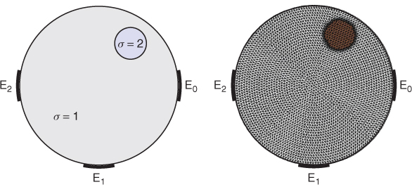
Figure 5.4 (a, c) Current flux and (b, d) equipotential lines
5.5.3.2 Poisson Equation
We consider the Poisson equation
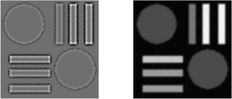
Figure 5.5 shows the image of ρ in (5.38) and the solution u. The following also suggests an example code to solve (5.38).
[X Y] = meshgrid(0:0.005:0.5,0:0.005:0.5); Node = [X(:) Y(:)];
Element = delaunayn(Node); U = ones(length (Node),1); App_U = U;
Sen = sparse(length(Node), length(Node));
U(sum((Node-ones(size(U))*[0.12 0.38])'.^{2})<0.1^{2}+0.1^{4}
…|sum((Node-ones(size(U))*[0.380.15])'.^{2})<0.1^{2}+0.1^{4}) = 4;
U((abs(Node(:,1)−0.15)<0.1+0.1^{4}&abs(Node(:,2)−0.05)<0.015+0.1^{4})
…|(abs(Node(:,1)−0.15)<0.1+0.1^{4}&abs(Node(:,2)−0.13)<0.015+0.1^{4})) = 8;
U((abs(Node(:,1)−0.15)<0.1+0.1^{4}&abs(Node(:,2)−0.2)<0.015+0.1^{4})) = 10;
U((abs(Node(:,1)−0.45)<0.015+0.1^{4}&abs(Node(:,2)−0.38)<0.1+0.1^{4})
…|(abs(Node(:,1)−0.37)<0.015+0.1^{4}&abs(Node(:,2)−0.38)<0.1+0.1^{4})) = 12;
U((abs(Node(:,1)−0.3)<0.015+0.1^{4}&abs(Node(:,2)−0.38)<0.1+0.1^{4})) = 6;
On=zeros(length(Node),10);
index=ones(length(Node),1);
for ele=1:length(Element)
    p= Element(ele,:);
    On(p(1),index(p(1)))=ele;index(p(1))=index(p(1))+1;
    On(p(2),index(p(2)))=ele;index(p(2))=index(p(2))+1;
    On(p(3),index(p(3)))=ele;index(p(3))=index(p(3))+1;
end
grad_u=gradp(Node,Element,U);grad=ele2node(On,grad_u);clear grad_u;
…grad_ux=gradp(Node,Element,grad(:,1));gradx=ele2node(On,grad_ux);
grad_uy=gradp(Node,Element, grad(:,2)); grady=ele2node(On,grad_uy);
f=−(gradx(:,1) + grady(:,2));RHS=zeros(size(U)); figure;
surfc(X,Y,reshape(f,size(X,1),size(X,2)),‘FaceColor’,‘interp’,
…‘EdgeColor’,‘none’);view(2);colormap gray; axis equal; axis off;
for ele = 1:length(Element)
Cof = [Node(Element(ele,:),:) ones(3,1)]eye(3);
Sen(Element(ele,:),Element(ele,:)) = Sen(Element(ele,:),Element(ele,:))+abs
…(1/2*det([Node(Element(ele,:),:) ones(3,1)]))*(Cof(1:2,:)'*Cof(1:2,:));
RHS(Element(ele,:)) = RHS(Element(ele,:))+f(Element(ele,:))
…*abs(1/factorial(2)*det([Node(Element(ele,:),:) ones(3,1)]))/3;
end
B = find((Node(:,1)−0.25)>0.246 & (Node(:,2)−0.25)>0.246); clear Node
Sen(B,:) = [];RHS(B) = [];RHS=RHS-Sen*App_U; Sen(:,B) = [];
App_U(setdiff(1:length(X(:)),B)) = SenRHS;
figure;surfc(X,Y,reshape(App_U,size(X,1),size(X,2)),‘FaceColor’,
…‘interp’,‘EdgeColor’,‘none’);view(2); colormap gray; axis equal; axis off;
function grad_u=gradp(Node,ele_con,fwd_potential)
%%%how to get gradient potential~~~
num=length(ele_con);
for ele = 1:num
         vertex=ele_con(ele,:);%%%four vertex of tetrahedron
         Jacobian(1,:) = Node(vertex(1),:)-Node(vertex(3),:);
         Jacobian(2,:) = Node(vertex(2),:)-Node(vertex(3),:);
         %%%%Jacobian is the Jacobian Matrix
         %%%%pd=potential difference
         PD(1)=fwd_potential(vertex(1))-fwd_potential(vertex(3));
         PD(2)=fwd_potential(vertex(2))-fwd_potential(vertex(3));
         grad_u(ele,:) = JacobianPD';
end
function grad=ele2node(On,gradp)
%%  this function is just for 2D,
% transfer the gradient in each element to gradient in each Node
grad=zeros(size(On,1),2);
for i=1:size(On,1)
    if length(find(On(i,:)>0))==1
       grad(i,:)=gradp(On(i,find(On(i,:)>0)),:);
    else
    grad(i,:)=mean(gradp(On(i,find(On(i,:)>0)),:));
    end
end
Figure 5.5 Image of ρ and solution of the Poisson equation in (5.38)
References
Allen MB, Herrera I and Pinder GF 1988 Numerical Modeling in Science and Engineering. John Wiley & Sons, Inc., New York.
Haberman R 1987 Elementary Applied PDEs, 2nd edn. Prentice-Hall, Englewood Cliffs, NJ.
Johnson C 2009 Numerical Solution of Partial Differential Equations by the Finite Element Method. Reprint of 1987 edition. Dover, Mineola, NY.
Lax PD and Richtmyer RD 1956 Survey of the stability of linear finite difference equations. Commun. Pure Appl. Math. 9, 267–293.
Further Reading
Axelsson O and Barker VA 1984 Finite Element Solution of Boundary Value Problems: Theory and Computation. Academic Press, Orlando, FL.
Bank RE 1998 PLTMG: A Software Package for Solving Elliptic Partial Differential Equations. Users' Guide 8.0. Software, Environments, Tools, vol. 5. SIAM, Philadelphia, PA.
Braess D 2007 Finite Elements: Theory, Fast Solvers, and Applications in Elasticity Theory, 3rd edn. Translated from German by LL Schumaker. Cambridge University Press, Cambridge.
Brenner SC and Scott LR 2008 The Mathematical Theory of Finite Element Methods, 3rd edn. Texts in Applied Mathematics, vol. 15. Springer, New York.
Brezzi F and Fortin M 1991 Mixed and Hybrid Finite Element Methods. Springer Series in Computational Mathematics, vol. 15. Springer, New York.
Brezzi F, Marini LD, Markowich P and Pietra P 1991 On some numerical problems in semiconductor device simulation. In Mathematical Aspects of Fluid and Plasma Dynamics (eds G Toscani, V Boffi and S Rionero). Lecture Notes in Mathematics, vol. 1460, pp. 31–42. Springer, Berlin.
Calhoun D and LeVeque RJ 2005 An accuracy study of mesh refinement on mapped grids. In Adaptive Mesh Refinement—Theory and Applications. Lecture Notes in Computer Science and Engineering, no. 41, pp. 91–101. Springer, Berlin.
Carstensen C and Klose R 2003 A posteriori finite element error control for the p-Laplace problem. SIAM J. Sci. Comput. 25(3), 792–814.
Carstensen C, Liu W and Yan N 2006 A posteriori error estimates for finite element approximation of parabolic p-Laplacian. SIAM J. Numer. Anal. 43(6), 2294–2319.
Ciarlet PG 1980 Metod Konechnykh Elementov dlya Ellipticheskikh Zadach. Translated from English by BI Kvasov. Mir, Moscow.
Fehrenbach J, Gournay F, Pierre C and Plouraboue F 2012 The generalized Graetz problem in finite domains. SIAM J. Appl. Math. 72(1), 99–123.
Gockenbach MS 2006 Understanding and Implementing the Finite Element Method. SIAM, Philadelphia, PA.
Higham DJ and Higham NJ 2005 MATLAB Guide, 2nd edn. SIAM, Philadelphia, PA.
Iserles A 1996 A First Course in the Numerical Analysis of Differential Equations. Cambridge Texts in Applied Mathematics. Cambridge University Press, Cambridge.
LeVeque RJ 2002 Finite Volume Methods for Hyperbolic Problems. Cambridge Texts in Applied Mathematics. Cambridge University Press, Cambridge.
LeVeque RJ 2007 Finite Difference Methods for Ordinary and Partial Differential Equations: Steady-State and Time-Dependent Problems. SIAM, Philadelphia, PA.
Moler CB 2004 Numerical Computing with MATLAB. SIAM, Philadelphia, PA.
Quarteroni A and Valli A 1994 Numerical Approximation of Partial Differential Equations. Springer Series in Computational Mathematics, vol. 23. Springer, Berlin.
Quarteroni A and Saleri F 2003 Scientific Computing with MATLAB. Texts in Computational Science and Engineering, vol. 2. Springer, Berlin.
Richtmyer RD and Morton KW 1967 Difference Methods for Initial-Value Problems, 2nd edn. Interscience Tracts in Pure and Applied Mathematics, no. 4. Interscience, New York.
Strang G and Fix G 2008 An Analysis of the Finite Element Method, 2nd edn. Wellesley-Cambridge, Wellesley, MA.
Strikwerda JC 1989 Finite Difference Schemes and Partial Differential Equations. Wadsworth & Brooks/Cole Mathematics Series. Wadsworth & Brooks/Cole, Pacific Grove, CA.
Thomas JW 1995 Numerical Partial Differential Equations: Finite Difference Methods. Texts in Applied Mathematics, vol. 22. Springer, New York.
Trefethen LN Spectral Methods in MATLAB Software, Environments, Tools, vol. 10. SIAM, Philadelphia, PA.


