Chapter 6
CT, MRI and Image Processing Problems
Image processing has become one of the most important components in medical imaging modalities such as magnetic resonance imaging, computed tomography, ultrasound and other functional imaging modalities. Image processing techniques such as image restoration and sparse sensing are being used to deal with various imperfections in the data acquisition processes of the imaging modalities. Image segmentation, referring to the process of partitioning an image into multiple segments, has numerous applications, including tumor detection, quantification of tissue volume, computer-guided surgery, study of anatomical structure and so on. In this chapter, we review the basic mathematics behind X-ray computed tomography (CT) and magnetic resonance imaging (MRI), and then discuss some image processing techniques.
6.1 X-ray Computed Tomography
X-ray computed tomography (CT) is the most widely used tomographic imaging technique, which uses X-rays passing through the body at different angles. It visualizes the internal structures of the human body by assigning an X-ray attenuation coefficient to each pixel, which characterizes how easily a medium can be penetrated by an X-ray beam Hounsfield (1973). The idea is to visualize the imaging object in a slice by taking X-ray data at all angles around the object based on mathematical methods suggested by Cormack (1963). They shared the 1979 Nobel Prize. Indeed, some of the ideas of CT (reconstructing cross-sectional images of an object from its integral values along lines in all directions) were previously developed by Radon (1917). Bracewell (1956) had applied his theory to radioastronomy, but unfortunately little attention was paid to it at that time. Cormack was unaware of Radon's earlier work, and Radon himself did not know the even earlier work by the Dutch physicist Lorentz, who had already proposed a solution of the mathematical problem for the three-dimensional case (Cormack 1992). We refer to Kalender (2006) for an excellent review of CT.
6.1.1 Inverse Problem
The corresponding inverse problem to X-ray CT can be described roughly as follows.
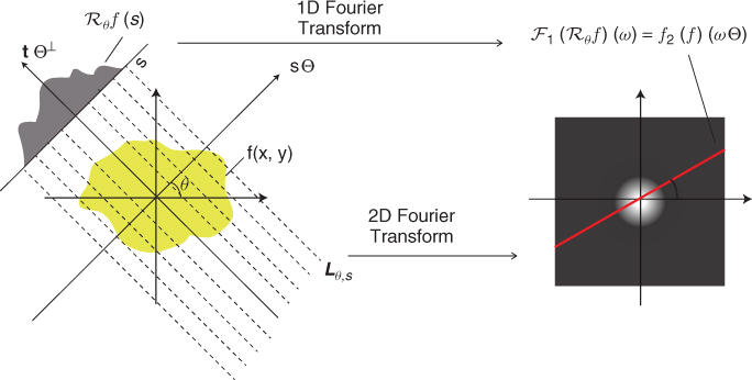
- Quantity to be imaged. The distribution of linear attenuation coefficients, denoted by a function f(x) at point x = (x1, x2) or x = (x1, x2, x3). See Figure 6.1.
- Input data. An incident X-ray beam is passed through a patient placed between an X-ray source and a detector. These beams are transmitted in all directions Θ: = (cosθ, sinθ), 0 ≤ θ ≤ 2π. Assuming a fixed angle θ, a number of X-ray photons are transmitted through the body along projection lines
 ,
,  . See Figure 6.1.
 - Output data. Detectors measure X-ray intensity attenuation Iθ(s) along the individual projection lines Lθ, s at all angles. These measured data Iθ(s) provide an X-ray image Pθ(s) that can be expressed roughly by
- Inverse problem. Recover f from the series of X-ray data
 , where θn = 2nπ/N.
Figure 6.1 Illustration of the Fourier slice theorem
6.1.2 Basic Principle and Nonlinear Effects
We begin with understanding the relationship between X-ray intensity attenuation Iθ(s) and the X-ray data Pθ(s) in (6.1). For simplicity, we ignore scattering and metal shadowing effects for the moment.
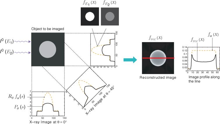
Fix θ and s. The incident X-ray beam is composed of a number of photons of different energies. Hence, the incident intensity of the X-ray beam, denoted by I0, can be viewed as a function of the photon energy level E (Brooks and Chiro 1976). Imagine that an X-ray passes through a patient along Lθ, s. Let Iθ(E, s) be the measured attenuated intensity along the line Lθ, s. Then I0(E) indicates the source X-ray at energy level E, and Iθ(E, s) indicates the detected X-ray after passing through the body along the line Lθ, s. Denoting by fE(x) the attenuation coefficient at point x and at energy level E, the relation between Iθ(E, s) and fE is dictated by the Beer–Lambert law (Beer 1852; Lambert 1760):
6.3 ![]()
where Emax and Emin, respectively, are the maximum and minimum energy levels of the X-ray beam. Soft tissues have roughly fE = 0.38 at E = 30 keV cm−1 and fE = 0.21 at E = 60 keV cm−1. If the beam does not interact with any medium, then the unattenuated beam is Iθ(E, s) = I0(E).
![]()
Figure 6.2 Illustration of metal artifacts
The measured attenuation intensity Iθ(s) along the projection line Lθ, s is given by
6.4 ![]()
This Iθ(s) provides the X-ray data Pθ(s) given by
6.5 ![]()
We try to reconstruct an image f such that
6.6 ![]()
We hope that f is related to ![]() for some energy level E0.
for some energy level E0.
6.7 ![]()
6.8 ![]()
6.10 
6.1.3 Inverse Radon Transform
Recall that the Radon transform ![]() of an attenuation coefficient f(x) is the one-dimensional projection of f(x) taken at an angle θ. Let
of an attenuation coefficient f(x) is the one-dimensional projection of f(x) taken at an angle θ. Let ![]() denote the projection map in (6.2) as a function of θ and s, which can be expressed as
denote the projection map in (6.2) as a function of θ and s, which can be expressed as
6.12 ![]()
The back-projection operator associated with the projection map ![]() is defined by
is defined by
6.13 ![]()
The Hilbert transform of a function ϕ(t) is defined as
6.14 ![]()
6.15 ![]()
![]()
6.16 ![]()
In order to prove this theorem, we need to know the following Fourier slice theorem.
6.18 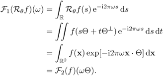
Now, we are ready to prove the inverse Radon transform.
![]()
can be changed into the polar coordinate form
![]()
Using (6.17), we can change the form again into the following:
Denoting ![]() , we obtain
, we obtain
because
![]()
Hence, it follows from (6.19) and (6.20)) that
6.21 
This completes the proof of the inverse Radon transform.
6.22 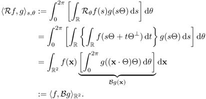
![]()
![]()
![]()
![]()
6.23 ![]()
We refer to Faridani (2003) and Natterer (2008) for detailed explanations on the Radon inversion formula, and refer to Tuy (1983), Feldkamp et al. (1984), Kak and Slaney (1988) and Grangeat (1991) for the inversion algorithm in cone-beam CT, which uses a cone-shaped X-ray beam rather than a conventional linear fan beam.
6.1.4 Artifacts in CT
In X-ray CT, the incident intensity I0(E) and the attenuated intensity Iθ(E, s) are functions of the energy level E, which ranges over 10–150 keV, and the attenuation coefficient fE differs with the energy level E. Mostly, ∂fE/∂E < 0, which means that the lower-energy photons are absorbed more rapidly than higher-energy photons. Hence, there exist fundamental artifacts in the reconstructed image f(x) as in Figure 6.2 by the inverse Radon transform since f can be regarded as a distribution of the linear attenuation coefficient f(x) ≈ f(x) at a mean energy level E0.
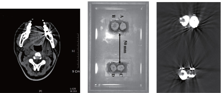
The presence of metal objects in the scan field can lead to severe streaking artifacts owing to the above-mentioned inconsistencies by beam hardening and severely high contrast in the attenuation coefficient distribution between the metal and the surrounding subjects. Figure 6.3 shows such metal artifacts. Additional artifacts due to beam hardening, partial volume and aliasing are likely to compound the problem when scanning very dense objects. We refer to Kalender et al. (1987), Meyer et al. (2010) and Wang et al. (1996) for metal artifacts reduction.
![]()
Figure 6.3 Examples of metal artifacts
6.2 Magnetic Resonance Imaging
MRI uses magnetic fields to visualize the quantity of hydrogen atoms inside biological tissues by creating magnetization; hydrogen atoms can interact with the external magnetic field B because a nucleus with spin has a local magnetic field around it. In the human body, the amount of hydrogen would be the major factor of the net magnetization vector M. In MRI, we use various techniques to localize M in such a way that we provide a cross-sectional image of the density of M inside the human body. These techniques are based on the nuclear magnetic resonance (NMR) phenomenon, which is determined by the interaction of a nuclear spin M with the external magnetic field B and its local environments, including relaxation effects.
The idea behind this imaging modality was published by Lauterbur (1973), and the first cross-sectional image of a living mouse was published by Lauterbur (1974). Damadian (1971) discovered that NMR can distinguish tumors from normal tissues due to their relaxation time. Lauterbur and Mansfield were awarded the Nobel Prize for developing the mathematical framework and some MRI techniques, but the award was denied by Damadian, who claimed that his work was earlier than those of Lauterbur and Mansfield. We refer to Filler (2010) for the history of MRI. We will describe the NMR phenomenon in the next section, taking account of measurable signals in an MRI system.
6.2.1 Basic Principle
We consider a human body occupying a domain Ω inside an MRI scanner with its main magnetic field B0 + δB. Throughout this section, we shall assume that the field inhomogeneity δB is negligible, that is, δB = 0 and ![]() is constant. The strong uniform main field produces a distribution of net magnetization M(r, t) in Ω by aligning protons inside the human body, where
is constant. The strong uniform main field produces a distribution of net magnetization M(r, t) in Ω by aligning protons inside the human body, where ![]() depends on time t and position r. A stronger B0 produces a larger
depends on time t and position r. A stronger B0 produces a larger ![]() . The interaction of
. The interaction of ![]() with the external magnetic field B0 is dictated by the Bloch equation:
with the external magnetic field B0 is dictated by the Bloch equation:
where γ is the gyromagnetic ratio1. From (6.24), we have
6.25 ![]()
which means that the vector ∂M/∂t is perpendicular to both M and B0. To be precise, (6.24) can be written as
6.26 
Writing M⊥ = Mx + iMy, we express the above identity as
6.27 ![]()
The solution of the above ODE is
which means that the transverse component M⊥ rotates clockwise at the angular frequency ![]() . The above expression explains how B0 causes M to precess around the z axis at the angular frequency of
. The above expression explains how B0 causes M to precess around the z axis at the angular frequency of ![]() . For a 1.5 T MRI system, the frequency of
. For a 1.5 T MRI system, the frequency of ![]() is approximately 64 MHz. According to (6.28),
is approximately 64 MHz. According to (6.28), ![]() causes M to precess clockwise about the
causes M to precess clockwise about the ![]() direction at the angular frequency
direction at the angular frequency ![]() . If we apply a magnetic field B(r), then M(r, t) satisfies the Bloch equation
. If we apply a magnetic field B(r), then M(r, t) satisfies the Bloch equation
![]()
and M(r, t) precesses at the angular frequency ![]() .
.
6.2.2 k-Space Data
If we could produce a magnetic flux density B that is localized at each position r (in such a way that ![]() ), we could encode the positions independently. However, it is impossible to localize the magnetic field B because ∇ · B = 0. Instead of a point localization, we could make a slice localization by applying a magnetic field gradient that varies with respect to one direction. The following is the one-dimensional magnetic field gradient along the z axis with the magnetic field increasing in the z direction:
), we could encode the positions independently. However, it is impossible to localize the magnetic field B because ∇ · B = 0. Instead of a point localization, we could make a slice localization by applying a magnetic field gradient that varies with respect to one direction. The following is the one-dimensional magnetic field gradient along the z axis with the magnetic field increasing in the z direction:
6.29 ![]()
where B0 and Gz are constants. The first component B0 is the main magnetic field, which causes individual M(r) to precess around the z axis, and the second term ![]() is the gradient field. This Gz is said to be the magnetic field gradient in the z direction. With this B, the vector M in the body is essentially vertically aligned and rotates at the Larmor frequency γ(B0 + Gzz) around the z axis. Note that the frequency changes with z.
is the gradient field. This Gz is said to be the magnetic field gradient in the z direction. With this B, the vector M in the body is essentially vertically aligned and rotates at the Larmor frequency γ(B0 + Gzz) around the z axis. Note that the frequency changes with z.
To extract a signal of M, we flip M toward the transverse direction to produce its xy component. Flipping M toward the xy plane requires a second magnetic field B1 perpendicular to B0 = (0, 0, B0). We can flip M over the xy plane by using a radio-frequency (RF) magnetic field B1 that is generated by RF coils through which we inject sinusoidal current at the Larmor frequency ![]() .
.
After terminating the RF pulse, we apply a phase encoding gradient in the y direction, which makes the spin phase change linearly in the phase encoding direction. Then we apply the frequency encoding gradient field as
![]()
and the signal during frequency encoding in the x direction becomes
Through multiple phase encodings to get multiple signals of (6.30) for different values of ky, we may collect a set of k-space data
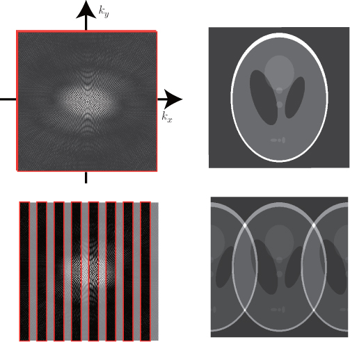
for various kx and ky. See Figure 6.4 (top left) for an image of S(kx, ky). We refer the reader to the book by Haacke et al. (1999) for detailed explanations on MRI.
Figure 6.4 The two images at the top are fully sampled k-space data and the inverse Fourier transform. The two images at the bottom are subsampled k-space data by the factor of 2 and the inverse Fourier transform
6.2.3 Image Reconstruction
In the Cartesian sampling pattern, we select a cross-sectional slice in the z direction using the gradient coils and get spatial information in the xy plane using the frequency encoding (x direction) and phase encoding (y direction). Let m be a spin density supported in the region {(x, y): − FOV/2 < x, y < FOV/2}, where FOV is the field of view, and let m be the N2 column vector representing the corresponding N × N image matrix with pixel size Δx × Δy = FOV/N × FOV/N. The inverse Fourier transform provides the image of m(x, y) (see Figure 6.4 (top right)). Let us quickly review the inverse discrete Fourier transform (DFT). Assume that the image of m(x, y) is approximated by an N × N matrix m:

Then, the relation (6.26) between the MR data and the image of m(x, y) can be expressed as
6.32 
for some scaling constant c and j, ![]() = 0, 1, …, N − 1. Here, the inverse DFT with a k-space sampling that is designed to meet the Nyquist criterion provides a discrete version of the image m(x, y). Using the two-dimensional inverse DFT, we have
= 0, 1, …, N − 1. Here, the inverse DFT with a k-space sampling that is designed to meet the Nyquist criterion provides a discrete version of the image m(x, y). Using the two-dimensional inverse DFT, we have
6.33 
for some scaling constant ![]() .
.
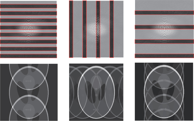
In MRI, the data acquisition speed is roughly proportional to the number of phase encoding lines due to the time-consuming phase encoding, which separates signals from different y positions within the image m(x, y). Hence, to accelerate the acquisition process, we need to skip phase encoding lines in k-space. Definitely, reduction in the k-space data violating the Nyquist criterion is associated with aliasing in the image space. If we use subsampled k-space data by a factor of R in the phase encoding direction (y direction), according to the Poisson summation formula, the corresponding inverse Fourier transform produces the following fold-over artifacts (as shown in Figure 6.4 (bottom right) and Figure 6.5):

Figure 6.5 The images at the top are subsampled k-space data sets. The images at the bottom are the corresponding inverse Fourier transforms
Parallel MRI (pMRI) is a way to deal with this fold-over artifact by using multiple receiver coils and supplementary spatial information in the image space. Parallel imaging has received a great deal of attention since the work by Sodickson and Manning (1997), Sodickson et al. (1999) and Pruessmann et al. (1999). In pMRI, we skip phase encoding lines in k-space during MRI acquisitions in order to reduce the time-consuming phase encoding steps, and in the image reconstruction step, we compensate the skipped k-space data by the use of space-dependent properties of multiple receiver coils. Numerous parallel reconstruction algorithms such as SENSE, SMASH and GRAPPA have been suggested, and those aim to use the least possible data of phase encoding lines, while eliminating aliasing, which is a consequence of violating the Nyquist criterion by skipping the data. We refer to Jakob et al. (1998), Kyriakos et al. (2000), Heidemann et al. (2001), Pruessmann et al. (2001), Bydder et al. (2002) and Griswold et al. (2002) for pMRI algorithms and to Larkman and Nunes (2001) for a review.
6.3 Image Restoration
Numerous algorithms for image restoration and segmentation are based on mathematical models with partial differential equations, level set methods, regularization, energy functionals and others. In these models, we regard the intensity image as a two-dimensional surface in a three-dimensional space with the gray level assigned to the axis. We can use the distribution of its gradient, Laplacian and curvature to interpret the image. For example, Canny (1986) defined edge points as points where the gradient magnitude assumes a local maximum in the gradient direction. The noise is usually characterized as having a local high curvature. Using these properties, one may decompose the image roughly into features, background, texture and noise. Image processing techniques are useful tools for improving the detectability of diagnostic features. We refer the reader to the books by Aubert and Kornprobst (2002) and Osher et al. (2002) for PDE-based image processing.
For clear and easy explanation, we restrict ourselves to the case of a two-dimensional grayscale image that is expressed as a function u ∈ L2(Ω) in the rectangular domain Ω = {x = (x, y):0 < x, y < 1}. Throughout this section, we assume that the measured (or observed) image f ∈ L2(Ω) and the true image u are related by
6.34 ![]()
where η represents noise and H is a linear operator including blurring and shifting. For image restoration and segmentation, we use a priori knowledge about the geometric structure of the surface {(x, u(x)):x ∈ Ω} in the three-dimensional space.
The goal of denoising is to filter out noise while preserving important features. If the noise η is Gaussian random noise satisfying ∫η = 0, we can apply the Gaussian kernel
![]()
to get an approximation
![]()
with an appropriate choice of variance σ > 0. Note that Gt * f(x) is a solution of the heat equation with the initial data f(x):

Hence, we expect that this smoothing method eliminates highly oscillatory noise that results in Gσ * (Hu + η) ≈ Gσ * (Hu), while edges having high frequencies are also smeared at the same time. Several schemes have been proposed to deal with this blurring problem.
A typical way of denoising (or image restoration) is to find the best function by minimizing the functional:
where the first term ![]() , called the fidelity term, forces the residual Hu − f to be small, the second term
, called the fidelity term, forces the residual Hu − f to be small, the second term ![]() , called the regularization term, enforces the regularity of u, and λ, called the regularization parameter, controls the tradeoff between the residual norm and the regularity. We can associate (6.35) with the Euler–Lagrange equation:
, called the regularization term, enforces the regularity of u, and λ, called the regularization parameter, controls the tradeoff between the residual norm and the regularity. We can associate (6.35) with the Euler–Lagrange equation:
6.36 ![]()
where H* is the dual of H. The above equation is nonlinear except for p = 2. When p = 2, the minimizer u satisfies the linear PDE,
![]()
which has computational advantages in computing u. But the Laplace operator has very strong isotropic smoothing properties and does not preserve edges because it penalizes the strong gradients along edges. This is the major reason why many researchers use p = 1 since it does not penalize the gradients along edges with alleviating noise:
![]()
We can solve (6.35) using the gradient descent method by introducing the time variable t:
6.37 ![]()
To understand the above derivation, we present the following simple example.
![]()
![]()
![]()
![]()
![]()
![]()
6.3.1 Role of p in (6.35)
Let us investigate the role of the diffusion term ∇(|∇u|p−2∇u) in (6.35). The image u(x) can be viewed as a two-dimensional surface {(r, u(r)):(x, y) ∈ Ω}. To understand the image structure, we look at the level curve ![]() , the curve along which the intensity u(x) is a constant c. Let x(s) represent a parameterization of the level curve
, the curve along which the intensity u(x) is a constant c. Let x(s) represent a parameterization of the level curve ![]() , that is,
, that is, ![]() . The normal vector and tangent vector to the level curve
. The normal vector and tangent vector to the level curve ![]() , respectively, are
, respectively, are
![]()
where ux = ∂u/∂x and uy = ∂u/∂y. Let us investigate the double derivative of u in the tangent and normal directions:
![]()
where (D2u) is the Hessian matrix of u. Direct computation shows that

This leads to
![]()
Substituting ux = − y′|∇u|/|x′| and uy = x′|∇u|/|x′| into the above identity and with 0 = ∇u · x′, we obtain

where ∇ · n = κ is the curvature. Hence,
Similarly, we have
- In the case p = 2, we have the following isotropic diffusion:
![]()
6.41 ![]()
The diffusion rate in the T direction is |∇u|p−2, while the diffusion rate in the n direction is (p − 1)|∇u|p−2. Since n is normal to the edges, it would be preferable to smooth more in the tangential direction than in the normal direction. In order to preserve edges, p = 1 would be best, since it annihilates the coefficient of unn.
6.3.2 Total Variation Restoration
In one dimension, the total variation (TV) of a signal f defined in an interval [0, 1] means the total amplitude of signal oscillations in [0, 1]. The classical definition of the total variation of f is
where the supremum is taken over all partitions in the interval [0, 1]. The space of bounded variation functions in [0, 1], denoted by BV([0, 1]), is the space of all real-valued functions f ∈ L1([0, 1]) such that ||f||BV([0, 1]) < ∞. In the special case when f ∈ C1([0, 1]) is differentiable, it can be defined by
The classical definition (6.42) of BV in one dimension is not suitable in the two- or three-dimensional cases. Hence, we use the following definition that is closely related to (6.43):
6.44 
Now, we come back to the two-dimensional grayscale image u(r) defined in the rectangular domain Ω = {r = (x, y):0 < x, y < 1}.
6.45 ![]()
6.46 ![]()
![]()
![]()
![]()
![]()
![]()
![]()
![]()
For a smooth domain D, the bounded variation of the characteristic function χD is
![]()
In general, according to the co-area formula, the total variation of ![]() can be expressed as
can be expressed as
![]()
Now, we are ready to explain the TV restoration that is the case for p = 1 in (6.35):
6.47 ![]()
Assuming that H is a linear operator with its dual H*, this is associated with the nonlinear Euler–Lagrange equation:
Hence, the minimizer u can be obtained from the standard method of solving the corresponding time marching algorithm:
6.49 
To understand TV denoising effects, consider a smooth function u satisfying
For a fixed value ![]() , let
, let ![]() be a simply closed curve in Ω such that u(x, t) = α on
be a simply closed curve in Ω such that u(x, t) = α on ![]() and u(x, t) > α inside
and u(x, t) > α inside ![]() . Since u satisfies the nonlinear diffusion equation (6.50),
. Since u satisfies the nonlinear diffusion equation (6.50),
![]()
Note that the outer normal vector n on ![]() can be represented as
can be represented as
![]()
where ![]() denotes the sign of u(x, t) − α in
denotes the sign of u(x, t) − α in ![]() . Hence, we have
. Hence, we have
6.51 ![]()
and therefore
![]()
or
![]()
Hence, the TV regularization quickly removes smaller-scale noise where the level set ratio ![]() is very large.
is very large.
According to (6.48), the noisy image f can be decomposed into
6.52 ![]()
where u is a minimizer of the TV-based ROF (Rudin–Osher–Fatemi) model (Rudin et al 1992)
![]()
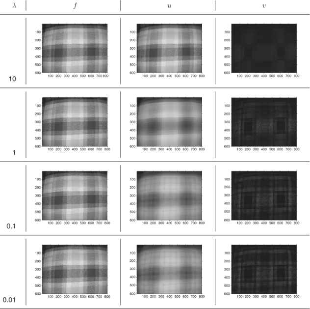
With the use of the G-norm introduced by Meyer (2002), we can understand the role of the parameter λ more precisely (see Figure 6.6):
 and v = f, where
  is the G-norm of v given by
![]()
![]()
 and
and 
The G-space is somehow very close to the dual of the BV space because of the following inequality:
![]()
![]()

![]()
![]()
![]()
Figure 6.6 Role of the parameter λ: f is the noisy image; u is the image reconstructed by the TV-based ROF model; and v = f − u
6.3.3 Anisotropic Edge-Preserving Diffusion
Diffusion PDE can act as a smoothing tool for removing high-frequency noise in the surface {(x, u(x)):x ∈ Ω}. In the previous section, we learnt that the TV restoration performs an anisotropic diffusion process by smoothing the surface except cliffs and preventing diffusion across cliffs. This type of edge-preserving diffusion technique has been widely used in the image processing community after Perona and Malik (1990) proposed an anisotropic diffusion model.
We begin by studying the general Perona–Malik model:
where ut = ∂u/∂t. This is a nonlinear PDE expressing the fact that the time change of u is equal to the negative of the divergence of the current − P(|∇u|2)∇u. It follows from (6.38) and (6.39) that

where Q(|∇v|2) = P(|∇v|2) + 2|∇v|2P′(|∇v|2), n(x) = ∇u/|∇u| and T = ( − uy, ux)/ |∇u|. Hence, the Perona–Malik model in (6.53) can be expressed as
6.54 ![]()
From the standard arguments about diffusion equations, we conclude the following:
- Q(|∇u|) > 0
 forward diffusion along ∇u direction
  edge blurring.
 - Q(|∇u|) < 0
 backward diffusion along ∇u direction
  edge sharpening.
Based on this observation, Perona and Malik (1990) proposed the diffusion coefficient
![]()
which corresponds to the concave energy functional
![]()
Note that the corresponding Perona–Malik PDE (forward–backward diffusion equation) has the following property:
- |∇u| < K
 forward diffusion along ∇u direction
  blurring.
 - |∇u| > K
 backward diffusion along ∇u direction
  edge sharpening.
Hence, the Perona–Malik PDE permits forward diffusion along the edges while sharpening across the edge (Perona and Malik 1990). However, this Perona–Malik PDE raises issues on the discrepancy between numerical and theoretical results in that it is formally ill-posed in the sense of Hadamard, whereas its discrete PDE is nevertheless numerically found to be stable by Calder and Mansouri (2011). Kichenassamy (1997) investigated this phenomenon, termed the Perona–Malik paradox, in which the Perona–Malik PDE admits stable schemes for the initial value problem without a weak solution.
![]()
6.3.4 Sparse Sensing
Fast imaging in MRI by accelerating the acquisition is a very important issue since it has a wide range of clinical applications such as cardiac MRI, functional MRI (fMRI), MRE, MREIT and so on. To reduce the MR data acquisition time, we need to skip as many phase encoding lines as possible (violating the Nyquist criterion) in k-space during MRI data acquisitions to minimize the time-consuming phase encoding step. In this case, we need to deal with the under-determined linear problem such as
We know that this under-determined linear system (6.55) has an infinite number of solutions since the null space has dim(N(A)) ≥ N − m. Without having some knowledge about the true solution, such as sparsity (having a few non-zero entries of the solution), there is no hope of solving the under-determined linear system (6.55).
Imagine that the true solution, denoted by xtrue, has sparsity. Is it possible to reconstruct xtrue by enforcing the sparsity constraint in the under-determined linear system in (6.55)? If so, can the solution be computed reliably? Surprisingly, this very basic linear algebra problem was not studied in depth until 1990.
Donoho and Elad (2003) found the following uniqueness result by introducing the concept of the spark of A:

where ![]() indicates the number of non-zero entries of x.
indicates the number of non-zero entries of x.
![]()
![]()
For S = 1, 2, 3, …, define the set
![]()
Although the under-determined linear system (6.55) has infinitely many solutions in ![]() , according to Theorem 6.3.8, it has at most one solution within the restricted set WS for
, according to Theorem 6.3.8, it has at most one solution within the restricted set WS for ![]() . Hence, one may consider the following sparse optimization problem:
. Hence, one may consider the following sparse optimization problem:
6.56 ![]()
Let x0 be a solution of the ![]() 0-minimization problem (P0). Unfortunately, finding x0 via
0-minimization problem (P0). Unfortunately, finding x0 via ![]() 0-minimization is extremely difficult (NP-hard) due to lack of convexity; we cannot use Newton's iteration.
0-minimization is extremely difficult (NP-hard) due to lack of convexity; we cannot use Newton's iteration.
Admitting fundamental difficulties in handling the ![]() 0-minimization problem (P0), it would be desirable to find a feasible approach for solving the problem (P0). One can consider the relaxed
0-minimization problem (P0), it would be desirable to find a feasible approach for solving the problem (P0). One can consider the relaxed ![]() 1-minimization problem that is the closest convex minimization problem to (P0):
1-minimization problem that is the closest convex minimization problem to (P0):
6.57 ![]()
Let x1 be a solution of the ![]() 1-minimization problem (P1). Then, can the sparsest solution of (P0) be the solution of (P1)? If yes, when? Donoho and Elad (2003) observed that it could be x0 = x1 when ||x0||0 is sufficiently small and A has incoherent columns. Here, the mutual coherence of A measures the largest correlation between different columns from A. For more details see Donoho and Huo (1999).
1-minimization problem (P1). Then, can the sparsest solution of (P0) be the solution of (P1)? If yes, when? Donoho and Elad (2003) observed that it could be x0 = x1 when ||x0||0 is sufficiently small and A has incoherent columns. Here, the mutual coherence of A measures the largest correlation between different columns from A. For more details see Donoho and Huo (1999).
For robustness of compressed sensing, Candès and Tao (2005) used the notion of the restricted isometry property (RIP) condition: A is said to have RIP of order S if there exists an isometry constant δS ∈ (0, 1) such that
6.58 ![]()
If A has RIP of order 2S, then the under-determined linear system (6.55) is well-distinguishable within the S-sparse set WS:
![]()
If δ2S < 1, then the map A is injective within the set WS. If δ2S is close to 0, the transformation A roughly preserves the distance between any two different points.
Candès et al. (2006b) observed that the sparse solution of the problem (P0) can be found by solving (P1) under the assumption that A obeys the 2S-restricted isometry property (RIP) condition with δ2S being not close to one (Candès and Tao 2005; Candès et al. 2006a).
![]()
![]()
![]()

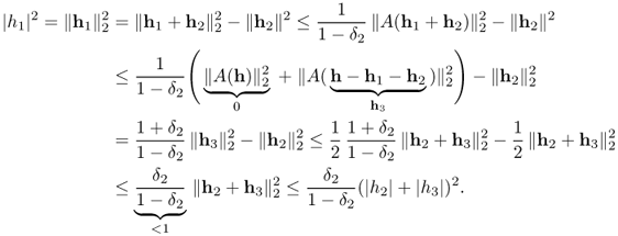
From the above theorem, if the true solution xexact is S-sparse, then x1 = xexact = x0, where x0 is a solution of (P0). Theorem 6.3.10 also provides robustness of compressed sensing. Consider the case where the measurements b are corrupted by bounded noise in such a way that
![]()
6.61 ![]()
![]()
Lustig et al. (2007) applied these sparse sensing techniques for fast MR imaging. They demonstrated high acceleration in in vivo experiments and showed that the sparsity of MR images can be exploited to reduce scan time significantly, or alternatively to improve the resolution of MR images.
6.4 Segmentation
Image segmentation of a target object in the form of a closed curve has numerous medical applications, such as anomaly detection, quantification of tissue volume, planning of surgical interventions, motion tracking for functional imaging and others. With advances in medical imaging technologies, many innovative methods of performing segmentation have been proposed over the past few decades, and these segmentation techniques are based on the basic recipes using thresholding and edge-based detection. In this section, we only consider edge-based methods, which use the strength of the image gradient along the boundary between the target object and the background.
6.4.1 Active Contour Method
The most commonly used method of segmentation in the form of a closed curve would be (explicit or implicit) active contour methods that use an application-dependent energy functional to evolve an active contour toward the boundary of the target region; the direction of the velocity of the active contour is the negative direction of the gradient of the energy functional.
To be precise, let u be a given image. We begin by considering the minimization problem of finding a closed curve ![]() that minimizes the energy functional
that minimizes the energy functional
6.62 ![]()
where g(α) is a decreasing function, for example, g(α) = 1/(1 + α). For computation of a local minimum ![]() of the functional, we may start from an initial contour
of the functional, we may start from an initial contour ![]() and consider a sequence
and consider a sequence ![]() that converges to the local minima
that converges to the local minima ![]() :
:
![]()
For computation of ![]() , imagine that the sequence of curves
, imagine that the sequence of curves ![]() is parameterized by
is parameterized by ![]() , 0 < s < 1:
, 0 < s < 1:
![]()
Then, the energy functional ![]() at
at ![]() can be expressed as
can be expressed as
![]()
To calculate the next curve ![]() from
from ![]() , the gradient descent method based on the Fréchet gradient
, the gradient descent method based on the Fréchet gradient ![]() is widely used. To determine the Fréchet gradient
is widely used. To determine the Fréchet gradient ![]() , it is convenient to consider a time-varying contour
, it is convenient to consider a time-varying contour ![]() instead of the sequence
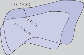
instead of the sequence ![]() . See Figure 6.7 for the time-varying contour.
. See Figure 6.7 for the time-varying contour.
Figure 6.7 Time-varying contour
Setting ![]() , we have
, we have
![]()
The variation of the energy functional Φ is

where rt = ∂r/∂t, rs = ∂r/∂s, n = n(s, t) is the unit normal to the curve ![]() , and T = T(s, t) is the unit tangent vector. Hence, the direction for which Φ(t) decreases most rapidly is given by
, and T = T(s, t) is the unit tangent vector. Hence, the direction for which Φ(t) decreases most rapidly is given by
Decomposing ![]() , equation (6.63) becomes
, equation (6.63) becomes
which means that the curve r(s, t) moves along its normal with speed
6.65 ![]()
Since
![]()
we can determine the update ![]() by
by
6.66 ![]()
![]()
![]()
6.67 ![]()
6.68 ![]()
![]()
6.4.2 Level Set Method
The active contour scheme using the explicit expression ![]() is not appropriate for segmenting multiple targets whose locations are unknown. Using an auxiliary function ϕ(r, t), the propagating contour
is not appropriate for segmenting multiple targets whose locations are unknown. Using an auxiliary function ϕ(r, t), the propagating contour ![]() changing its topology (splitting multiple closed curves) can be expressed effectively by the implicit expression of the zero level set
changing its topology (splitting multiple closed curves) can be expressed effectively by the implicit expression of the zero level set
![]()
With the level set method (Osher et al. 2002), the motion of the active contour with the explicit expression (6.64)) is replaced by the motion of level set. Using the property that
![]()
we have the equation of ϕ containing the embedded motion of ![]() ; for a fixed s,
; for a fixed s,
![]()
Since
![]()
the above identity leads to
6.69 ![]()
Consider the special model:

This can be expressed as
The convection term 〈∇g, ∇ϕ 〉 increases the attraction of the deforming contour toward the boundary of an object. Note that (6.70) is related to the geodesic active contour model (6.64).
The level set method is one of the most widely used segmentation techniques; it can be combined with the problem of minimizing the energy functional of a level set function φ:
6.71 ![]()
where Fitφ is a fitting term for attracting the zero-level contour Cφ: = {φ = 0} toward the target object in the image, Regφ is a regularization term of φ for penalizing non-smoothness of the contour, and μ is the regularization parameter. There exist a variety of fitting models, such as edge-based methods (Caselles et al. 1993, 1997; Goldenberg et al. 2001; Kichenassamy et al. 1995; Malladi et al. 1995), region-based methods (Chan and Vese 2001; Paragios and Deriche 1998; Yezzi et al. 1999), methods based on prior information (Chen et al. 2002) and so on. These fitting models are mostly combined with the standard regularization term penalizing the arc length of the contour Cφ. Among the variety of fitting models, the best-fitting model has to be selected depending on characteristics of the image. The selected fitting model is usually combined with an appropriate regularization term.
For example, Chan and Vese (2001) used the following energy functional (Chan–Vese model):
where λ1 and λ2 are non-negative parameters, ϕ is the level set function, and ave{ϕ≥0} and ave{ϕ<0} are the average values of u(r) in the two-dimensional regions {ϕ < 0} and {ϕ > 0}, respectively. Here, H(ϕ) is the one-dimensional Heaviside function, with H(s) = 1 if s ≥ 0, and H(s) = 0 if s < 0. To compute a minimizer ϕ for the minimization problem (6.72), the following parabolic equation is solved to the steady state:
6.73 ![]()
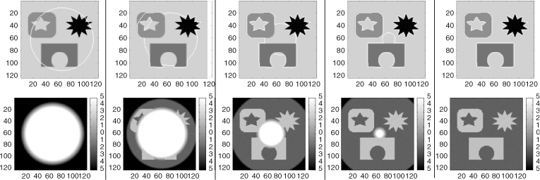
with an appropriate initial level set function. After the evolution comes to a converged state, the zero level set of ϕ becomes the contour that separates the object from the background, as shown in Figure 6.8.
Figure 6.8 Segmentation of different objects with different intensities, with ϕ initialized as a signed distance function. The images at the top show the evolution of the zero level set. The images at the bottom show the evolution of the corresponding level set function. These are the converged results after 323 iterations
6.74 
6.75 ![]()
![]()
6.4.3 Motion Tracking for Echocardiography
Ultrasound imaging is widely used because of its non-invasiveness, real-time monitoring, cost-effectiveness and portability compared with other medical imaging modalities such as CT or MRI. In particular, owing to its high temporal resolution, cardiac ultrasound (echocardiogram) has been very successful in providing a quick assessment of the overall health of the heart. For quantitative assessment of cardiac functions, wall motion tracking and left ventricle (LV) volume quantification at each time are needed. Since manual delineation from echocardiography is extremely labor-intensive and time-consuming, the demands for automated analysis methods are rapidly increasing.
The motion tracking of LV is carried out by observing the speckle pattern associated with deforming tissue. Speckle pattern is inherent appearance in ultrasound imaging and its local brightness reflects the local echogeneity of the underlying scatterers. Since it is a difficult task to automatically track the motion of the endocardial border in ultrasound images because of the poor image quality, low contrast and edge dropout by weak signals, some user intervention is required for stable and successful tracking of the endocardial border.
The most commonly used method for motion tracking is optical flow methods, which use the assumption that the intensity of a moving object is constant over time. If I(r, t) represents the intensity of echocardiography at the location r = (x, y) and the time t, a voxel at (r, t) will move by Δr between two image frames that are taken at times t and t + Δt:
![]()
From Taylor's expansion, the time-varying images I(r, t) approximately satisfy
![]()
Hence, the displacement vector (or velocity vector) u(r, t) to be estimated is governed by
Based on (6.76), numerous approaches for estimating the velocity vector u(r, t) have been proposed and have been applied to LV border tracking in echocardiography (Duan et al. 2009; Linguraru et al. 2008; Suhling et al. 2005; Veronesi et al. 2006).
Horn and Schunk (1981) proposed an optical flow technique that incorporates the smoothness of the motion vector in the entire image as a global constraint. In their model, the velocity u(r, t) at each time t is determined by minimizing the energy functional:
6.77 ![]()
where Ω is the image domain and λ is a regularization parameter that controls the balance between the optical flow term and the smoothness on u. The velocity u(r, t) at each time t can be computed by solving the corresponding Euler–Lagrange equation, which is a reaction–diffusion equation. Barron et al. (1994) observed that this global method with the global smoothness constraint is significantly more sensitive to noise than the local method used by Lucas and Kanade (1981).
Lucas and Kanade (1981) used the assumption of locally constant motion to compute the velocity u(r0, t) at a target location r0 = (x0, y0) and time t by forcing a constant velocity in a local neighborhood of a point r0 = (x0, y0), denoted by ![]() . They estimated the velocity u(r0, t) by minimizing the weighted least-squares criterion in the neighborhood
. They estimated the velocity u(r0, t) by minimizing the weighted least-squares criterion in the neighborhood ![]() :
:
where w is a weight function that enables more relevance to be given to central terms rather than the ones in the periphery. Since this method determines u(r0, t) at each location r0 by combining information from all pixels in the neighborhood of r0, it is reasonably robust against image noise.
Let us explain the numerical algorithm for the Lucas–Kanade method. We denote the endocardial border traced at an initially selected frame (for example, end-systole or end-diastole frame) by a parametric contour ![]() that can be identified as its n control points
that can be identified as its n control points ![]() . Here, we have 0 = s1 < s2 < ··· < sn = 1. Let
. Here, we have 0 = s1 < s2 < ··· < sn = 1. Let ![]() be the contour deformed from
be the contour deformed from ![]() at time t. The motion of the contour
at time t. The motion of the contour ![]() will be determined by an appropriately chosen velocity Ut indicating a time change of control points (r1(t), …, rn(t)):
will be determined by an appropriately chosen velocity Ut indicating a time change of control points (r1(t), …, rn(t)):

Here, we identify the contour ![]() with control points (r1(t), …, rn(t)).
with control points (r1(t), …, rn(t)).
In the Lucas–Kanade method, U(t) for each time t is a minimizer of the energy functional:
To derive the Euler–Lagrange equation from (6.79), we take the partial derivative of ![]() with respect to each uj:
with respect to each uj:
For a numerical algorithm, we replace the integral over ![]() by summation over pixels around rj(t). Assuming that the neighborhood
by summation over pixels around rj(t). Assuming that the neighborhood ![]() consists of m pixels rj1, …, rjm, equation (6.80) becomes
consists of m pixels rj1, …, rjm, equation (6.80) becomes
6.81 ![]()
where Aj = [∇I(rj1, t), …, ∇I(rjm, t)]T, ![]() and bj = [It(rj1, t), …, It(rjm, t)]T. As we mentioned before, there often exist some incorrectly tracked points due to weak signals on the cardiac wall, since echocardiography data are acquired through transmitting and receiving ultrasound signals between the ribs, causing considerable shadowing of the cardiac wall (Leung et al. 2011). Owing to these incorrectly tracked points, the Lucas–Kanade method may produce a distorted LV shape.
and bj = [It(rj1, t), …, It(rjm, t)]T. As we mentioned before, there often exist some incorrectly tracked points due to weak signals on the cardiac wall, since echocardiography data are acquired through transmitting and receiving ultrasound signals between the ribs, causing considerable shadowing of the cardiac wall (Leung et al. 2011). Owing to these incorrectly tracked points, the Lucas–Kanade method may produce a distorted LV shape.
6.82 
6.83 
1 For hydrogen 1H, γ = 2π × 42.576 × 106 rad s−1 T−1.
References
Aubert G and Kornprobst P 2002 Mathematical Problems in Image Processing: Partial Differential Equations and the Calculus of Variations, 2nd edn. Applied Mathematical Sciences Series, vol. 147. Springer, New York.
Barron JL, Fleet DJ and Beauchemin SS 1994 Performance of optical flow techniques. Int. J. Comput. Vision 12(1), 43–77.
Beer 1852 Bestimmung der Absorption des rothen Lichts in farbigen Flussigkeiten. Ann. Phys. Chem. 86, 78–88.
Bracewell RN 1956 Strip integration in radioastronomy. J. Phys. 9, 198–217.
Bracewell RN and Riddle AC 1967 Inversion of fan-beam scans in radio-astronomy. Astrophys. J. 150, 427–434.
Brooks RA and Chiro GD 1976 Beam hardening in x-ray reconstructive tomography. Phys. Med. Biol. 21, 390–398.
Bydder M, Larkman DJ and Hajnal JV 2002 Generalized SMASH imaging. Magn. Reson. Med. 47, 160–170.
Calder J and Mansouri A 2011 Anisotropic image sharpening via well-posed Sobolev gradient flows. SIAM J. Math. Anal. 43, 1536–1556.
Candès EJ and Tao T 2005 Decoding by linear programming. IEEE Trans. Inform. Theory 51(12), 4203–4215.
Candès EJ and Tao T 2006 Near-optimal signal recovery from random projections: universal encoding strategies. IEEE Trans. Inform. Theory 52, 5406–5425.
Candès EJ, Romberg J and Tao T 2006a Robust uncertainty principles: exact signal reconstruction from highly incomplete frequency information. IEEE Trans. Inform. Theory 52(2), 489–509.
Candès EJ, Romberg JK and Tao T 2006b Stable signal recovery from incomplete and inaccurate measurements. Commun. Pure Appl. Math. 59, 1207–1223.
Canny JA 1986 Computational approach to edge detection. IEEE Trans. Pattern Anal. Machine Intell. 8(6), 679–698.
Caselles V, Catte F, Coll T and Dibos F 1993 A geometric model for active contours in image processing. Numer. Math. 66(1), 1–31.
Caselles V, Kimmel R and Sapiro G 1997 Geodesic active contours. Int. J. Comput. Vision 22(1), 61–79.
Chan TF and Vese LA 2001 Active contours without edges. IEEE Trans. Image Process. 10(2), 266–277.
Chen Y, Tagare HD, Thiruvenkadam S, Huang F, Wilson D, Gopinath KS, Briggs RW and Geiser EA 2002 Using prior shapes in geometric active contours in a variational framework. Int. J. Comput. Vision 50(3), 315–328.
Cormack AM 1963 Representation of a function by its line integrals, with some radiological applications. J. Appl. Phys. 34, 2722–2727.
Cormack AM 1992 75 years of radon transform. J. Comput. Assist. Tomogr. 16, 673.
Damadian RV 1971 Tumor detection by nuclear magnetic resonance. Science 171, 1151–1153.
Donoho DL and Elad M 2003 optimally sparse representation in general (non-orthogonal) dictionaries via ![]() 1 minimization. Proc. Natl Acad. Sci. USA 100, 2197–2202.
1 minimization. Proc. Natl Acad. Sci. USA 100, 2197–2202.
Donoho DL and Huo X 1999 Uncertainty principles and ideal atomic decomposition. IEEE Trans. Inform. Theory 47, 2845–2862.
Duan Q, Angelini ED, Herz SL, Ingrassia CM, Costa KD, Holmes JW, Homma S and Laine AF 2009 Region-based endocardium tracking on real-time three-dimensional ultrasound. Ultrasound Med. Biol. 35(2), 256–265.
Faridani A 2003 Introduction to the mathematics of computed tomography. In Inside Out: Inverse Problems and Applications (ed. G Uhlmann). Math. Sci. Res. Inst. Publications, vol. 47, pp. 1–46. Cambridge University Press, Cambridge.
Feldkamp LA, Davis LC and Kress JW 1984 Practical cone-beam algorithm. J. Opt. Soc. Am. A 1(6), 612–619.
Filler AG 2010 The history, development, and impact of computed imaging in neurological diagnosis and neurosurgery: CT, MRI, DTI Internet J. Neurosurg. 7(1).
Goldenberg R, Kimmel R, Rivlin E and Rudzsky M 2001 Fast geodesic active contours. IEEE Trans. Image Process. 10(10), 1467–1475.
Grangeat P 1991 Mathematical framework of cone beam 3D reconstruction via the first derivative of the Radon transform. In Mathematical Methods in Tomography (Oberwolfach, 1990). Lecture Notes in Mathematics, no. 1497, pp. 66–97. Springer, Berlin.
Griswold MA, Jakob PM, Heidemann RM, Nittka M, Jellus V, Wang J, Kiefer B and Haase A 2002 Generalized autocalibrating partially parallel acquisitions (GRAPPA). Magn. Reson. Med. 47, 1202–1210.
Haacke E, Brown R, Thompson M and Venkatesan R 1999 Magnetic Resonance Imaging Physical Principles and Sequence Design. John Wiley & Sons, Inc., New York.
Heidemann RM, Griswold MA, Haase A and Jakob PM 2001 VD-AUTO-SMASH imaging. Magn. Reson. Med. 45, 1066–1074.
Horn B and Schunk B 1981 Determining optical flow. Artif. Intell. 17(2), 185–203.
Hounsfield GN 1973 Computerized transverse axial scanning (tomography): I. Description of system. Br. J. Radiol. 46, 1016–1022.
Jakob PM, Griswold MA, Edelman RR and Sodickson DK 1998 AUTO-SMASH: a self-calibrating technique for SMASH imaging. Magn. Reson. Mater. Phys., Biol. Med. 7, 42–54.
Kak AC and Slaney M 1988 Principles of Computerized Tomographic Imaging. IEEE Press, New York.
Kalender WA 2006 X-ray computed tomography. Phys. Med. Biol. 51, R29–R43.
Kalender WA, Hebel R and Ebersberger J 1987 Reduction of CT artifacts caused by metallic implants. Radiology 164(2), 576–577.
Kass M, Witkin A and Terzopoulos D 1987 Snake: active contour models. Int. J. Comput. Vision 1, 321–331.
Kichenassamy S 1997 The Perona–Malik paradox. SIAM J. Appl. Math. 57(5), 1328–1342.
Kichenassamy S, Kumar A, Olver P, Tannenbaum A and Yezzi A 1995 Gradient flows and geometric active contour models. In Proc. 5th Int. Conf. on Computer Vision, pp. 810–815. IEEE Press, New York.
Kyriakos WE, Panych LP, Kacher DF, Westin CF, Bao SM, Mulkern RV and Jolesz FA 2000 Sensitivity profiles from an array of coils for encoding and reconstruction in parallel (SPACE RIP). Magn. Reson. Med. 44, 301–308.
Lambert JH 1760 Photometria, sive de Mensura et gradibus luminis,colorum et umbrae. Eberhardt Klett, Augsburg.
Larkman DJ and Nunes RG 2001 Parallel magnetic resonance imaging. Phys. Med. Biol. 52, R15.
Lauterbur PC 1973 Image formation by induced local interactions: examples of employing nuclear magnetic resonance. Nature 242(5394), 190–191.
Lauterbur PC 1974 Magnetic resonance zeugmatography. Pure Appl. Chem. 40, 149–157.
Leung KY, Danilouchkine MG, Stralen MV, Jong NE, Steen AFVD and Bosch JG 2011 Left ventricular border tracking using cardiac motion models and optical flow. Ultrasound Med. Biol. 37(4), 605–616.
Linguraru MG, Vasilyev NV, Marx GR, Tworetzky W, Nido PJD and Howe RD 2008 Fast block flow tracking of atrial septal defects in 4D echocardiography. Med. Image Anal. 12(4), 397–412.
Lucas B and Kanade T 1981 An iterative image restoration technique with an application to stereo vision. Proc. DARPA Image Understanding Workshop, pp. 121–130.
Lustig M, Donoho DL and Pauly JM 2007 Sparse MRI: the application of compressed sensing for rapid MR imaging. Magn. Reson. Med. 58, 1182–1195.
Malladi R, Sethian JA and Vemuri BC 1995 Shape modeling with front propagation: a level set approach. IEEE Trans. Pattern Anal. Machine Intell. 17(2), 158–175.
Meyer Y Oscillating Patterns in Image Processing and Nonlinear Evolution Equations. University Lecture Series, vol. 22. American Mathematical Society, Providence, RI.
Meyer E, Raupach R, Lell M, Schmidt B and Kachelrie M 2010 Normalized metal artifact reduction (NMAR) in computed tomography. Med. Phys. 37, 5482–5493.
Natterer F 2008 X-Ray Tomography, Inverse Problems and Imaging. Lecture Notes in Mathematics, no. 1943, pp. 17–34. Springer, Berlin.
Osher S, Solé A and Vese L 2002 Image decomposition and restoration using total variation minimization and the H−1 norm. SIAM Multiscale Model. Simul. 1(3), 349–370.
Osher S, Burger M, Goldfarb D, Xu J and Yin W 2005 An iterative regularization method for total variation-based image restoration. SIAM Multiscale Model. Simul. 4(2), 460–489.
Paragios N and Deriche R 1998 A PDE-based level set approach for detection and tracking of moving objects. In Proc. 6th Int. Conf. on Computer Vision, pp. 1139–1145. IEEE, New York.
Perona P and Malik J 1990 Scale space and edge detection using anisotropic diffusion. IEEE Trans. Pattern Anal. Machine Intell. 12, 629–639.
Pruessmann KP, Weiger M, Scheidegger MB and Boesiger P 1999 SENSE: sensitivity encoding for fast MRI. Magn. Reson. Med. 42, 952–962.
Pruessmann KP, Weiger M, Bornert P and Boesiger P 2001 Advances in sensitivity encoding with arbitrary k-space trajectories. Magn. Reson. Med. 46, 638–651.
Radon JH 1917 Über die Bestimmung von Funktionen durch ihre Integralwerte längs gewisser Mannigfaltigkeiten. Ber. Sächs. Akad. Wiss. (Leipzig) 69, 262–277.
Rudin L, Osher SJ and Fatemi E 1992 Nonlinear total variation based noise removal algorithms. Physica D 60, 259–268.
Sarti A, Corsi C, Mazzini E and Lamberti C 2005 Maximum likelihood segmentation of ultrasound images with Rayleigh distribution. IEEE Trans. Ultrason. Ferroelectr. Freq. Control 52(6), 947–960.
Sodickson DK and Manning WJ 1997 Simultaneous acquisition of spatial harmonics (SMASH): fast imaging withradiofrequency coil arrays. Magn. Reson. Med. 38, 591–603.
Sodickson DK, Griswold MA, Jakob PM, Edelman RR and Manning WJ 1999 Signal-to-noise ratio and signal-to-noise efficiency in SMASH imaging. Magn. Reson. Med. 41, 1009–1022.
Suhling M, Arigovindan M, Jansen C, Hunziker P and Unser M 2005 Myocardial motion analysis from B-mode echocardiograms. IEEE Trans. Image Process. 14(4), 525–536.
Tuy HK 1983 An inversion formula for cone-beam reconstruction. SIAM J. Appl. Math. 43, 546–552.
Veronesi F, Corsi C, Caiani EG, Sarti A and Lamberti C 2006 Tracking of left ventricular long axis from real-time three-dimensional echocardiography using optical flow techniques. IEEE Trans. Inform. Technol. Biomed. 10(1), 174–181.
Vese L and Osher S 2002 Modeling textures with total variation minimization and oscillating patterns in image processing. J. Sci. Comput. 19, 553–572.
Wang G, Snyder DL, O'Sullivan JA and Vannier MW 1996 Iterative deblurring for CT metal artifact reduction. IEEE Trans. Med. Imag. 15, 657–664.
Weickert J 1997 A review of nonlinear diffusion filtering. In Scale-Space Theory in Computer Vision (eds BtH Romeny, L Florack, J Koenderink and M Viergever). Lecture Notes in Computer Science, no. 1252, pp. 3–28. Springer, Berlin.
Yezzi A, Tsai A and Willsky A 1999 Binary and ternary flows for image segmentation. In Proc. Int. Conf. on Image Processing, vol. 2, pp. 1–5. IEEE, New York.
You Y, Xu W, Tannenbaum A and Kaveh M 1996 Behavioral analysis of anisotropic diffusion in image processing. IEEE Trans. Image Process. 5, 15–53.
Further Reading
Aubert G and Vese L 1997 A variational method in image recovery. SIAM J. Numer. Anal. 34(5), 1948–1979.
Candès EJ and Tao T 2008 Reflections on compressed sensing. IEEE Inform. Theory Soc. Newslett. 58, 20–23.
Carr HY 2004 Field gradients in early MRI. Physics Today 57(7), 83.
Donoho DL 2006 Compressed sensing. IEEE Trans. Inform. Theory 52(4), 1289–1306.
McLachlan GJ and Peel D Finite Mixture Models. Wiley Series in Probability and Statistics, no. 84. John Wiley & Sons, Inc., New York.
Mumford D and Shah J 1989 Optimal approximation by piecewise smooth functions and associated variational problems. Commun. Pure Appl. Math. 42, 577–685.
Osher S and Fedkiw R 2002 Level Set Methods and Dynamic Implicit Surfaces. Springer, New York.
Zhao HK, Chan T, Merriman B and Osher S 1996 A variational level set approach to multiphase motion. J. Comput. Phys. 127, 179–95.


