Chapter 10
Magnetic Resonance Elastography
Magnetic resonance elastography (MRE) is an imaging modality capable of visualizing the stiffness of biological tissues by measuring the propagating strain waves in an object of interest (Low et al. 2010; Muthupillai et al. 1995; Papazoglou et al. 2005; Sack et al. 2002; Sinkus et al. 2000). Since MRE provides non-invasive assessment of variations in tissue elasticity, it has been used for non-invasive diagnosis of liver disease or for detecting prostate cancer. Tissue elasticity can change with disease, and the shear modulus (or modulus of rigidity) varies over a wide range, differentiating various pathological states of tissues (Venkatesh et al. 2008; Yin et al. 2007). It also has potential applications in studying skeletal muscle biomechanics (Papazoglou et al. 2005; Uffmann et al. 2004).
Tissue elasticity refers to the ability of a tissue to deform its shape when a mechanical force is applied and to regain its original shape after the force is removed; tumor tissue is less compressible than normal tissue. For centuries, palpation using the surface of the finger or palm has been used to measure tissue stiffness; it can be viewed as an elasticity measurement technique to feel the degree of tissue distortion (strain) due to pressure (stress) on the tissue. As a visual palpation, elastography using ultrasound was developed in the late 1980s (Lerner and Parker 1987; Ophir et al. 1991). This ultrasound elastography influenced the early development of MRE.
MRE provides a quantitative assessment of tissue stiffness (shear modulus) with a non-invasive method. It is based on the fact that the speed of shear wave propagation is closely related to tissue stiffness; the stiffer the tissue, the faster the speed. For a linear elastic medium, the shear modulus is proportional to the square of the shear velocity. To measure the shear velocity, MRE uses magnetic resonance imaging (MRI) techniques to detect the propagation of transverse acoustic strain waves in the object of interest (Muthupillai et al. 1995). It visualizes the time-harmonic displacement in the tissue induced by a harmonically oscillating mechanical vibration. With a fixed frequency, the shear velocity is proportional to the wavelength, which can be viewed as the peak-to-peak distance of the time-harmonic displacement. Hence, we can evaluate local values of tissue elasticity from the time-harmonic displacement. We refer to the review articles of Doyley (2012) and Mariappan et al. (2010) for overviews of MRE techniques. In this chapter, we will introduce several MRE approaches, from basic physics to potential applications.
10.1 Representation of Physical Phenomena
When a force is applied to a solid body, the body deforms in shape and volume to some extent. If the deformed body returns to its original shape once the force is removed, it is said to have experienced elastic deformation. If the deformation is irreversible, it is said to be plastic deformation. Stress is a description of the average force per unit normal area of a surface within a body. The unit of stress is the pascal (Pa = N m2, newtons per square meter). Strain measures the extent of deformation in terms of a relative displacement, that is, the change of distance between two adjacent points in the deformed state with respect to that distance in the undeformed state. In this section, we will deal only with linear elastic materials, and we give a brief overview of some elementary concepts in linear elasticity regarding the relationship between stress and strain. We refer to the books of Landau and Lifshitz (1986) and Pujol (2002) for detailed explanations.
10.1.1 Overview of Hooke's Law
Hooke's law states that strain is proportional to stress. In a one-dimensional simple model of a rod of elastic material,
10.1 ![]()
where E is Young's modulus. Here, we regard the rod of elastic material as a spring; Young's modulus can be viewed as the spring constant. Young's modulus E = σ/![]() can be used to predict compression or elongation as a result of axial stress. A compressive force causes the rod to get shorter, whereas a tensile force makes the rod longer.
can be used to predict compression or elongation as a result of axial stress. A compressive force causes the rod to get shorter, whereas a tensile force makes the rod longer.
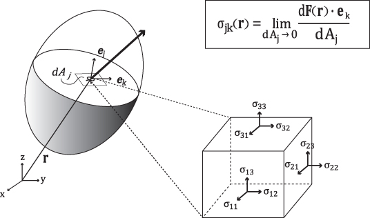
A generalized Hooke's law for a three-dimensional elastic body can be derived by viewing the elastic body as a network of linear springs. For a three-dimensional inhomogeneous elastic body, the stress at any given point r within the body is defined by a 3 × 3 matrix called the Cauchy stress tensor:

The first column of the stress tensor ![]() represents the force acting on a differential area dA normal to the x axis (see Figure 10.1). Similarly, the second and third columns of
represents the force acting on a differential area dA normal to the x axis (see Figure 10.1). Similarly, the second and third columns of ![]() are the forces acting on the differential area dA normal to the y and z axes, respectively. There are three main types of stress: compression, tension and shear stress. The diagonal components σ11, σ22 and σ33 are normal stresses, the forces perpendicular to the area dA. The remaining off-diagonal components are shear stresses, the forces parallel to the area dA.
are the forces acting on the differential area dA normal to the y and z axes, respectively. There are three main types of stress: compression, tension and shear stress. The diagonal components σ11, σ22 and σ33 are normal stresses, the forces perpendicular to the area dA. The remaining off-diagonal components are shear stresses, the forces parallel to the area dA.
Figure 10.1 Stress tensor
Strain can be obtained by comparing deformed geometry with undeformed geometry. The strain at any given point r within the body is expressed by the 3 × 3 matrix

Then, the generalized three-dimensional Hooke's law can be expressed as
where C = (Cijk![]() ) is the fourth-order elastic tensor, which is symmetrical: Cijk
) is the fourth-order elastic tensor, which is symmetrical: Cijk![]() = Cij
= Cij![]() k = Cjik
k = Cjik![]() . The tensor (Cijk
. The tensor (Cijk![]() ) is called the stiffness tensor, and it links the stress tensor and the strain tensor.
) is called the stiffness tensor, and it links the stress tensor and the strain tensor.
Adopting the Voigt notation (e.g. C1123 = C14), we can rewrite (10.2) in the following matrix representation:
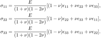
In the case of isotropic materials, (10.3) can be simplified as
with
![]()
where E is Young's modulus, ν is Poisson's ratio and μ is the shear modulus.
Next, we will briefly describe the derivation of (10.4) by considering a cubic material aligned with the axes {x, y, z}. We assume that three “tension tests”, labeled as ′, ′′ and ′′′, are conducted along x, y and z, respectively. Then, normal strains will be produced as follows:

The combined strains can be obtained by superposition:

This provides us with the three equations
The shear strains and stresses are connected by the shear modulus μ as
![]()
where
![]()
which leads to
The identity (10.4) follows from (10.5) and (10.6).
10.7 
10.1.2 Strain Tensor in Lagrangian Coordinates
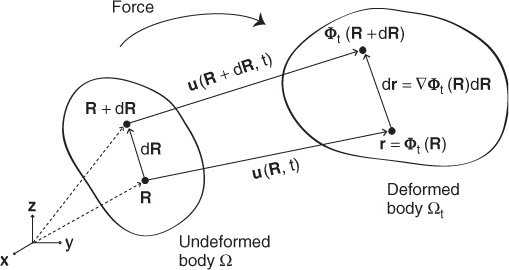
We now provide basic descriptions of the strain tensor. Let Φt:Ω → Ωt be the mapping from the undeformed body Ω at time t = 0 to the deformed state Φt(Ω) = Ωt at time t. Let R = (X, Y, Z) denote a position of a particle in the undeformed frame, and let r = r(R, t) = Φt(R) indicate the position of the same particle in the deformed frame at time t (see Figure 10.2). Hence, the motion of the specified particle at R in the reference frame is described by r(R, t) = Φt(R). This approach is called the Lagrangian description. One may use the Eulerian description R = R(r, t) when we are interested in a particle that occupies a given point r at a given time.
Figure 10.2 Relative particle movement in the continuum
The displacement vector (the total movement of a particle with respect to the undeformed frame) is given by
![]()
With the assumption of small deformations, we can approximate
![]()
where I is the identity matrix and ![]() is the 3 × 3 matrix
is the 3 × 3 matrix

To analyze the change in length elements, we compare the distance |dr|2 in the deformed frame with the distance |dR|2 in the reference frame:
![]()
From the assumption of small deformations, we can neglect the term ![]() to get the approximation
to get the approximation
![]()
Introducing Cauchy's infinitesimal strain tensor
![]()
the difference |dr|2 − |dR|2 can be approximated by
![]()
Since |dr|2 − |dR|2 ≈ 2|dR|(|dr| − |dR|), the relative change in length in the dR direction is
![]()
The above identity provides some geometric meaning of the strain tensor.
10.2 Forward Problem and Model
Newton's second law (force = mass × acceleration) provides a description of motion. We will use the Eulerian description of motion in order to focus on a particle at r = r(R, t). As t varies, different particles occupy the same spatial point r. With the Eulerian description, the velocity v = ∂u(R, t)/∂t can be expressed as
![]()
Here, D/Dt is the derivative with respect to time t keeping R constant (called the material derivative), and ∂/∂t is the derivative with respect to time t keeping r constant. Similarly, the acceleration of a particle can be expressed as
![]()
Assuming that the density of the body, denoted by ρ, is locally constant, let us examine the equation of motion in a small cube Q with surface ∂Q. From the balance of linear momentum,
where n is the unit outward normal vector and f is the body force per unit volume. From the divergence theorem, (10.8) becomes
10.9 ![]()
Since the cube Q is arbitrarily small, (10.8) leads to
From the assumption of small deformations, the acceleration Dv/Dt is approximated by

Assuming that the body is isotropic, the generalized Hooke's law (10.2) leads to
where μ and λ are the Lamé coefficients given by
![]()
with Poisson's ratio ν. Hence, substituting (10.11) into (10.10) yields the equation of motion in terms of the displacement u:
In the case of a locally homogeneous isotropic medium, (10.12) can be simplified to
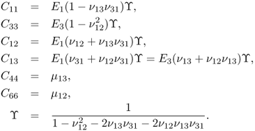
In the case of an anisotropic medium, u = (u1, u2, u3) is dictated by the following elasticity system (Landau and Lifshitz 1986):
10.3 Inverse Problem in MRE
Imaging methods in MRE can be roughly divided into three steps (Mariappan et al. 2010):
- Excitation. Apply a sinusoidal vibration with an angular frequency of oscillation
 ,
,  through the surface of the object. This induces tissue vibrations in an imaging region inside the human body.
 - Tissue response measurement. Measure the induced tissue vibrations that are magnetically encoded by oscillating magnetic field gradients (Muthupillai et al. 1995).
- Shear modulus reconstruction. Visualize the shear modulus distribution using the measured tissue-displacement field.
The sinusoidal excitation at the angular frequency ![]() induces the internal displacement u(r, t) within the body at the same angular frequency
induces the internal displacement u(r, t) within the body at the same angular frequency ![]() , and its time-harmonic displacement u(x) is given by
, and its time-harmonic displacement u(x) is given by
![]()
Here, for simplicity, we use the same notation for the time-harmonic displacement u(x) as the time-dependent displacement u(r, t). Hopefully, this will not cause any confusion from the context. From now on, the notation u will be used for the time-harmonic displacement. Assume that ρf ≈ 0 in (10.13) and (10.14).
For a linear isotropic body, substituting ![]() into (10.13) leads to the governing equation of the induced internal time-harmonic displacement vector u:
into (10.13) leads to the governing equation of the induced internal time-harmonic displacement vector u:
Here, taking the viscosity effect into account, μ and λ can be complex-valued. The real part ![]() is the shear modulus and
is the shear modulus and ![]() is the Lamé coefficient, with
is the Lamé coefficient, with
![]()
![]() is the shear viscosity accounting for attenuation within the medium and
is the shear viscosity accounting for attenuation within the medium and ![]() is the viscosity of the compressible wave.
is the viscosity of the compressible wave.
Similarly, in the case of an anisotropic material, substituting ![]() into (10.14) with
into (10.14) with ![]() leads to
leads to
The corresponding inverse problem is to recover the distribution of tissue elasticity from the time-harmonic displacement u(r) inside the body.
10.4 Reconstruction Algorithms
Let Ω be the domain occupying the object to be imaged. Assume that soft tissues exhibit linear, isotropic mechanical properties. Most reconstruction methods for shear modulus imaging have used the following scalar equation:
This model has the major advantage of requiring one component of u, and it simplifies the underlying mathematical theory to the corresponding inverse problem; the inverse problem using the vector equation (10.15) can be reduced to the inverse problem using the scalar equation (10.17). We refer the interested reader to Manduca et al. (2001), McLaughlin and Renzi (2006), McLaughlin and Yoon (2004), Oliphant et al. (2001) and Sinkus et al. (2005b).
This model (10.17) uses the assumption that the longitudinal wave can be filtered out, since the longitudinal wave varies slowly compared with the shear wave (McLaughlin and Renzi 2006; Sinkus et al. 2005b). We should note that the scalar equation (10.17) for u is not accurate because ![]() is not negligible; although
is not negligible; although ![]() is very small, λ is very large. However, it seems that the scalar equation (10.17) for μ is reasonably accurate; for a given axial component of time-harmonic shear wave in (10.15), the shear modulus μ approximately satisfies (10.17).
is very small, λ is very large. However, it seems that the scalar equation (10.17) for μ is reasonably accurate; for a given axial component of time-harmonic shear wave in (10.15), the shear modulus μ approximately satisfies (10.17).
The scalar equation (10.17) can be derived under the assumptions that ![]() and
and ![]() are small (Lee et al. 2010). From the elasticity equation (10.15), u can be decomposed into
are small (Lee et al. 2010). From the elasticity equation (10.15), u can be decomposed into
where

Neglecting ϒ ≈ 0, we get the following approximation:

Writing
![]()
the decomposition (10.19) is expressed as
10.20 ![]()
Application of divergence to both sides of (10.19) leads to
10.21 ![]()
Since ![]() , the above approximation yields
, the above approximation yields ![]() . Therefore, uL satisfies both
. Therefore, uL satisfies both ![]() and
and ![]() . This means that each component of uL satisfies the Laplace equation approximately
. This means that each component of uL satisfies the Laplace equation approximately
From the elasticity equation (10.15) with the assumptions ![]() and
and ![]() , we have
, we have
10.23 ![]()
From (10.22), uL is approximately harmonic in the region of interest, thereby varying very slowly in the internal region with negligible contribution to u. Hence, uL can be treated as noise in the data (McLaughlin and Renzi 2006) and we may assume that the shear modulus μ and the displacement u satisfy the forward equation
For the above derivation of (10.24), we have used the assumption of ![]() in two places.
in two places.
10.4.1 Reconstruction of μ with the Assumption of Local Homogeneity
Assuming local homogeneity on μ (or ![]() ), (10.24) can be expressed as
), (10.24) can be expressed as
Then, μ can be directly recovered from
This direct inversion method is the most commonly used MRE algorithm, which requires the local homogeneity assumption on μ (Kruse et al. 2000; Manduca et al. 2001; Manduca et al. 2002; Manduca et al. 2003; Oliphant et al. 2000a; Oliphant et al. 2000b; Oliphant et al. 2001; Sinkus et al. 2005b). Figure 10.3 shows the performance of the direct algebraic inversion method (Mariappan et al. 2010).
Figure 10.3 Typical MR elastograms. Reproduced from the GE Healthcare website at http://www.gehealthcare.com/euen/mri/products/MR-Touch/index.html
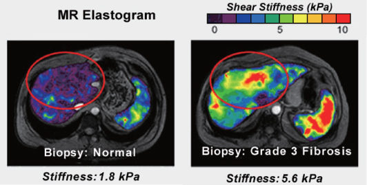
One drawback of the direct algebraic inversion method (10.26) is that double differentiation of the measured displacement data u can cause undesirable noise effects owing to the tendency of the operation to amplify noise. To alleviate the noise amplification from measured data, this method typically needs some filtering to reduce high-frequency noise (Manduca et al. 2003). Another drawback of this method is that the modeling error from the assumption of local homogeneity produces artifacts around regions of differing elastic properties even with noiseless data (Kwon et al. 2009).
10.4.2 Reconstruction of μ without the Assumption of Local Homogeneity
Next, we explain a method for reconstructing shear modulus images without the assumption of local homogeneity (Kwon et al. 2009; Lee et al. 2010).
According to the Helmholtz–Hodge decomposition, the vector field ![]() in (10.17) can be decomposed into a curl-free component and a divergence-free component:
in (10.17) can be decomposed into a curl-free component and a divergence-free component:
where the scalar potential f satisfies
and the vector field W satisfies
Taking the inner product of ![]() , the complex conjugate of
, the complex conjugate of ![]() , on both sides of the identity (10.27) leads to the following identity:
, on both sides of the identity (10.27) leads to the following identity:
10.30 ![]()
Assuming ![]() , μ can be decomposed into
, μ can be decomposed into
where
Let μd denote the recovered shear modulus using the direct inversion formula (10.26):
![]()
The following theorem provides some characteristics of μ* and μd.
![]()

![]()
![]()
![]()
![]()
![]()
10.34 ![]()
![]()
For the image reconstruction, the first quantity μ* in (10.31) can be computed explicitly by solving the problem (10.28) from knowledge of ![]() and the Neumann boundary condition. However, we cannot compute μ** directly since the equation contains the unknown quantity
and the Neumann boundary condition. However, we cannot compute μ** directly since the equation contains the unknown quantity ![]() . Hence, we need an iterative procedure to get μ**. We summarize the reconstruction procedure with the iterative method.
. Hence, we need an iterative procedure to get μ**. We summarize the reconstruction procedure with the iterative method.
- Initial guess
 .
. - For each n = 1, 2, …, compute the vector potential Wn that is the solution of the elliptic equation
10.35 ![]()
- Update
10.36 ![]()
We can test the iterative method via numerical simulations using a rectangular two-dimensional model of 10 × 10 cm2 with the origin at its bottom-left corner. Figure 10.4(a) shows the image of the simulated target shear modulus. The target shear modulus included vertical and lateral thin bars with shear storage modulus ![]() with 0.2 kPa viscosity and background shear storage modulus
with 0.2 kPa viscosity and background shear storage modulus ![]() with 0.1 kPa viscosity. To get the displacement data, we solved the wave equation in (10.25) with the boundary conditions given by u(x, y) = 1 for y = 10, 0 ≤ x ≤ 10 and
with 0.1 kPa viscosity. To get the displacement data, we solved the wave equation in (10.25) with the boundary conditions given by u(x, y) = 1 for y = 10, 0 ≤ x ≤ 10 and ![]() otherwise. Figure 10.4(b) and (c) show the real and imaginary parts of the simulated displacement image, respectively. Figure 10.5(a) and (b) show the intensity of
otherwise. Figure 10.4(b) and (c) show the real and imaginary parts of the simulated displacement image, respectively. Figure 10.5(a) and (b) show the intensity of ![]() and
and ![]() , respectively. Since the wave propagates from the top to bottom, Figure 10.5(a) highlights ∂μ/∂y and Figure 10.5(b) emphasizes ∂μ/∂x.
, respectively. Since the wave propagates from the top to bottom, Figure 10.5(a) highlights ∂μ/∂y and Figure 10.5(b) emphasizes ∂μ/∂x.
Figure 10.4 Simulation set-up. (a) Target shear modulus image. (b) and (c) Simulated real and imaginary displacement images, respectively. From Lee et al. (2010)

Figure 10.5 (a) Simulated image of ![]() and (b) simulated image of
and (b) simulated image of ![]() . From Lee et al. (2010)
. From Lee et al. (2010)
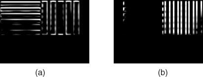
Figure 10.6 shows the reconstructed image of the shear storage moduli μd, μ* and ![]() . The quantity μ* itself is a good approximation of the true μ, as shown in Figure 10.6. The reconstructed μ* was close to the target μ in the left region where
. The quantity μ* itself is a good approximation of the true μ, as shown in Figure 10.6. The reconstructed μ* was close to the target μ in the left region where ![]() and the updated μ5 recovered the missed information of μ* in the region where the intensity of
and the updated μ5 recovered the missed information of μ* in the region where the intensity of ![]() was high in Figure 10.5(b). The recovered
was high in Figure 10.5(b). The recovered ![]() in Figure 10.6(a), even without added noise, shows some artifacts by neglecting the term
in Figure 10.6(a), even without added noise, shows some artifacts by neglecting the term ![]() in the left region where the intensity of
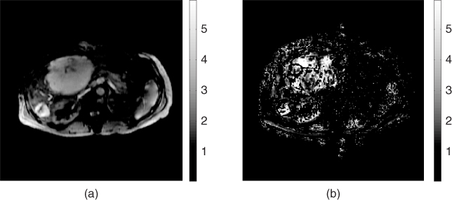
in the left region where the intensity of ![]() was high in Figure 10.4(a). Figure 10.7 shows the results of in vivo human liver experiments (Kwon et al. 2009).
was high in Figure 10.4(a). Figure 10.7 shows the results of in vivo human liver experiments (Kwon et al. 2009).
Figure 10.6 Simulation results. The first column (a), (d) and (g) are the real parts of reconstructed shear modulus using the direct inversion method, with added random noise of 0%, 3%and 6%, respectively. The second and third columns are the real parts of the principal and the fifth-updated shear storage modulus images, respectively, using the shear modulus decomposition algorithm corresponding to the first column. From Lee et al. (2010)
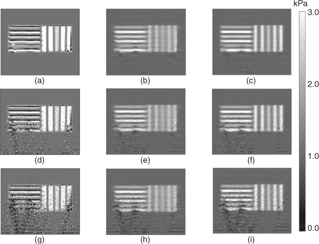
Figure 10.7 Results of in vivo human liver experiments. (a) and (b) Reconstructed shear modulus images using the principal component-based inversion algorithm and the direct inversion algorithm, respectively. From Kwon et al. (2009). Reproduced with permission from IEEE
10.4.3 Anisotropic Elastic Moduli Reconstruction
Most research in MRE has made the assumption that soft tissues exhibit linear and isotropic mechanical properties. However, various biological tissues such as skeletal muscle are known to have anisotropic elastic properties (Chaudhry et al. 2008; Dresner et al. 2001; Gao et al. 1996; Gennisson et al. 2003; Heers et al. 2003; Humphrey 2003; Kruse et al. 2000; McLaughlin et al. 2007). Techniques using the scalar equation (10.17) definitely cannot be applied to such anisotropic cases.
The simplest model of the anisotropy would be a transversely isotropic model. Papazoglou et al. (2005) adopted the model with transverse isotropy in which the principal axis of symmetry x3 = z is aligned to be parallel to the muscle fibers. In this model, the full elasticity system (10.16) is reduced to the two-dimensional elasticity system with elastic moduli (shear modulus, Young's modulus and Poisson's ratio) depending only on r: = (x, z). To be precise, let Ω be the xz plane of the elastic object to be imaged. The time-harmonic displacement wave vector u(r) = (u1(r), u3(r))T, r ∈ Ω, satisfies the following simplified elasticity system:
10.37 
where
![]()
ρ is the tissue density and μβ: = 4μ12E3/E1. Here, E3 and E1 are Young's modulus with respect to the x3 and x1 axes, respectively.
This transversely isotropic model for the elasticity has a potential application of determining the mechanical properties of human skeletal muscle, including the elastic properties of bundles of parallel fibers aligned in one direction. Papazoglou et al. (2005) and Sinkus et al. (2005a) studied this transversely isotropic model with the assumption of local homogeneity. Papazoglou et al. (2005) made a step toward a better description of two-dimensional shear wave patterns to reveal the anisotropy of the muscle fibers. Sinkus et al. (2005a) developed a direct reconstruction scheme for imaging the anisotropic property of breast tissues.
10.5 Technical Issues in MRE
MRE is a non-invasive imaging technique for recovering the mechanical properties of tissues. The image reconstruction algorithm in MRE is not perfect yet, owing to difficulties in handling the general elasticity equations. There are many challenging issues in the inverse problem of MRE. For soft tissues, ![]() is very small, whereas the Lamé parameter λ is very large. Thus, even though
is very small, whereas the Lamé parameter λ is very large. Thus, even though ![]() , the total effect of
, the total effect of ![]() may not be negligible and may produce errors or artifacts in reconstructed images. Hence, it would be desirable to investigate a stable algorithm to reconstruct the Lamé parameters simultaneously without the incompressibility assumption.
may not be negligible and may produce errors or artifacts in reconstructed images. Hence, it would be desirable to investigate a stable algorithm to reconstruct the Lamé parameters simultaneously without the incompressibility assumption.
There have been increasing demands for anisotropic models, but it is very difficult to achieve a robust reconstruction. If MRE alone is insufficient to provide a robust reconstruction of high-resolution images, one may try combining it with other techniques to get some complementary information.
References
Chaudhry H, Bukiet B and Findley T 2008 Mathematical analysis of applied loads on skeletal muscles during manual therapy. J. Am. Osteopath Assoc. 108, 680–688.
Doyley MM 2012 Topical review: Model-based elastography: a survey of approaches to the inverse elasticity problem. Phys. Med. Biol. 57, R35.
Dresner MA, Rose GH, Rossman PJ, Muthupillai R, Manduca A and Ehman RL 2001 Magnetic resonance elastography of skeletal muscle. J. Magn. Reson. Imag. 13, 269–276.
Gao L, Parker KJ, Lerner RM and Levinson SF 1996 Imaging of the elastic properties of tissue—a review. Ultrasound Med. Biol. 22, 959–977.
Gennisson JL, Catheline S, Chaffai S and Fink M 2003 Transient elastography in anisotropic medium: application to the measurement of slow and fast shear wave speeds in muscles. J. Acoust. Soc. Am. 114, 536–541.
Heers G, Jenkyn T, Dresner MA, Klein MO, Basford JR, Kaufman KR, Ehman RL and An KN 2003 Measurement of muscle activity with magnetic resonance elastography. Clin. Biomech. 18, 537–542.
Humphrey JD 2003 Continuum biomechanics of soft biological tissues. Proc. R. Soc. Lond. A 459, 3–46.
Kruse SA, Smith JA, Lawrence AJ, Dresner MA, Manduca A, Greenleaf JF and Ehman RL 2000 Tissue characterization using magnetic resonance elastography: preliminary results. Phys. Med. Biol. 45, 1579–1590.
Kwon OI, Park C, Nam HS, Woo EJ, Seo JK, Glaser KJ, Manduca A and Ehman RL 2009 Shear modulus decomposition algorithm in magnetic resonance elastography. IEEE Trans. Med. Imag. 28, 1526–1533.
Landau LD and Lifshitz EM 1986 Theory of Elasticity, 3rd edn. Pergamon Press, Oxford.
Lee TH, Ahn CY, Kwon OI and Seo JK 2010 A hybrid one-step inversion method for shear modulus imaging using time-harmonic vibrations. Inv. Prob. 26, 085014.
Lerner RM and Parker KJ 1987 Sono-elasticity in ultrasonic tissue characterization and echographic imaging. In Proc. 7th European Communities Workshop, Nijmegen, The Netherlands, ed. J Thijssen. European Communities, Luxembourg.
Low RN, Bonekamp S, Motosugi U, Lee JM, Reeder S, Bensamoun SF and Charleux F 2010 MRE in Clinical Practice: Case Review Compendium. A GE Healthcare MR publication.
Manduca A, Oliphant TE, Dresner MA, Mahowald JL, Kruse SA, Amromin E, Felmlee JP, Greenleaf JF and Ehman RL 2001 Magnetic resonance elastography: non-invasive mapping of tissue elasticity. Med. Image Anal. 5, 237–254.
Manduca A, Oliphant TE, Lake DS, Dresner MA and Ehman RL 2002 Characterization and evaluation of inversion algorithms for MR elastography. Proc. SPIE 4684, 1180–1185.
Manduca A, Lake DS and Ehman RL 2003 Spatio-temporal directional filtering for improved inversion of MR elastography images. Med. Image Anal. 7, 465–473.
Mariappan YK, Glaser KJ and Ehman RL 2010 Magnetic resonance elastography: a review. Clin. Anat., 23, 497–511.
McLaughlin JR and Renzi D 2006 Shear wave speed recovery in transient elastography and supersonic imaging using propagating fronts. Inv. Prob. 22, 681–706.
McLaughlin JR and Yoon JR 2004 Unique identifiability of elastic parameters from time dependent interior displacement measurement. Inv. Prob. 20, 25–45.
McLaughlin JR, Renzi D and Yoon JR 2007 Anisotropy reconstruction from wave fronts in transversely isotropic acoustic media. SIAM J. Appl. Math 68, 24–42.
Muthupillai R, Lomas DJ, Rossman PJ, Greenleaf JF, Manduca A and Ehman RL 1995 Magnetic resonance elastography by direct visualization of propagating acoustic strain waves. Science 269, 1854–1857.
2000a. Oliphant TE, Manduca A, Greenleaf JF and Ehman RL 2000a Direct, fast estimation of complex-valued stiffness for magnetic resonance elastography. International Society for Magnetic Resonance in Medicine, Berkeley, CA.
2000b. Oliphant TE, Kinnick RR, Manduca A, Ehman RL and Greenleaf JF 2000b An error analysis of Helmholtz inversion for incompressible shear, vibration elastography with application to filter design for tissue characterization. In Proc. IEEE Ultrasonics Symp., vol. 2, pp. 1795–1798. IEEE, New York.
Oliphant TE, Manduca A, Ehman RL and Greenleaf JF 2001 Complex-valued stiffness reconstruction for magnetic resonance elastography by algebraic inversion of the differential equation. Magn. Reson. Med. 45, 299–310.
Ophir J, Cespedes I, Ponnekanti H, Yazdi Y and Li X 1991 Elastography: a quantitative method for imaging the elasticity of biological tissues. Ultrason. Imag. 13, 111–134.
Papazoglou S, Braun J, Hamhaber U and Sack I 2005 Two-dimensional waveform analysis in MR elastography of skeletal muscles. Phys. Med. Biol. 50, 1313–1325.
Pujol J 2002 Elastic Wave Propagation and Generation in Seismology. Cambridge University Press, Cambridge.
Richter GR 1981 An inverse problem for the steady state diffusion equation. SIAM J. Appl. Math. 41, 210–221.
Sack I, Bernarding J and Braun J 2002 Analysis of wave patterns in MR elastography of skeletal muscle using coupled harmonic oscillator simulations. Magn. Reson. Imag. 20, 95–104.
Sinkus R, Lorenzen J, Schrader D, Lorenzen M, Dargatz M and Holz D 2000 High-resolution tensor MR elastography for breast tumour detection. Phys. Med. Biol. 45, 1649–1664.
2005a. Sinkus R, Tanter M, Catheline S, Lorenzen J, Kuhl C, Sondermann E and Fink M 2005a Imaging anisotropic and viscous properties of breast tissue by magnetic resonance elastography. Magn. Reson. Med. 53, 372–387.
2005b. Sinkus R, Tanter M, Xydeas T, Catheline S, Bercoff J and Fink M 2005b Viscoelastic shear properties of in vivo breast lesions measured by MR elastography. J. Magn. Reson. Imag. 23, 159–165.
Venkatesh SK, Yin M, Glockner JF, Takahashi N, Araoz PA, Talwalkar JA and Ehman RL 2008 MR elastography of liver tumors: preliminary results. Am. J. Roent. 190, 1534–1540.
Uffmann K, Maderwald S, Ajaj W, Galban CG, Mateiescu S, Quick HH and Ladd ME 2004 In vivo elasticity measurements of extremity skeletal muscle with MR elastography. NMR Biomed., 17, 181–190.
Yin M, Talwalkar JA, Glaser KJ, Manduca A, Grimm RC, Rossman PJ, Fidler JL and Ehman RL 2007 Assessment of hepatic fibrosis with magnetic resonance elastography. Clin. Gastroenterol. Hepatol. 5, 1207–1213.
Further Reading
Braun J, Buntkowsky G, Bernarding J, Tolxdorff T and Sack I 2001 Simulation and analysis of magnetic resonance elastography wave images using coupled harmonic oscillators and Gaussian local frequency estimation. Magn. Reson. Imag. 19, 703–713.
Kallel F and Cespedes I 1995 Determination of elasticity distribution in tissue from spatio-temporal changes in ultrasound signals. Acoust. Imag. 22, 433–443.
Kallel F and Bertrand M 1996 Tissue elasticity reconstruction using linear perturbation method. IEEE Trans. Med. Imag. 15, 299–313.
Lai WM, Rubin D and Krempl E 2010 Introduction to Continuum Mechanics, 4th edn. Butterworth-Heinemann, Burlington, MA.
Lerner RM, Huang SR and Parker KJ 1990 Sonoelasticity images derived from ultrasound signals in mechanically vibrated tissues. Ultrasound Med. Biol. 16, 231–239.
Levinson SF, Shinagawa M and Sato T 1995 Sonoelastic determination of human skeletal muscle elasticity. J. Biomech. 28, 1145–1154.
Lin K and McLaughlin J 2009 An error estimate on the direct inversion model in shear stiffness imaging. Inv. Prob. 25, 075003.
Lin K, McLaughlin J and Zhang N 2009 Log-elastographic and non-marching full inversion schemes for shear modulus recovery from single frequency elastographic data. Inv. Prob. 25, 075004.
Nightingale K, Nightingale R, Stutz D and Trahey G 2002 Acoustic radiation force impulse imaging of in vivo vastus medialis muscle under varying isometric load. Ultrason. Imag. 24, 100–108.
Papazoglou S, Rump J, Braun J and Sack I 2006 Shear wave group velocity inversion in MR elastography of human skeletal muscle. Magn. Reson. Med. 56, 489–497.
Parker KJ, Huang SR, Musulin RA and Lerner RM 1990 Tissue response to mechanical vibrations for sonoelasticity imaging. Ultrasound Med. Biol. 16, 241–246.
Qin EC, Sinkus R, Rae C and Bilston LE 2011 Investigating anisotropic elasticity using MR-elastography combined with diffusion tensor imaging: validation using anisotropic and viscoelastic phantoms. In Proc. Int. Soc. for Magnetic Resonance in Medicine, Montreal, Canada.
Ringleb SI, Bensamoun SF, Chen Q, Manduca A, An KN and Ehman RL 2007 Applications of magnetic resonance elastography to healthy and pathologic skeletal muscle. J. Magn. Reson. Imag. 25, 301–309.
Sack I, Samani A, Plewes D and Braun J 2003 Simulation of in vivo MR elastography wave patterns of skeletal muscles using a transverse isotropic elasticity model. Proc. 11th Int. Soc. for Magnetic Resonance in Medicine.
Salo J and Salomaa MM 2003 Nondiffracting waves in anisotropic media. Phys. Rev. E 67, 056609.
Sinkus R, Daire JL, Beers BEV and Vilgrain V 2010 Elasticity reconstruction: beyond the assumption of local homogeneity. C. R. Mécanique 338, 474–479.
Taylor B, Maris HJ and Elbaum C 1969 Phonon focusing in solids. Phys. Rev. Lett. 23, 416–419.
Yamakoshi Y, Sato J and Sato T 1990 Ultrasonic imaging of internal vibration of soft tissue under forced vibration. IEEE Trans. Ultrason. Ferroelectr. Freq. Control 37, 45–53.


