Chapter 2
Signal and System as Vectors
To solve forward and inverse problems, we need mathematical tools to formulate them. Since it is convenient to use vectors to represent multiple system parameters, variables, inputs (or excitations) and outputs (or measurements), we first study vector spaces. Then, we introduce vector calculus to express interrelations among them based on the underlying physical principles. To solve a nonlinear inverse problem, we often linearize an associated forward problem to utilize the numerous mathematical tools of the linear system. After introducing such an approximation method, we review mathematical techniques to deal with a linear system of equations and linear transformations.
2.1 Vector Spaces
We denote a signal, variable or system parameter as f(r, t), which is a function of position r = (x, y, z) and time t. To deal with a number n of signals, we adopt the vector notation (f1(r, t), …, fn(r, t)). We may also set vectors as (f(r1, t), …, f(rn, t)), (f(r, t1), …, f(r, tn)) and so on. We consider a set of all possible such vectors as a subset of a vector space. In the vector space framework, we can add and subtract vectors and multiply vectors by numbers. Establishing the concept of a subspace, we can project a vector into a subspace to extract core information or to eliminate unnecessary information. To analyze a vector, we may decompose it as a linear combination of basic elements, which we handle as a basis or coordinate of a subspace.
2.1.1 Vector Space and Subspace
Vector addition
Scalar multiplication
A subset W of a vector space V over F is a subspace of V if and only if au + v ∈ W for all ![]() and for all u, v ∈ W. The subspace W itself is a vector space.
and for all u, v ∈ W. The subspace W itself is a vector space.
 , n-dimensional Euclidean space.
 .
.- C([a, b]), the set of all complex-valued functions that are continuous on the interval [a, b].
- C1([a, b]): = {f ∈ C([a, b]):f′ ∈ C[a, b]}, the set of all functions in C([a, b]) with continuous derivative on the interval [a, b].
 , the set of all square-integrable functions on the open interval (a, b).
 .
.

The span G is the smallest subspace of V containing G. For example, if ![]() , then span{(1, 2, 3), (1, − 2, 0)} is the plane
, then span{(1, 2, 3), (1, − 2, 0)} is the plane ![]() .
.

Otherwise, u1, …, un are linearly dependent.
If ![]() is linearly independent, no vector uj can be expressed as a linear combination of other vectors in the set. If u1 can be expressed as u1 = a2u2 + ··· + anun, then a1u1 + a2u2 + anun = 0 with a1 = − 1, so they are not linearly independent. For example, {(4, 1, 5), (2, 1, 3), (1, 0, 1)} is linearly dependent since − (4, 1, 5) + (2, 1, 3) + 2(1, 0, 1) = (0, 0, 0). The elements (2, 1, 3) and (1, 0, 1) are linearly independent because a1(2, 1, 3) + a2(1, 0, 1) = (0, 0, 0) implies a1 = a2 = 0.
is linearly independent, no vector uj can be expressed as a linear combination of other vectors in the set. If u1 can be expressed as u1 = a2u2 + ··· + anun, then a1u1 + a2u2 + anun = 0 with a1 = − 1, so they are not linearly independent. For example, {(4, 1, 5), (2, 1, 3), (1, 0, 1)} is linearly dependent since − (4, 1, 5) + (2, 1, 3) + 2(1, 0, 1) = (0, 0, 0). The elements (2, 1, 3) and (1, 0, 1) are linearly independent because a1(2, 1, 3) + a2(1, 0, 1) = (0, 0, 0) implies a1 = a2 = 0.
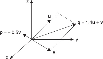
Figure 2.1 Linearly independent and dependent vectors
2.1.2 Basis, Norm and Inner Product
If ![]() is a basis for W, then any vector v ∈ W can be expressed uniquely as
is a basis for W, then any vector v ∈ W can be expressed uniquely as ![]() . If G′ is another basis of W, then G′ contains exactly the same number n of elements.
. If G′ is another basis of W, then G′ contains exactly the same number n of elements.
To quantify a measure of similarity or dissimilarity among vectors, we need to define the magnitude of a vector and the distance between vectors. We use the norm ||u|| of a vector u to define such a magnitude. In the area of topology, the metric is also used for defining a distance. To distinguish different vectors in a vector space, we define a measure of distance or metric between two vectors u and v as the norm ||u − v||. The norm must satisfy the following three rules.
Here, the notation ![]() stands for “for all” and iff stands for “if and only if”.
stands for “for all” and iff stands for “if and only if”.
2.1 

In addition to the distance between vectors, it is desirable to establish the concept of an angle between them. This requires the definition of an inner product.
In general, 〈u, v 〉 is a complex number, but 〈u, u 〉 is real. Note that 〈w, au + bv 〉 = ![]() 〈w, u 〉 +
〈w, u 〉 + ![]() 〈w, v 〉 and 〈u, 0 〉 = 0. If 〈u, v 〉 = 0 for all v ∈ V, then u = 0. Given any inner product,
〈w, v 〉 and 〈u, 0 〉 = 0. If 〈u, v 〉 = 0 for all v ∈ V, then u = 0. Given any inner product, ![]() is a norm on V.
is a norm on V.
For a real inner product space V, the inner product provides angle information between two vectors u and v. We denote the angle θ between u and v as
![]()
We interpret the angle as follows.
2.1.3 Hilbert Space
When we analyze a vector f in a vector space V having a basis ![]() , we wish to represent f as
, we wish to represent f as

Computation of the coefficients aj could be very laborious when the vector space V is not equipped with an inner product and ![]() is not an orthonomal set. A Hilbert space is a closed vector space equipped with an inner product.
is not an orthonomal set. A Hilbert space is a closed vector space equipped with an inner product.
For u, v, w ∈ H, a Hilbert space, we have the following properties.
- Cauchy–Schwarz inequality: |〈u, v 〉 | ≤ ||u|| ||v||.
- Triangle inequality: ||u + v|| ≤ ||u|| + ||v||.
- Parallelogram law: ||u + v||2 + ||u − v||2 = 2||u||2 + 2||v||2.
- Polarization identity: 4〈u, v 〉 = ||u + v||2 − ||u − v||2 + i||u + iv||2 − i||u − iv||2.
- Pythagorean theorem: ||u + v||2 = ||u||2 + ||v||2 if 〈u, v 〉 = 0.

Figure 2.2 Illustration of the Gram–Schmidt process

![]()
For the proof of the above theorem, see Rudin (1970). Let S be a closed subspace of a Hilbert space H. We define the orthogonal complement S⊥ of S as
![]()
According to the projection theorem, we can define a projection map PS:H → S such that the value PS(u) satisfies
![]()
This means that f(t) = ||u − PS(u) + tv||2 has its minimum at t = 0 for any v ∈ S and, therefore,
![]()
or
![]()
Hence, the projection theorem states that every u ∈ H can be uniquely decomposed as u = v + w with v ∈ S and w ∈ S⊥ and we can express the Hilbert space H as
![]()
From the Pythagorean theorem,
![]()
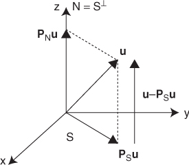
Figure 2.3 illustrate the projection of a vector u onto a subspace S.
Figure 2.3 Illustration of a projection of a vector u onto a subspace S

![]()


![]()
![]()

![]()
2.2 Vector Calculus
Based on the underlying physical principles, we need to express interrelations among system parameters, variables, excitations and measurements. A scalar-valued function f(x) defined in ![]() represents a numerical quantity at a point
represents a numerical quantity at a point ![]() . Examples may include temperature, voltage, pressure, altitude and so on. A vector-valued function F(x) is a vector quantity at
. Examples may include temperature, voltage, pressure, altitude and so on. A vector-valued function F(x) is a vector quantity at ![]() . It represents a vector field such as displacement, velocity, force, electric field intensity, magnetic flux density and so on. We now review the vector calculus of gradient, divergence and curl to handle basic dynamics among variables and parameters.
. It represents a vector field such as displacement, velocity, force, electric field intensity, magnetic flux density and so on. We now review the vector calculus of gradient, divergence and curl to handle basic dynamics among variables and parameters.
2.2.1 Gradient
Let ![]() . For a given unit vector
. For a given unit vector ![]() , the directional derivative of f at x in the direction b is denoted by ∂bf(x). It represents the rate of increase in f at x in the direction of b:
, the directional derivative of f at x in the direction b is denoted by ∂bf(x). It represents the rate of increase in f at x in the direction of b:
![]()
If b = ej, the jth unit vector in the Cartesian coordinate system, we simply write ![]() . The gradient of f, denoted as ∇f, is a vector-valued function that points in the direction of maximum increase of f:
. The gradient of f, denoted as ∇f, is a vector-valued function that points in the direction of maximum increase of f:
![]()
![]()
![]()
![]()
![]()
![]()
2.2.2 Divergence
The divergence of F(r) at a point r, written as div F, is the net outward flux of F per unit volume of a ball centered at r as the ball shrinks to zero:
![]()
where dS is the surface element, Br(r) is the ball with radius r and center r, and ∂B is the boundary of B, which is a sphere.
![]()
2.2.3 Curl
The circulation of a vector field F = (F1, F2, F3) around a closed path C in ![]() is defined as a scalar line integral of the vector F over the path C:
is defined as a scalar line integral of the vector F over the path C:
![]()
If F represents an electric field intensity, the circulation will be an electromotive force around the path C.
The curl of a vector field F, denoted by curl F, is a vector whose magnitude is the maximum net circulation of F per unit area as the area shrinks to zero and whose direction is the normal direction of the area when the area is oriented to make the net circulation maximum. We can define the b-directional net circulation of F at r precisely by
![]()
where ![]() is the disk centered at r with radius r and normal to d. Then, curl F is its maximum net circulation:
is the disk centered at r with radius r and normal to d. Then, curl F is its maximum net circulation:
![]()
![]()

2.2.4 Curve
A curve ![]() in
in ![]() and
and ![]() is represented, respectively, by
is represented, respectively, by
![]()
and
![]()
The curve ![]() is said to be regular if r′(t) ≠ 0 for all t. The arc length s(t) of
is said to be regular if r′(t) ≠ 0 for all t. The arc length s(t) of ![]() between r(t0) to r(t1) is given by
between r(t0) to r(t1) is given by
![]()
The unit tangent vector T of the curve ![]() is given by
is given by
![]()
The unit normal vector n of the curve ![]() is determined by
is determined by
![]()
where κ is the curvature given by
![]()
Here, we use |r′′ × r′| = |(s′)2κ T × (s′n)| = |(s′)3κ|. Note that dn/ds = − κ T since T · n = 0 and Ts · n + T · ns = 0.
2.2.5 Curvature
Consider a plane curve r(s) = (x(s), y(s)) in ![]() , where s is the length parameter. If θ(s) stands for the angle between T(s) and the x-axis, then κ(s) = dθ/ds because
, where s is the length parameter. If θ(s) stands for the angle between T(s) and the x-axis, then κ(s) = dθ/ds because
![]()
When the curve is represented as r(t) = (x(t), y(t)), then
![]()
Now, consider a curve ![]() given implicitly by the level set of
given implicitly by the level set of ![]() :
:
![]()
Then, the normal and tangent vectors to the level curve are
![]()
The curvature κ is
![]()
To see this, assume that ϕ(r(t)) = 0 and set y′ = − ϕx and x′ = ϕy because ∇ϕ(r) · r′(t) = 0. Then,
![]()
imply
![]()
Hence,
![]()
The curvature κ at a given point is the inverse of the radius of a disk that best fits the curve ![]() at that point.
at that point.
Next, we consider a space curve ![]() in
in ![]() represented by
represented by
![]()
Then
![]()
The curvature κ and torsion τ are computed by
![]()
where [ ] stands for the triple scalar product. If the relation between the moving coordinate system {T, N, B} and the fixed coordinates {x, y, z} is
![]()
then

We consider a regular surface ![]() :
:
![]()
Note that ![]() . The condition corresponding to the regularity of a space curve is that
. The condition corresponding to the regularity of a space curve is that
![]()
or

If |ru × rv| ≠ 0, the tangent vectors ru and rv generate a tangent plane that is spanned by ru and rv. The surface normal vector is expressed as
![]()
For example, if U = [0, 2π] × [0, π] and ![]() , then
, then ![]() represents the unit sphere. If the surface
represents the unit sphere. If the surface ![]() is written as z = f(x, y), then
is written as z = f(x, y), then
![]()
and the unit normal vector n is

If the surface ![]() is given by ϕ(r) = 0, then
is given by ϕ(r) = 0, then
![]()
2.3 Taylor's Expansion
The dynamics among system parameters, variables, excitations and measurements are often expressed as complicated nonlinear functions. In a nonlinear inverse problem, we may adopt a linearization approach in its solution-seeking process. Depending on the given problem, one may need to adopt a specific linearization process. In this section, we review Taylor's expansion as a tool to perform such an approximation.
Taylor polynomials are often used to approximate a complicated function. Taylor's expansion for ![]() about x is
about x is
2.2 ![]()
where O(|h|m+1) is the remainder term containing the (m + 1)th order of h. Precisely, the remainder term is
![]()
This expansion leads to numerical differential formulas of f in various ways, for example:
The Newton–Raphson method to find a root of f(x) = 0 can be explained from the first-order Taylor's approximation f(x + h) = f(x) + hf′(x) + O(h2) ignoring the term O(h2), which is negligible when h is small. The method is based on the approximation
![]()
It starts with an initial guess x0 and generates a sequence {xn} by the formula
![]()
It may not converge to a solution in general. The convergence issue will be discussed later.
We turn our attention to the second derivative f′′(x). By Taylor's expansion, we approximate f′′(x) by
![]()
The sign of f′′(x) gives local information about f for a sufficiently small positive h:
We consider a multi-dimensional case ![]() . The following fourth-order Taylor's theorem in n variables will be used later.
. The following fourth-order Taylor's theorem in n variables will be used later.


This leads to
![]()
If D2f(x) is a positive definite matrix, then, for a sufficiently small r,
![]()
which leads to the sub-MVP
![]()
Similarly, the super-MVP can be derived for a negative definite matrix D2f(x).
![]()

2.4 Linear System of Equations
We consider a linear system of equations including system parameters, variables, excitations and measurements. We may derive it directly from a linear physical system or through a linearization of a nonlinear system. Once we express a forward problem as a linear transform of inputs or system parameters to measured outputs, we can adopt numerous linear methods to seek solutions of the associated inverse problem. For the details of linear system of equations, please refer to Strang (2005, 2007).
2.4.1 Linear System and Transform
We consider a linear system in Figure 2.4. We express its outputs yi for i = 1, …, m as a linear system of equations:
2.3 
Using two vectors ![]() ,
, ![]() and a matrix
and a matrix ![]() , we can express the linear system as
, we can express the linear system as
or

Figure 2.4 Linear system with multiple inputs and multiple outputs

In most problems, the output vector y consists of measured data. If the input vector x includes external excitations or internal sources, the matrix ![]() is derived from the system transfer function or gain determined by the system structure and parameters. When the vector x contains system parameters, the linear system of equations in (2.4) is formulated subject to certain external excitations or internal sources, information about which is embedded in the matrix
is derived from the system transfer function or gain determined by the system structure and parameters. When the vector x contains system parameters, the linear system of equations in (2.4) is formulated subject to certain external excitations or internal sources, information about which is embedded in the matrix ![]() .
.
For the simplest case of m = n = 1, it is trivial to find x1 = y1/a11. If m = 1 and n > 1, that is, ![]() , it is not possible in general to determine all xj uniquely since they are summed to result in a single value y1. This requires us to increase the number of measurements so that m ≥ n. However, for certain cases, we will have to deal with the situation of m < n. Figure 2.5 illustrates three different cases of the linear system of equations. To obtain an optimal solution x by solving (2.4) for x, it is desirable to understand the structure of the matrix
, it is not possible in general to determine all xj uniquely since they are summed to result in a single value y1. This requires us to increase the number of measurements so that m ≥ n. However, for certain cases, we will have to deal with the situation of m < n. Figure 2.5 illustrates three different cases of the linear system of equations. To obtain an optimal solution x by solving (2.4) for x, it is desirable to understand the structure of the matrix ![]() in the context of vector spaces.
in the context of vector spaces.
Figure 2.5 Three cases of linear systems of equations

2.4.2 Vector Space of Matrix
We denote by ![]() a set of linear transforms from
a set of linear transforms from ![]() to
to ![]() , that is,
, that is, ![]() is the vector space consisting of m × n matrices
is the vector space consisting of m × n matrices

We call an m × 1 matrix a column vector and an 1 × n matrix a row vector. For the matrix A, we denote its ith row vector as
![]()
and its jth column vector as
![]()
For two vectors ![]() , we define their inner product by
, we define their inner product by
![]()
and define the outer product as

For ![]() and
and ![]() , we consider a linear transform or a linear system of equations:
, we consider a linear transform or a linear system of equations:
![]()
We can understand it as either
or
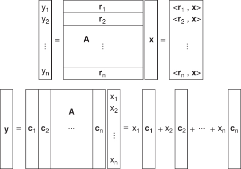
Figure 2.6 shows these two different representations of a linear system of equations ![]() for the case of m = n. In (2.5), each output yi is a weighted sum of all
for the case of m = n. In (2.5), each output yi is a weighted sum of all ![]() , and the row vector, row(A;i), provides weights for yi. In (2.6), the output vector y is expressed as a linear combination of n column vectors,
, and the row vector, row(A;i), provides weights for yi. In (2.6), the output vector y is expressed as a linear combination of n column vectors, ![]() with weights
with weights ![]() . It is very useful to have these two different views about the linear transform in (2.4) to better understand a solution of an inverse problem as well as the forward problem itself.
. It is very useful to have these two different views about the linear transform in (2.4) to better understand a solution of an inverse problem as well as the forward problem itself.
Figure 2.6 Two different representations of a linear system of equations y = Ax
We now summarize the null space, range and rank of a matrix ![]() before we describe how to solve
before we describe how to solve ![]() for x.
for x.
- The null space of a matrix
 is
is
![]()
- The range space of a matrix
 is
is
![]()
- The rank of a matrix
 , denoted by rank(A), is the maximum number of independent columns or rows.
2.7 ![]()
and
2.8 ![]()
If N(A) = {0}, the following are true:
If ![]() , the following hold:
, the following hold:
We also note that
![]()
2.4.3 Least-Squares Solution
We consider a linear system of equations y = Ax. If there are more equations than unknowns, that is, m > n, the system is over-determined and may not have any solution. On the other hand, if there are fewer equations than unknowns, that is, m < n, the system is under-determined and has infinitely many solutions. In these cases, we need to seek a best solution of y = Ax in an appropriate sense.
- x* is called the least − squares solution of y = Ax if
![]()
- x† is called the minimum−norm solution of y = Ax if x† is a least-squares solution of y = Ax and
![]()
If x* is the least-squares solution of y = Ax, then Ax* is the projection of y on R(A), and the orthogonality principle yields
![]()
If ATA is invertible, then
![]()
and the projection matrix on R(A) can be expressed as
2.9 ![]()
Since ||x||2 ≥ ||x†||2 for all x such that y = Ax,
![]()
that is, x† is orthogonal to N(A).
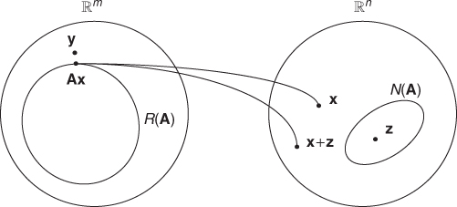
Figure 2.7 Least-squares and minimum-norm solutions of y = Ax
2.4.4 Singular Value Decomposition (SVD)
Let A be an m × n matrix. Then ATA can be decomposed into

where v1, …, vn are orthonormal eigenvectors of ATA. Since V is an orthogonal matrix, V−1 = VT.
If we choose ui = (1/σi)Avi, then
2.10 ![]()
and
2.11 ![]()
Since V−1 = VT, we have the singular value decomposition (SVD) of A:
2.12 ![]()
where

Suppose we number the ui, vi and σi so that σ1 ≥ σ2 ≥ ··· ≥ σr > 0 = σr+1 = ··· = σn. Then, we can express the singular value decomposition of A as
2.13 
This has the very useful property of splitting any matrix A into rank-one pieces ordered by their sizes:
2.14 ![]()
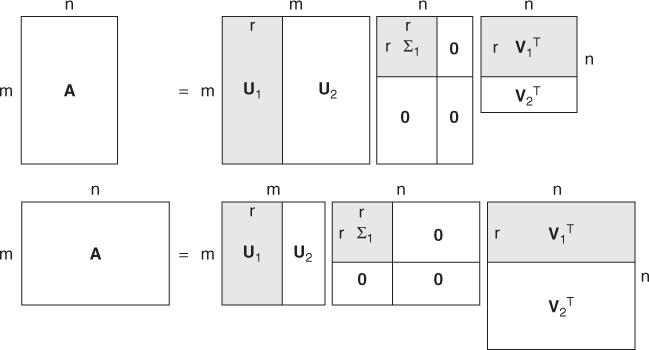
Figure 2.8 shows two graphical representations of the SVD. If σt+1, …, σr are negligibly small, we may approximate ![]() by the truncated SVD as
by the truncated SVD as
2.15 ![]()
with t < r.
Figure 2.8 Graphical representations of the SVD, ![]()
We may interpret the linear transform ![]() as shown in Figure 2.9. First, VTx provides coefficients of x along the input directions of
as shown in Figure 2.9. First, VTx provides coefficients of x along the input directions of ![]() . Second, ΣVTx scales VTx by
. Second, ΣVTx scales VTx by ![]() . Third, UΣVTx reconstructs the output y in the directions of
. Third, UΣVTx reconstructs the output y in the directions of ![]() . From the relation Avi = σiui, we can interpret v1 as the most sensitive input direction and u1 as the most sensitive output direction with the largest gain of σ1.
. From the relation Avi = σiui, we can interpret v1 as the most sensitive input direction and u1 as the most sensitive output direction with the largest gain of σ1.
Figure 2.9 Interpretation of ![]()

2.4.5 Pseudo-inverse
The pseudo-inverse of A is
2.16 ![]()
Here, in the pseudo-inverse Σ† of the diagonal matrix Σ, each σ ≠ 0 is replaced by 1/σ.
Since
2.17 ![]()
the products AA† and A†A can be viewed as projection matrices:
2.18 
We also know that A†y is in the row space of A = span{u1, …, ur} and Ax = y is solvable only when y is in the column space of A.
The least-squares solution x† = A†y minimizes
2.19 ![]()
Hence, x† satisfies the normal equation
2.20 ![]()
Moreover, x† is the smallest solution of ATAx = ATy because it has no null components.
2.5 Fourier Transform
Joseph Fourier (1768–1830) introduced the Fourier series to solve the heat equation. Since then, Fourier analysis has been widely used in many branches of science and engineering. It decomposes a general function f(x) into a linear combination of basic harmonics, sines or cosines, that is easier to analyze. For details of the theory, refer to Bracewell (1999) and Gasquet and Witomski (1998). We introduce the Fourier transform as a linear transform since it is also widely used in the inverse problem area.
2.5.1 Series Expansion
Assume that a set {ϕ0, ϕ1, …} is an orthonormal basis of a Hilbert space H, that is:
If we denote by Pn the projection map from H to Vn, then

If we denote ![]() , then
, then ![]() . By the Pythagorean theorem, we have
. By the Pythagorean theorem, we have
![]()
and we obtain the Bessel inequality
2.21 
By the Bessel inequality, the series

Moreover,
![]()
or
![]()
Hence,
![]()
This gives us the following series expansion:


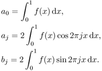


![]()

2.5.2 Fourier Transform
For each p with 1 ≤ p < ∞, we denote the class of measurable functions f on ![]() such that
such that ![]() by
by ![]() :
:
![]()
where the Lp-norm of f is
![]()
![]()
![]()
![]()
![]()
Let us summarize the Fourier transform pairs of some important functions.
- Scaling property:

- Shifting property:
![]()
- Dirac delta function:
![]()
- Dirac comb:
![]()
- Indicator function of the interval [a, b], denoted by χ[a, b](x), is
![]()
We have
![]()
- The Fourier transform of Gaussian function
 is given by

- The Fourier transform of f * g(x) = ∫f(x − y)g(y) dy is

- Modulation: if g(x) = f(x)cos(xi0x), then
![]()
- Derivative: if
 , then integrating by parts leads to
![]()
The following Fourier inversion provides that f can be recovered from its Fourier transform ![]() .
.
2.22 ![]()

![]()
![]()
Indeed, the Fourier inversion formula holds for general ![]() because
because ![]() is dense in
is dense in ![]() and
and ![]() . We omit the proof because it requires some time-consuming arguments of Lebesgue measure theory and some limiting process in L2. For a rigorous proof, please refer to Gasquet and Witomski (1998).
. We omit the proof because it requires some time-consuming arguments of Lebesgue measure theory and some limiting process in L2. For a rigorous proof, please refer to Gasquet and Witomski (1998).
The following Poisson summation formula indicates that the T-periodic summation of f is expressed as discrete samples of its Fourier transform ![]() with the sampling distance 1/T.
with the sampling distance 1/T.


![]()
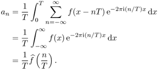
![]()

![]()
The band-limited function f with bandwidth B, that is, ![]() , does not contain sinusoidal waves at frequencies higher than B. This means that f cannot oscillate rapidly within a distance less than 1/(2B). Hence, the band-limited f can be represented by means of its uniformly spaced discrete sample {f(nΔx):n = 0, ± 1, ± 2, …} provided that the sampling interval Δx is sufficiently small. Indeed, the following sampling theorem states that, if Δx ≤ 1/(2B), then the discrete sample {f(nΔx):n = 0, ± 1, ± 2, …} contains the complete information about f. This 2B is called the Nyquist rate.
, does not contain sinusoidal waves at frequencies higher than B. This means that f cannot oscillate rapidly within a distance less than 1/(2B). Hence, the band-limited f can be represented by means of its uniformly spaced discrete sample {f(nΔx):n = 0, ± 1, ± 2, …} provided that the sampling interval Δx is sufficiently small. Indeed, the following sampling theorem states that, if Δx ≤ 1/(2B), then the discrete sample {f(nΔx):n = 0, ± 1, ± 2, …} contains the complete information about f. This 2B is called the Nyquist rate.
![]()


![]()
![]()
![]()
2.5.3 Discrete Fourier Transform (DFT)
Assume that f is a continuous signal such that
![]()
Choose a number N so that
![]()
With the condition N ≥ TΞ, the original signals f and ![]() are approximately recovered from the samples {f(kT/N − T/2):k = 0, 1, …, N − 1} and
are approximately recovered from the samples {f(kT/N − T/2):k = 0, 1, …, N − 1} and ![]() based on either the Poisson summation formula or the Whittaker–Shannon sampling theorem.
based on either the Poisson summation formula or the Whittaker–Shannon sampling theorem.
Let us convert the continuous signal f into the digital signal {f(kΔx − T/2):k = 0, 1, …, N − 1} with the sampling spacing Δx = T/N. The points xk = kΔx − T/2, with k = 0, 1, …, N − 1, are called the sampling points.
Writing fk = f(kΔx − T/2), the digital signal corresponding to the continuous signal f can be expressed in the following vector form:

Its Fourier transform ![]() for xi ∈ [ − Ξ/2, Ξ/2] is expressed approximately by
for xi ∈ [ − Ξ/2, Ξ/2] is expressed approximately by

Similarly, we denote ![]() where xij = jΔxi − Ξ/2 and Δxi = Ξ/N. Then, f(x) for x ∈ [ − T/2, T/2] is expressed approximately by
where xij = jΔxi − Ξ/2 and Δxi = Ξ/N. Then, f(x) for x ∈ [ − T/2, T/2] is expressed approximately by

In particular, we have

Since
![]()
we have the following approximations:

From the above approximations, we can define the discrete Fourier transform.
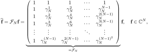
The DFT matrix ![]() has the following interesting properties.
has the following interesting properties.
- Let aj−1 be the jth row (or column) of the Fourier transform matrix
 . Then,
![]()
- The column vectors a0, …, aN−1 are eigenvectors of the following matrix corresponding to the Laplace operator:

- Hence, {a0, …, aN−1} forms an orthogonal basis over the N-dimensional vector space
 and
and

![]()
- If
 and
and  are the DFTs of f and g, then we have Parseval's identity:
![]()
2.5.4 Fast Fourier Transform (FFT)
The fast Fourier transform (FFT) is a DFT algorithm that reduces the number of computations from something on the order of N2 to NlogN. Let N = 2M and

From the definition of the DFT, we have

Since ![]() and
and ![]() , the (M + j, 2k)-component of the matrix
, the (M + j, 2k)-component of the matrix ![]() is
is
![]()
and the (M + j, 2k − 1)-component of the matrix ![]() is
is
![]()
The FFT is based on the following key identity:
2.26 
where ![]() is the N × N DFT matrix defined in the previous section and
is the N × N DFT matrix defined in the previous section and

![]()


2.5.5 Two-Dimensional Fourier Transform
The one-dimensional definition of the Fourier transform can be extended to higher dimensions. The Fourier transform of a two-dimensional function ρ(x, y), denoted by S(kx, ky), is defined by
![]()
We can generalize all the results in the one-dimensional Fourier transform to the two-dimensional case because the two-dimensional Fourier transform can be expressed as two one-dimensional Fourier transforms along x and y variables:

If ρ(x, y) and S(kx, ky) are a Fourier transform pair, we have the following properties.
- Scaling property:
![]()
- Shifting property:
![]()
- Modulation:
![]()
- Fourier inversion formula:
![]()
- Sampling theorem: if supp(S) ⊂ [ − B, B] × [ − B, B], then the original data ρ(x, y) can be reconstructed by the interpolation formula
![]()
References
Bracewell R 1999 The Fourier Transform and Its Applications, 3rd edn. McGraw-Hill, New York.
Gasquet C and Witomski P 1998 Fourier Analysis and Applications: Filtering, Numerical Computation, Wavelets. Springer, New York.
Rudin W 1970 Real and Complex Analysis. McGraw-Hill, New York.
Strang G 2005 Linear Algebra and Its Applications, 4th edn. Thomson Learning, London.
Strang G 2007 Computational Science and Engineering. Wellesley-Cambridge, Wellesley, MA.


