CHAPTER 9
Recursion
Recursion occurs when a method calls itself. The recursion can be direct (when the method calls itself) or indirect (when the method calls some other method that then calls the first method).
Recursion can also be single (when the method calls itself once) or multiple (when the method calls itself multiple times).
Recursive algorithms can be confusing because people don't naturally think recursively. For example, to paint a fence, you probably would start at one end and start painting until you reach the other. It is less intuitive to think about breaking the fence into left and right halves and then solving the problem by recursively painting each half.
However, some problems are naturally recursive. They have a structure that allows a recursive algorithm to easily keep track of its progress and find a solution. For example, a tree is recursive by nature, so algorithms that build, draw, and search trees are often recursive.
This chapter explains some useful algorithms that are naturally recursive. Some of these algorithms are useful by themselves, but learning how to use recursion in general is far more important than learning how to solve a single problem. Once you understand recursion, you can find it in many programming situations.
Recursion is not always the best solution, however, so this chapter also explains how you can remove recursion from a program when recursion might cause poor performance.
Basic Algorithms
Some problems have naturally recursive solutions. The following sections describe three naturally recursive algorithms that calculate factorials and Fibonacci numbers and solve the Tower of Hanoi problem.
These relatively straightforward algorithms demonstrate important concepts used by recursive algorithms. Once you understand them, you'll be ready to move on to the more complicated algorithms described in the following sections.
Factorial
The factorial of a number N is written N! and pronounced “N factorial.” You can define the factorial function recursively as follows:
![]()
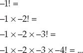
For example, the following equations show how you can use this definition to calculate 3!:
![]()
This definition leads to the following simple recursive algorithm:
Integer: Factorial(Integer: n) If (n == 0) Then Return 1 Return n * Factorial(n - 1) End Factorial
First, if the input value n equals 0, the algorithm returns 1. This corresponds to the first equation that defines the factorial function.
Otherwise, if the input is not 0, the algorithm returns the number n times the factorial of n - 1. This step corresponds to the second equation that defines the factorial function.
This is a very simple algorithm, but it demonstrates two important features that all recursive algorithms must have:
- Each time the method executes, it reduces the current problem to a smaller instance of the same problem and then calls itself to solve the smaller problem. In this example, the method reduces the problem of computing n! to the problem of computing (n - 1)! and then multiplying by n.
- The recursion must eventually stop. In this example, the input parameter n decreases with each recursive call until it equals 0. At that point, the algorithm returns 1 and does not call itself recursively, so the process stops.
Note that even this simple algorithm can create problems. If a program calls the Factorial method, passing it the parameter −1, the recursion never ends. Instead, the algorithm begins the following series of calculations:
One method that some programmers use to prevent this is to change the first statement in the algorithm to If (n <= 0) Then Return 1. Now if the algorithm is called with a negative parameter, it simply returns 1.
NOTE From a software engineering point of view, this may not be the best solution, because it hides a problem in the program that called the algorithm. It also returns the misleading value 1 when the true factorial of a negative number is undefined.
To detect problems in the calling code quickly, it may be better to explicitly check the value to make sure it is at least 0 and throw an exception if it is not.
Analyzing the run time performance of recursive algorithms is sometimes tricky, but it is easy for this particular algorithm. On input N, the Factorial algorithm calls itself N + 1 times to evaluate N!, (N − 1)!, (N − 2)!, ..., 0!. Each call to the algorithm does a small constant amount of work, so the total run time is O(N).
Because the algorithm calls itself N + 1 times, the maximum depth of recursion is also O(N). In some programming environments, the maximum possible depth of recursion may be limited, so this might cause a problem.
SERIOUS STACK SPACE
Normally a computer allocates two areas of memory for a program: the stack and the heap.
The stack is used to store information about method calls. When a piece of code calls a method, information about the call is placed on the stack. When the method returns, that information is popped off the stack, so the program can resume execution just after the point where it called the method. (The stack is the same kind of stack described in Chapter 5.) The list of methods that were called to get to a particular point of execution is called the call stack.
The heap is another piece of memory that the program can use to create variables and perform calculations.
Typically the stack is much smaller than the heap. The stack usually is large enough for normal programs because your code typically doesn't include methods calling other methods to a very great depth. However, recursive algorithms can sometimes create extremely deep call stacks and exhaust the stack space, causing the program to crash.
For this reason, it's important to evaluate the maximum depth of recursion that a recursive algorithm requires in addition to studying its run time and memory requirements.
However, the factorial function grows very quickly, so there's a practical limit to how big N can be in a normal program. For example, 20! ≈ 2.4 × 10¹⁸, and 21! is too big to fit in a 64-bit-long integer. If a program never calculates values larger than 20!, the depth of recursion can be only 20, and there should be no problem.
If you really need to calculate larger factorials, you can use other data types that can hold even larger values. For example, a 64-bit double-precision floating-point number can hold 170! ≈ 7.3 × 10306, and some data types, such as the .NET BigInteger type, can hold arbitrarily large numbers. In those cases, the maximum depth of recursion could be a problem. The section “Tail Recursion Removal” later in this chapter explains how you can prevent this kind of deep recursion from exhausting the stack space and crashing the program.
Fibonacci Numbers
The Fibonacci numbers are defined by these equations:
Fibonacci(0) = 0
Fibonacci(1) = 1
Fibonacci(n) = Fibonacci(n − 1) + Fibonacci(n − 2) for n > 1
For example, the first 12 Fibonacci numbers are 0, 1, 1, 2, 3, 5, 8, 13, 21, 34, 55, 89.
NOTE Some people define Fibonacci(0) = 1 and Fibonacci(1) = 1. This gives the same values as the definition shown here, just skipping the value 0.
The recursive definition leads to the following recursive algorithm:
Integer: Fibonacci(Integer: n) If (n <= 1) Then Return n Return Fibonacci(n - 1) + Fibonacci(n - 2); End Fibonacci
If the input n is 0 or 1, the algorithm returns 0 or 1. (If the input is 1 or less, the algorithm just returns the input.)
Otherwise, if the input is greater than 1, the algorithm calls itself for inputs n - 1 and n - 2, adds them together, and returns the result.
This recursive algorithm is reasonably easy to understand but is very slow. For example, to calculate Fibonacci(6) the program must calculate Fibonacci(5) and Fibonacci(4). But before it can calculate Fibonacci(5), the program must calculate Fibonacci(4) and Fibonacci(3). Here Fibonacci(4) is being calculated twice. As the recursion continues, the same values must be calculated many times. For large values of N, Fibonacci(N) calculates the same values an enormous number of times, making the program take a very long time.
Figure 9-1 shows the Fibonacci algorithm's call tree when it evaluates Fibonacci(6). Each node in the tree represents a call to the algorithm, with the indicated number as a parameter. The figure shows, for example, that the call to Fibonacci(6) in the top node calls Fibonacci(5) and Fibonacci(4). If you look at the figure, you can see that the tree is filled with duplicated calls. For example, Fibonacci(0) is calculated five times, and Fibonacci(1) is calculated eight times.
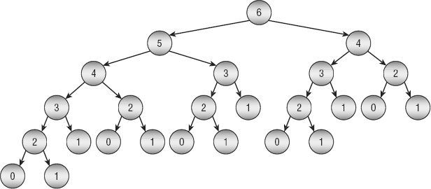
Figure 9-1: The Fibonacci algorithm's call tree is filled with duplicated calculations.
Analyzing this algorithm's run time is a bit trickier than analyzing the Factorial algorithm's run time, because this algorithm is multiply-recursive.
Suppose T(N) is the run time for the algorithm on input N. If N > 1, the algorithm calculates Fibonacci(N − 1) and Fibonacci(N − 2), performs an extra step to add those values, and returns the result. That means T(N) = T(N − 1) + T(N − 2) + 1.
This is slightly greater than T(N − 1) + T(N − 2). If you ignore the extra constant 1 at the end, this is the same as the definition of the Fibonacci function, so the algorithm has a run time at least as large as the function itself.
The Fibonacci function doesn't grow as quickly as the factorial function, but it still grows very quickly. For example, Fibonacci(92) ≈ 7.5x10¹⁸ and Fibonacci(93) doesn't fit in a long integer. That means you can calculate up to Fibonacci(92) with a maximum depth of recursion of 92, which shouldn't be a problem for most programming environments.
However, the run time of the Fibonacci algorithm grows very quickly. On my computer, calculating Fibonacci(44) takes more than a minute so calculating much larger values of the function is impractical anyway.
Tower of Hanoi
Chapter 5 introduced the Tower of Hanoi puzzle, in which a stack of disks, where each disk is smaller than the one below it, sits on one of three pegs. The goal is to transfer the disks from their starting peg to another peg by moving them one at a time and never placing a disk on top of a smaller disk. Figure 9-2 shows the puzzle from the side.
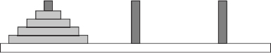
Figure 9-2: In the Tower of Hanoi puzzle, the goal is to move disks from one peg to another without placing a disk on top of a smaller disk.
Trying to solve the puzzle with a grand plan can be confusing, but there is a simple recursive solution. Instead of trying to think of solving the problem as a whole, you can reduce the problem size and then recursively solve the rest of the problem. The following pseudocode uses this approach to provide a simple recursive solution:
// Move the top n disks from peg from_peg to peg to_peg // using other_peg to hold disks temporarily as needed. TowerOfHanoi(Peg: from_peg, Peg: to_peg, Peg: other_peg, Integer: n) // Recursively move the top n - 1 disks from from_peg to other_peg. If (n > 1) Then TowerOfHanoi(from_peg, other_peg, to_peg, n - 1) // Move the last disk from from_peg to to_peg. <Move the top disk from from_peg to to_peg.> // Recursively move the top n - 1 disks back from other_peg to to_peg. If (n > 1) Then TowerOfHanoi(other_peg, to_peg, from_peg, n - 1) End TowerOfHanoi
The first step requires faith in the algorithm that seems to beg the question of how the algorithm works. That step moves the top n − 1 disks from the original peg to the peg that isn't the destination peg. It does this by recursively calling the TowerOfHanoi algorithm. At this point, how can you know that the algorithm works and can handle the smaller problem?
The answer is that the method recursively calls itself repeatedly if needed to move smaller and smaller stacks of disks. At some point in the sequence of recursive calls, the algorithm is called to move only a single disk. Then the algorithm doesn't call itself recursively. It simply moves the disk and returns.
The key is that each recursive call is used to solve a smaller problem. Eventually the problem size is so small that the algorithm can solve it without calling itself recursively.
As each recursive call returns, the algorithm's calling instance moves a single disk and then calls itself recursively again to move the smaller stack of disks to its final destination peg.
Figure 9-3 shows the series of high-level steps needed to move the stack from the first peg to the second. The first step recursively moves all but the bottom disk from the first peg to the third. The second step moves the bottom disk from the first peg to the second. The final step recursively moves the disks from the third peg to the second.
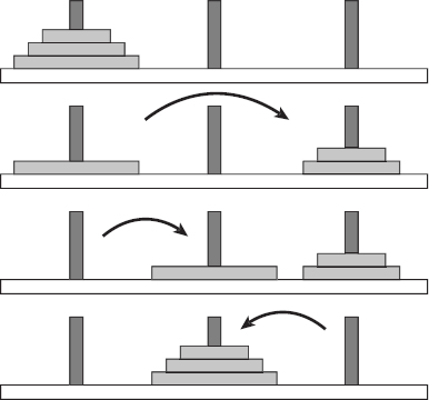
Figure 9-3: To move n disks, recursively move the upper n − 1 disks to the temporary peg. Then move the remaining disk to the destination peg. Finally, move the n − 1 upper disks from the temporary peg to the destination peg.
Figure 9-4 shows the entire sequence of moves needed to transfer a stack of three disks from the first peg to the second.
To analyze the algorithm's run time, let T(n) be the number of steps required to move n disks from one peg to another. Clearly T(1) = 1, because it takes one step to move a single disk from one peg to another.
For n > 0, T(n) = T(n − 1) + 1 + T(n − 1) = 2 × T(n − 1) + 1. If you ignore the extra constant 1, T(n) = 2 × T(n − 1) so the function has exponential run time O(2N).
To see this in another way, you can make a table similar to Table 9-1, giving the number of steps for various values of n. In the table, each value with n > 1 is calculated from the previous value by using the formula T(n) = 2 × T(n − 1) + 1. If you study the values, you'll see that T(n) = 2n− 1.
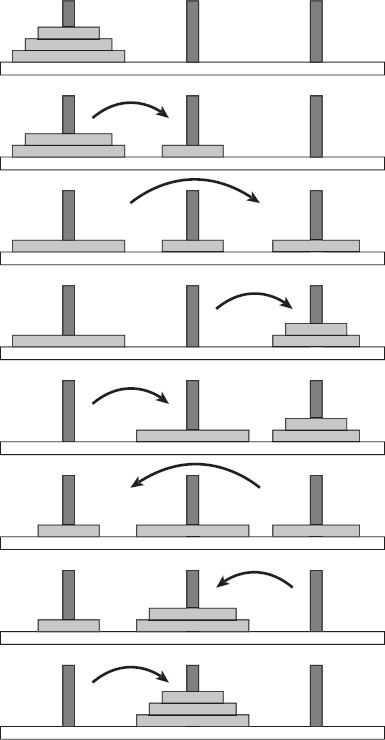
Figure 9-4: This sequence of steps transfers three disks from the first peg to the second.
Like the Fibonacci algorithm, the maximum depth of recursion for this algorithm on input N is N. Also like the Fibonacci algorithm, this algorithm's run time increases very quickly as N increases, so the run time limits the effective problem size long before the maximum depth of recursion does.
Table 9-1: Run Times for the Tower of Hanoi Puzzle
| n | T(n) |
| 1 | 1 |
| 2 | 3 |
| 3 | 7 |
| 4 | 15 |
| 5 | 31 |
| 6 | 63 |
| 7 | 127 |
| 8 | 255 |
| 9 | 511 |
| 10 | 1023 |
Graphical Algorithms
Several interesting graphical algorithms take advantage of recursion to produce intricate pictures with surprisingly little code. Although these algorithms are short, generally they are more confusing than the basic algorithms described in the preceding section.
Koch Curves
The Koch curve is good example of a particular kind of self-similar fractal, a curve in which pieces of the curve resemble the curve as a whole. These fractals start with an initiator, a curve that determines the fractal's basic shape. At each level of recursion, some or all of the initiator is replaced by a suitably scaled, rotated, and translated version of a curve called a generator. At the next level of recursion, pieces of the generator are then similarly replaced by new versions of the generator.
The simplest Koch curve uses a line segment as an initiator. Then, at each level of recursion, the segment is replaced with four segments that are one-third of the original segment's length. The first segment is in the direction of the original segment, the next is rotated −60 degrees, the third is rotated 120 degrees, and the final segment is in the original direction. Figure 9-5 shows this curve's initiator (left) and generator (right).
At the next level of recursion, the program takes each of the segments in the generator and replaces them with a new copy of the generator. Figure 9-6 shows the curve with levels of recursion 0 through 5.

Figure 9-5: This initiator (left) and generator (right) create the Koch curve.
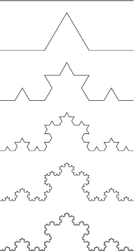
Figure 9-6: The Koch curve with levels of recursion 0 through 5 produces these shapes.
Looking at Figure 9-6, you can see why the curve is called self-similar. Parts of the curve look like smaller versions of the whole curve.
Let pt1, pt2, pt3, pt4, and pt5 be the points connected by the segments in the generator on the right in Figure 9-5. The following pseudocode shows how you might draw Koch curves:
// Draw a Koch curve with the given depth starting at point p1 // and going the distance "length" in the direction "angle." DrawKoch(Integer: depth, Point: pt1, Float: angle, Float: length) If (depth == 0) Then <Draw the line segment> Else <Find the points pt2, pt3, and pt4.> // Recursively draw the pieces of the curve. DrawKoch(depth - 1, pt1, angle, length / 3); DrawKoch(depth - 1, pt2, angle - 60, length / 3); DrawKoch(depth - 1, pt3, angle + 60, length / 3); DrawKoch(depth - 1, pt4, angle, length / 3); End If End DrawKoch
If depth is 0, the algorithm simply draws a line segment starting at point p1 going in direction angle for the distance length. (Exactly how you draw the segment depends on the programming environment you are using.)
If depth is greater than 0, the algorithm finds the points pt2, pt3, and pt4. It then draws a line segment starting at point pt1 going in direction angle for one-third of the original distance. From the new end point at pt2, it turns 60 degrees left and draws another segment one-third of the original distance. From the new end point at pt3 , it turns 120 degrees right (to an angle 60 degrees greater than the original angle) and draws another segment one-third of the original distance. Finally, from the last end point, pt4, the algorithm draws a segment at the original angle for one-third of the original distance.
If the depth is greater than 0, the algorithm calls itself recursively four times. If T(n) is the number of steps the algorithm uses for depth n, T(n) = 4 × T(n − 1) + C for some constant C. If you ignore the constant, T(n) = 4 × T(n − 1), so the algorithm has run time O(4N).
The maximum depth of recursion required to draw a depth N Koch curve is only N. Like the Fibonacci and Tower of Hanoi algorithms, this algorithm's run time grows so quickly that the maximum depth of recursion should never be a problem.
If you connect the edges of three Koch curves so that their initiators form a triangle, the result is called a Koch snowflake. Figure 9-7 shows a level 3 Koch snowflake.
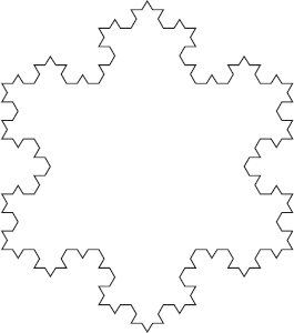
Figure 9-7: Three connected Koch curves form a Koch snowflake.
Hilbert Curve
Like the Koch curve, the Hilbert curve starts with a simple initiator curve. To move to a deeper level of recursion, the algorithm breaks the initiator into pieces and uses an appropriately rotated smaller version of the Hilbert curve to draw pieces of the initiator.
Figure 9-8 shows level 0, 1, and 2 Hilbert curves. In the level 1 and 2 curves, the lines connecting the lower-level curves are gray so that you can see how the pieces are connected to build the higher-level curves.
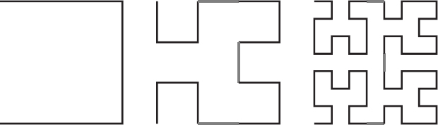
Figure 9-8: High-level Hilbert curves are made up of four connected lower-level curves.
The following pseudocode shows the Hilbert curve algorithm:
// Draw the Hilbert initially moving in the direction <dx, dy>. Hilbert(Integer: depth, Float: dx, Float: dy) If (depth > 0) Then Hilbert(depth - 1, dy, dx) DrawRelative(dx, dy) If (depth > 0) Then Hilbert(depth - 1, dx, dy) DrawRelative(dy, dx) If (depth > 0) Then Hilbert(depth - 1, dx, dy) DrawRelative(-dx, -dy) If (depth > 0) Then Hilbert(depth - 1, -dy, -dx) End Hilbert
The algorithm assumes that the program has defined a current drawing location. The DrawRelative method draws from that current position to a new point relative to that position and updates the current position. For example, if the current position is (10, 20), the statement DrawRelative(0, 10) would draw the line segment (10, 20) - (10, 30) and leave the new current position at (10, 30).
If the depth of recursion is greater than 0, the algorithm calls itself recursively to draw a version of the curve with one lower level of recursion and with the dx and dy parameters switched so that the smaller curve is rotated 90 degrees. If you compare the level 0 and level 1 curves shown in Figure 9-8, you can see that the level 0 curve that is drawn at the beginning of the level 1 curve is rotated.
Next the program draws a line segment to connect the first lower-level curve to the next one.
The algorithm then calls itself again to draw the next subcurve. This time it keeps dx and dy in their original positions so that the second subcurve is not rotated.
The algorithm draws another connecting line segment and then calls itself, again keeping dx and dy in their original positions so that the third subcurve is not rotated.
The algorithm draws another connecting line segment and then calls itself a final time. This time it replaces dx with -dy and dy with -dx so that the smaller curve is rotated −90 degrees.
Sierpi ski Curve
Like the Koch and Hilbert curves, the Sierpi![]() ski curve draws a higher-level curve by using lower-level copies of itself. Unlike the other curves, however, the simplest method of drawing a Sierpi
ski curve draws a higher-level curve by using lower-level copies of itself. Unlike the other curves, however, the simplest method of drawing a Sierpi![]() ski curve uses four indirectly recursive routines that call each other.
ski curve uses four indirectly recursive routines that call each other.
Figure 9-9 shows level 0, 1, 2, and 3 Sierpi![]() ski curves. In the level 1, 2, and 3 curves, the lines connecting the lower-level curves are gray so that you can see how the pieces are connected to build the higher-level curves.
ski curves. In the level 1, 2, and 3 curves, the lines connecting the lower-level curves are gray so that you can see how the pieces are connected to build the higher-level curves.
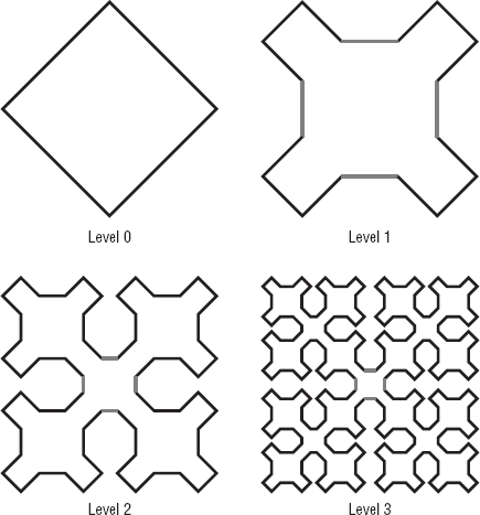
Figure 9-9: A Sierpi![]() ski curve is made up of four smaller Sierpi
ski curve is made up of four smaller Sierpi![]() ski curves.
ski curves.
Figure 9-10 shows the pieces of the level 1 Sierpi![]() ski curve. The curve consists of four sides that are drawn by four different routines and connected by line segments. The four routines draw curves that move the current drawing position in the right, down, left, and up directions. For example, the Right routine draws a series of segments that leaves the drawing position moved to the right. In Figure 9-10, the connecting line segments are drawn in gray.
ski curve. The curve consists of four sides that are drawn by four different routines and connected by line segments. The four routines draw curves that move the current drawing position in the right, down, left, and up directions. For example, the Right routine draws a series of segments that leaves the drawing position moved to the right. In Figure 9-10, the connecting line segments are drawn in gray.
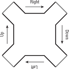
Figure 9-10: The level 1 Sierpi![]() ski curve is made up of pieces that go right, down, left, and up.
ski curve is made up of pieces that go right, down, left, and up.
To draw a higher-level version of one of the pieces of the curve, the algorithm breaks that piece into smaller pieces that have a lower level. For example, Figure 9-11 shows how you can make a depth 2 Right piece out of four depth 1 pieces. If you study Figure 9-9, you can figure out how to make the other pieces.

Figure 9-11: The level 2 Right piece is made up of pieces that go right, down, up, and right.
The following pseudocode shows the main algorithm:
// Draw a Sierpinski curve. Sierpinski(Integer: depth, Float: dx, Float: dy) SierpRight(depth, dx, dy) DrawRelative(dx, dy) SierpDown(depth, gr, dx, dy) DrawRelative(-dx, dy) SierpLeft(depth, dx, dy) DrawRelative(-dx, -dy) SierpUp(depth, dx, dy) DrawRelative(dx, -dy) End Sierpinski
The algorithm calls the methods SierpRight, SierpDown, SierpLeft, and SierpUp to draw the pieces of the curve. Between those calls, the algorithm calls DrawRelative to draw the line segments connecting the pieces of the curve. As was the case with the Hilbert curve, the DrawRelative method draws from that current position to a new point relative to that position and updates the current position. These calls to DrawRelative are the only places where the algorithm actually does any drawing.
The following pseudocode shows the SierpRight algorithm:
// Draw right across the top. SierpRight(Integer: depth, Float: dx, Float: dy) If (depth > 0) Then depth = depth - 1 SierpRight(depth, gr, dx, dy) DrawRelative(gr, dx, dy) SierpDown(depth, gr, dx, dy) DrawRelative(gr, 2 * dx, 0) SierpUp(depth, gr, dx, dy) DrawRelative(gr, dx, -dy) SierpRight(depth, gr, dx, dy) End If End SierpRight
You can follow this method's progress in Figure 9-11. First this method calls SierpRight to draw a piece of the curve moving to the right at a smaller depth of recursion. It then draws a segment down and to the right to connect to the next piece of the curve.
Next the method calls SierpDown to draw a piece of the curve moving downward at a smaller depth of recursion. It draws a segment to the right to connect to the next piece of the curve.
The method then calls SierpUp to draw a piece of the curve moving upward at a smaller depth of recursion. It draws a segment up and to the right to connect to the next piece of the curve.
The method finishes by calling SierpRight to draw a final piece of the curve moving to the right at a smaller depth of recursion.
Figuring out the other methods that draw pieces of the Sierpi![]() ski curve is left as an exercise.
ski curve is left as an exercise.
Space-filling curves such as the Hilbert and Sierpi![]() ski curves provide a simple method of approximate routing. Suppose you need to visit a group of stops in a city. If you draw a Hilbert or Sierpi
ski curves provide a simple method of approximate routing. Suppose you need to visit a group of stops in a city. If you draw a Hilbert or Sierpi![]() ski curve over the map of the city, you can visit the stops in the order in which they are visited by the curve. (You don't need to drive along the curve. You just use it to generate the ordering.)
ski curve over the map of the city, you can visit the stops in the order in which they are visited by the curve. (You don't need to drive along the curve. You just use it to generate the ordering.)
The result probably won't be optimal, but it probably will be reasonably good. You can use it as a starting point for the traveling salesperson problem (TSP) described in Chapter 17.
Because the Sierpi![]() ski methods call each other multiple times, they are multiply and indirectly recursive. Coming up with a nonrecursive solution from scratch would be difficult.
ski methods call each other multiple times, they are multiply and indirectly recursive. Coming up with a nonrecursive solution from scratch would be difficult.
Gaskets
A gasket is a type of self-similar fractal. To draw a gasket, you start with a geometric shape such as a triangle or square. If the desired depth of recursion is 0, you simply draw the shape. If the desired depth is greater than 0, the method subdivides the shape into smaller, similar shapes and then calls itself recursively to draw some but not all of them.
For example, Figure 9-12 shows depth 0 through 3 triangular gaskets that are often called Sierpi![]() ski gaskets (or Sierpi
ski gaskets (or Sierpi![]() ski sieves or Sierpi
ski sieves or Sierpi![]() ski triangles).
ski triangles).
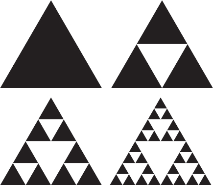
Figure 9-12: To create a Sierpi![]() ski gasket, divide a triangle into four pieces and recursively color the three at the triangle's corners.
ski gasket, divide a triangle into four pieces and recursively color the three at the triangle's corners.
Figure 9-13 shows a square gasket that is often called the Sierpi![]() ski carpet. (The Polish mathematician Wacław Franciszek Sierpi
ski carpet. (The Polish mathematician Wacław Franciszek Sierpi![]() ski, 1882–1969, studied lots of these sorts of shapes, so his name is attached to several.)
ski, 1882–1969, studied lots of these sorts of shapes, so his name is attached to several.)
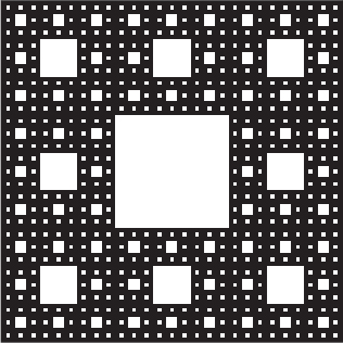
Figure 9-13: To create a Sierpi![]() ski carpet, divide a square into nine pieces, remove the center one, and recursively color the rest.
ski carpet, divide a square into nine pieces, remove the center one, and recursively color the rest.
Writing low-level pseudocode to draw the Sierpi![]() ski gasket and carpet is left as an exercise.
ski gasket and carpet is left as an exercise.
Backtracking Algorithms
Backtracking algorithms use recursion to search for the best solution to complicated problems. These algorithms recursively build partial test solutions to solve the problem. When they find that a test solution cannot lead to a usable final solution, they backtrack, discarding that test solution and continuing the search from farther up the call stack.
Backtracking is useful when you can incrementally build partial solutions and you can sometimes quickly determine that a partial solution cannot lead to a complete solution. In that case, you can stop improving that partial solution, backtrack to the previous partial solution, and continue the search from there.
The following pseudocode shows the general backtracking approach at a high level:
// Explore this test solution. // Return false if it cannot be extended to a full solution. // Return true if a recursive call to LeadsToSolution finds // a full solution. Boolean: LeadsToSolution(Solution: test_solution) // If we can already tell that this partial solution cannot // lead to a full solution, return false. If <test_solution cannot solve the problem> Then Return false // If this is a full solution, return true. If <test_solution is a full solution> Then Return true // Extend the partial solution. Loop <over all possible extensions to test_solution> <Extend test_solution> // Recursively see if this leads to a solution. If (LeadsToSolution(test_solution)) Then Return true // This extension did not lead to a solution. Undo the change. <Undo the extension> End Loop // If we get here, this partial solution cannot // lead to a full solution. Return false End LeadsToSolution
The LeadsToSolution algorithm takes as a parameter whatever data it needs to keep track of a partial solution. It returns true if that partial solution leads to a full solution.
The algorithm begins by testing the partial solution to see if it is illegal. If the test solution so far cannot lead to a feasible solution, the algorithm returns false. The calling instance of LeadsToSolution abandons this test solution and works on others.
If the test solution looks valid so far, the algorithm loops over all the possible ways it can extend the solution toward a full solution. For each extension, the algorithm calls itself recursively to see if the extended solution will work. If the recursive call returns false, that extension doesn't work, so the algorithm undoes the extension and tries again with a new extension.
If the algorithm tries all possible extensions to the test solution and cannot find a feasible solution, it returns false so that the calling instance of LeadsToSolution can abandon this test solution.
You can think of the quest for a solution as a search through a hypothetical decision tree. Each branch in the tree corresponds to a particular decision attempting to solve the problem. For example, an optimal chess game tree would contain branches for every possible move at a given point in the game. If you can use a relatively quick test to realize that a partial solution cannot produce a solution, you can trim the corresponding branch off the tree without searching it exhaustively. That can remove huge chunks from the tree and save a lot of time. (The idea of decision trees is described further in Chapter 12.)
The following sections describe two problems that have natural backtracking algorithms: the eight queens problem and the knight's tour problem. When you study the algorithms for those problems, the more general solution shown here should be easier to understand.
Eight Queens Problem
In the eight queens problem, the goal is to position eight queens on a chessboard so that none of them can attack any of the other queens. In other words, no two queens can be in the same row, column, or diagonal. Figure 9-14 shows one solution to the eight queens problem.
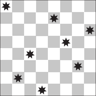
Figure 9-14: In the eight queens problem, you must position eight queens on a chessboard so that none can attack any of the others.
One way to solve this problem would be to try every possible arrangement of eight queens on a chessboard. Unfortunately, ![]() = 4,426,165,368 arrangements are possible. You could enumerate all of them, but doing so would be time-consuming.
= 4,426,165,368 arrangements are possible. You could enumerate all of them, but doing so would be time-consuming.
The reason there are so many possible arrangements of queens is that you can position 8 queens in any of 64 squares. The queens are identical so it doesn't matter which queen you use in a given location. That means the number of possible arrangements is the same as the number of ways you can pick 8 squares out of the possible 64.
The number of selections of k items from a set of n without duplicates is given by the binomial coefficient. That value is written ![]() and is pronounced “n choose k.” You can calculate the value with this formula:
and is pronounced “n choose k.” You can calculate the value with this formula:
![]()
For example, this equation gives the number of different selections of three items from a set of five without duplicates:
![]()
The number of selections of k items from a set of n allowing duplicates (if you are allowed to pick the same item more than once in a selection) is given by this formula:
![]()
For example, this equation gives the number of different selections of three items from a set of five allowing duplicates:
![]()
In the eight queens, you need to find the number of ways to pick 8 of the squares without duplicates (you can't put more than one queen on the same square). The number of possible selections is:
![]()
Backtracking works well for this problem because it allows you to eliminate certain possibilities from consideration. For example, you could start with a partial solution that places a queen on the board's upper-left corner. You might try adding another queen just to the right of the first queen, but you know that placing two queens on the same row isn't allowed. This means you can eliminate every possible solution that has the first two queens next to each other in the upper-left corner. The program can backtrack to the point before it added the second queen and search for more promising solutions.
This may seem like a trivial benefit. After all, you know a solution cannot have two queens side by side in the upper-left corner. However, ![]() = 61,474,519 possible arrangements of eight queens on a chessboard have queens in those positions, so one backtracking step saves you the effort of examining more than 61 million possibilities.
= 61,474,519 possible arrangements of eight queens on a chessboard have queens in those positions, so one backtracking step saves you the effort of examining more than 61 million possibilities.
In fact, if the first queen is placed in the upper-left corner, no other queen can be placed in the same row, column, or diagonal. That means there are a total of 21 places where the second queen cannot be placed. Eliminating all those partial solutions removes almost 1.3 billion possible arrangements from consideration.
Later tests remove other partial solutions from consideration. For example, after you place the second queen somewhere legal, it restricts where the third queen can be placed further.
The following pseudocode shows how you can use backtracking to solve the eight queens problem:
Boolean: EightQueens(Boolean: spot_taken[,], Integer: num_queens_positioned) // See If the test solution is already illegal. If (Not IsLegal(spot_taken)) Then Return false // See if we have positioned all of the queens. If (num_queens_positioned == 8) Then Return true // Extend the partial solution. // Try all positions for the next queen. For row = 0 to 7 For col = 0 to 7 // See if this spot is already taken. If (Not spot_taken[row, col]) Then // Put a queen here. spot_taken[row, col] = true // Recursively see if this leads to a solution. If (EightQueens(spot_taken, num_queens_positioned + 1)) Then Return true // The extension did not lead to a solution. // Undo the change. spot_taken[row, col] = false End If Next col Next row // If we get here, we could not find a valid solution. Return false End EightQueens
The algorithm takes as a parameter a two-dimensional array of booleans named spot_taken. The entry spot_taken[row, col] is true if there is a queen in row row and column col.
The algorithm's second parameter, num_queens_positioned, specifies how many queens have been placed in the test solution.
The algorithm starts by calling IsLegal to see if the test solution so far is legal. The IsLegal method, which isn't shown here, simply loops through the spot_taken array to see if there are two queens in the same row, column, or diagonal.
Next the algorithm compares num_queens_positioned with the total number of queens, 8. If all the queens have been positioned, this test solution is a full solution, so the algorithm returns true. (The spot_taken array is not modified after that point, so when the first call to EightQueens returns, the array holds the solution.)
If this is not a full solution, the algorithm loops over all the rows and columns. For each row/column pair, it checks spot_taken to see if that spot already contains a queen. If the spot doesn't hold a queen, the algorithm puts the next queen there and calls itself recursively to see if the extended solution leads to a full solution.
If the recursive call returns true, it found a full solution, so this call also returns true.
If the recursive call returns false, the extended solution does not lead to a solution, so the algorithm removes the queen from its new position and tries the next possible position.
If the algorithm tries all possible locations for the next queen and none of them works, this test solution (before the new queen is added) cannot lead to a full solution, so the algorithm returns false.
You can improve this algorithm's performance in a couple of interesting ways. See Exercises 13 and 14 for details.
Knight's Tour
In the knight's tour problem, the goal is to make a knight visit every position on a chessboard without visiting any square twice. A tour is considered closed if the final position is one move away from the starting position, and the knight could immediately start the tour again. A tour that is not closed is considered open.
NOTE In case you don't remember, a knight moves two squares horizontally or vertically and then one square perpendicularly from its current position, as shown in Figure 9-15.
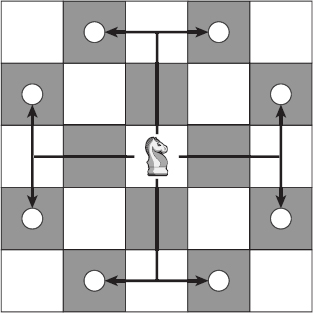
Figure 9-15: In chess, a knight can move to eight places if none of them lies off the board.
The following pseudocode shows a backtracking solution to the knight's tour problem:
// Move the knight to position [row, col]. Then recursively try // to make other moves. Return true if we find a valid solution. Boolean: KnightsTour(Integer: row, Integer: col) Integer: move_number[,], Integer: num_moves_taken) // Move the knight to this position. num_moves_taken = num_moves_taken + 1 move_number[row, col] = num_moves_taken // See if we have made all the required moves. If (num_moves_taken == 64) Then Return true // Build arrays to determine where legal moves are // with respect to this position. Integer: dRows[] = { −2, −2, −1, 1, 2, 2, 1, −1 } Integer: dCols[] = { −1, 1, 2, 2, 1, −1, −2, −2 } // Try all legal positions for the next move. For i = 0 To 7 Integer: r = row + d_rows[i] Integer: c = col + d_cols[i] If ((r >= 0) And (r < NumRows) And (c >= 0) And (c < NumCols) And (move_number[r, c] == 0)) Then // This move is legal and available. Make this move // and then recursively try other assignments. If (KnightsTour(r, c, move_number, num_moves_taken) Then Return true End If Next i // This move didn't work out. Undo it. move_number[row, col] = 0 // If we get here, we did not find a valid solution. return false End KnightsTour
This algorithm takes as parameters the row and column where the knight should move next, an array named move_number that gives the number of the move when the knight visited each square, and the number of moves made so far.
The algorithm starts by recording the knight's move to the current square and incrementing the number of moves made. If the number of moves made is 64, the knight has finished a tour of the board, so the algorithm returns true to indicate success.
If the tour is not finished, the algorithm initializes two arrays to represent the moves that are possible from the current square. For example, the first entries in the arrays are −2 and −1, indicating that the knight can move from square (row, col) to (row - 2, col - 1) if that square is on the board.
Next the algorithm loops through all the possible moves from the position (row, col). If a move is on the board and has not already been visited in the test tour, the algorithm makes the move and recursively calls itself to see if that leads to a full solution.
If none of the possible moves from the current position leads to a solution, the algorithm sets move_number[row, col] = 0 to undo the current move and returns false to indicate that moving the knight to square (row, col) does not lead to a solution.
Unfortunately, the knight's tour problem isn't as easy to constrain as the eight queens problem. With the eight queens problem, it's fairly easy to tell whether a new position is under attack by another queen and therefore unavailable for a new queen. In that case you can eliminate that position from consideration.
In the knight's tour, any position the knight can reach that has not yet been visited gives a new test solution. There may be some cases where you can easily conclude that a test solution won't work, such as if the board has an unvisited square that is more than one move away from any other unvisited square, but recognizing that situation is difficult.
The fact that it's hard to eliminate test solutions early on means the algorithm often follows a test solution for a long while before discovering that the solution is infeasible. A knight can have up to eight legal moves, so an upper bound on the number of potential tours is 864, or roughly 6.3 × 1057. You can study the positions on the board to get a better estimate of the potential number of tours (for example, a knight in a corner has only two possible moves), but the total number of potential tours is an enormous number in any case.
All this means it's difficult to solve the knight's tour problem for a normal 8 × 8 chessboard. In one set of tests, a program solved the problem on a 6 × 6 board almost instantly and on a 7 × 6 board in about 2 seconds. It still hadn't found a solution on a 7 × 7 board after an hour.
Although solving the knight's tour using only backtracking is difficult, a heuristic solves the problem quite well. A heuristic is an algorithm that often produces a good result but that is not guaranteed to produce the best possible result. For example, a driving heuristic might be to add 10 percent more time to expected travel time to allow for traffic delays. Doing so doesn't guarantee that you'll always be on time, but it increases the chances.
In 1823 H. C. von Warnsdorff suggested a knight's tour heuristic in which at each step the algorithm should select the next possible move that has the lowest number of possible moves leading out of it.
For example, suppose the knight is in a position where it has only two possible moves. If the knight makes the first move, it then has five possible locations for its next move. If the knight makes the second move, it has only one possible move for its next move. In that case, the heuristic says the algorithm should try the second move first.
This heuristic is so good that it finds a complete tour with no backtracking for boards of size up to 75 × 75. (In my test, the program found a solution on a 57 × 57 board almost instantly and then crashed with a stack overflow on a 58 × 58 board.)
Selections and Permutations
A selection or combination is a subset of a set of objects. For example, in the set {A, B, C}, the subset {A, B} is a selection. All the selections for the set {A, B, C} are {A, B}, {A, C}, and {B, C}. In a section, the ordering of the items in a set doesn't matter so {A, B} is considered the same as {B, A}.
You can think of this as being similar to a menu selection at a restaurant. Selecting a cheese sandwich and milk is the same as selecting milk and a cheese sandwich.
A permutation is an ordered arrangement of a subset of items taken from a set. This is similar to a selection, except that the ordering matters. For example, (A, B) and (B, A) are two permutations of two items taken from the set {A, B, C}. All the permutations of two items taken from the set {A, B, C} are (A, B), (A, C), (B, A), (B, C), (C, A), and (C, B). (Notice the notation uses brackets { } for unordered selections and parentheses ( ) for ordered permutations.)
One other factor determines which groups of items are included in a particular kind of selection or permutation: whether duplicates are allowed. For example, the two-item selections for the set {A, B, C} allowing duplicates include {A, A}, {B, B}, and {C, C} in addition to the other selections listed earlier.
The special case of a permutation that takes all the items in the set and doesn't allow duplicates gives all the possible arrangements of the items. For the set {A, B, C}, all the arrangements are (A, B, C), (A, C, B), (B, A, C), (B, C, A), (C, A, B), and (C, B, A). Many people think of the permutations of a set to be this collection of arrangements, rather than the more general case, in which you may not be taking all the items from the set and you may allow duplicates.
The following sections describe algorithms you can use to generate selections and permutations with and without duplicates:
Selections with Loops
If you know how many items you want to select from a set when you are writing a program, you can use a series of For loops to easily generate combinations. For example, the following pseudocode generates all the selections of three items taken from a set of five items allowing duplicates:
// Generate selections of 3 items allowing duplicates. List<string>: Select3WithDuplicates(List<string> items) List<string>: results = New List<string> For i = 0 To <Maximum index in items> For j = i To <Maximum index in items> For k = j To <Maximum index in items> results.Add(items[i] + items[j] + items[k]) Next k Next j Next i Return results End Select3WithDuplicates
This algorithm takes as a parameter a list of Strings. It then uses three For loops to select the three letters that make up each selection.
Each loop starts with the current value of the previous loop's counter. For example, the second loop starts with j equal to i. That means the second letter chosen for the selection will not be a letter that comes before the first letter in the items. For example, if the items include the letters A, B, C, D, and E, and the first letter in the selection is C, the second letter won't be A or B. That keeps the letters in the selection in alphabetical order and prevents the algorithm from selecting both {A, B, C} and {A, C, B}, which are the same set.
Within the innermost loop, the algorithm combines the items selected by each loop variable to produce an output that includes all three selections.
Modifying this algorithm to prevent duplicates is simple. Just start each loop at the value 1 greater than the current value in the next outer loop. The following pseudocode shows this modification:
// Generate selections of 3 items without allowing duplicates. List<string>: Select3WithoutDuplicates(List<string> items) List<string>: results = new List<string>() For i = 0 To <Maximum index in items> For j = i + 1 To <Maximum index in items> For k = j + 1 To <Maximum index in items> results.Add(items[i] + items[j] + items[k]) Next k Next j Next i Return results End Select3WithoutDuplicates
This time each loop starts at 1 greater than the previous loop's current value, so a loop cannot select the same item as a previous loop, and that prevents duplicates.
The sidebar “Counting Combinations” earlier in this chapter explains how you can calculate the number of possible selections for a given set and number of items to select.
Selections with Duplicates
The problem with the algorithms described in the preceding section is that they require you to know how many items you will select when you write the code, and sometimes that may not be the case. If you don't know how many items are in the original set of items, the program can figure that out. However, if you don't know how many items to select, you can't program the right number of For loops.
You can solve this problem recursively. Each recursive call to the algorithm is responsible for adding a single selection to the result. Then, if the result doesn't include enough selections, the algorithm calls itself recursively to make more. When the selection is complete, the algorithm does something with it, such as printing the list of items selected.
The following pseudocode shows a recursive algorithm that generates selections allowing duplicates:
// Generate combinations allowing duplicates. SelectKofNwithDuplicates(Integer: index, Integer: selections[], Data: items[], List<List<Data>> results) // See if we have made the last assignment. If (index == <Length of selections>) Then // Add the result to the result list. List<Data> result = New List<Data>() For i = 0 To <Largest index in selections> result.Add(items[selections[i]]) Next i results.Add(result) Else // Get the smallest value we can use for the next selection. Integer: start = 0 // Use this value if this is the first index. If (index > 0) Then start = selections[index - 1] // Make the next assignment. For i = start To <Largest index in items> // Add item i to the selection. selections[index] = i // Recursively make the other selections. SelectKofNwithDuplicates(index + 1, selections, items, results) Next i End If End SelectKofNwithDuplicates
This algorithm takes the following parameters:
- index gives the index of the item in the selection that this recursive call to the algorithm should set. If index is 2, this call to the algorithm fills in selections[2].
- selections is an array to hold the indices of the items in a selection. For example, if selections holds two entries and its values are 2 and 3, the selection includes the items with indices 2 and 3.
- items is an array of the items from which selections should be made.
- results is a list of lists of items representing the complete selections. For example, if a selection is {A, B, D}, results holds a list including the indices of A, B, and D.
When the algorithm starts, it checks the index of the item in the selection it should make. If this value is greater than the length of the selections array, the selection is complete, so the algorithm adds it to the results list.
If the selection is incomplete, the algorithm determines the smallest index in the items array that it could use for the next choice in the selection. If this call to the algorithm is filling in the first position in the selections array, it could use any value in the items array, so start is set to 0. If this call does not set the first item in the selection, the algorithm sets start to the index of the last value chosen.
For example, suppose the items are {A, B, C, D, E} and the algorithm has been called to fill in the third choice. Suppose also that the first two choices were the items with indices 0 and 2, so the current selection is {A, C}. In that case the algorithm sets start to 3, so the items it considers for the next position have indices of 3 or greater. That makes it pick between D and E for this selection.
Setting start in this way keeps the items in the selection in order. In this example, that means the letters in the selection are always in alphabetical order. That prevents the algorithm from picking two selections such as {A, C, D} and {A, D, C}, which are the same items in a different order.
Having set start, the algorithm loops from start to the last index in the items array. For each of those values, the algorithm places the value in the selections array to add the corresponding item to the selection and then calls itself recursively to assign values to the other entries in the selections array.
Selections Without Duplicates
To produce selections without duplicates, you need to make only one minor change to the previous algorithm. Instead of setting the start variable equal to the index last added to the selections array, set it to 1 greater than that index. That prevents the algorithm from selecting the same value again.
The following pseudocode shows the new algorithm with the modified line highlighted:
// Generate combinations allowing duplicates. SelectKofNwithoutDuplicates(Integer: index, Integer: selections[], Data: items[], List<List<Data>> results) // See if we have made the last assignment. If (index == <Length of selections>) Then // Add the result to the result list. List<Data> result = New List<Data>() For i = 0 To <Largest index in selections> Result.Add(items[selections[i]]) Next i results.Add(result) Else // Get the smallest value we can use for the next selection. Integer: start = 0 // Use this value if this is the first index. If (index > 0) Then start = selections[index - 1] + 1 // Make the next assignment. For i = start To <Largest index in items> // Add item i to the selection. selections[index] = i // Recursively make the other selections. SelectKofNwithoutDuplicates( index + 1, selections, items, results) Next i End If End SelectKofNwithoutDuplicates
The algorithm works the same way as before, but this time each choice for an item in the selection must come after the one before it in the items list. For example, suppose the items are {A, B, C, D}, the algorithm has already chosen {A, B} for the partial selection, and now the algorithm has been called to make the third selection. In that case, the algorithm considers only the items that come after B, which are C and D.
Permutations with Duplicates
The algorithm for generating permutations is very similar to the previous ones for generating selections. The following pseudocode shows the algorithm for generating permutations allowing duplicates:
// Generate permutations allowing duplicates. PermuteKofNwithDuplicates(Integer: index, Integer: selections[] Data: items[], List<List<Data>> results // See if we have made the last assignment. If (index == <Length of selections>) Then // Add the result to the result list. List<Data> result = New List<Data>() For i = 0 To <Largest index in selections> Result.Add(items[selections[i]] Next i results.Add(result Else // Make the next assignment. For i = 0 To <Largest index in items> // Add item i to the selection. selections[index] = i // Recursively make the other assignments. PermuteKofNwithDuplicates(index + 1, selections, items, results) Next i End If End PermuteKofNwithDuplicates
The main difference between this algorithm and the earlier one for generating selections with duplicates is that this algorithm loops through all the items when it makes its assignment instead of starting the loop at a start value. This allows the algorithm to pick items in any order, so it generates all the permutations.
COUNTING PERMUTATIONS WITH DUPLICATES
Suppose you're making permutations of k out of n items allowing duplicates. For each item in a permutation, the algorithm could pick any of the n choices. It makes k independent choices (in other words, one choice does not depend on the previous choices), so there are n * n * ... * n = nk possible permutations.
In the special case where you want to generate permutations that select all n of the n items, nn results are possible.
Just as you can define selections without duplicates, you can define permutations without duplicates.
Permutations Without Duplicates
To produce permutations without duplicates, you need to make only one minor change to the preceding algorithm. Instead of allowing all the items to be selected for each assignment, the algorithm excludes any items that have already been used.
The following pseudocode shows the new algorithm with the modified lines highlighted:
// Generate permutations not allowing duplicates. PermuteKofNwithoutDuplicates(Integer: index, Integer: selections[], Data: items[], List<List<Data>> results) // See if we have made the last assignment. If (index == <Length of selections>) Then // Add the result to the result list. List<Data> result = New List<Data>() For i = 0 To <Largest index in selections> Result.Add(items[selections[i]]) Next i results.Add(result) Else // Make the next assignment. For i = 0 To <Largest index in items> // Make sure item i hasn't been used yet. Boolean: used = false For j = 0 To index - 1 If (selections[j] == i) Then used = true Next j If (Not used) Then // Add item i to the selection. selections[index] = i // Recursively make the other assignments. PermuteKofNwithoutDuplicates( index + 1, selections, items, results) End If Next i End If End PermuteKofNwithoutDuplicates
The only change is that this version of the algorithm checks that an item has not been used yet in a permutation before adding it.
COUNTING PERMUTATIONS WITHOUT DUPLICATES
Suppose you're making permutations of k out of n items without duplicates. For the first item in a permutation, the algorithm could pick any of the n choices. For the second item, it could pick any of the remaining n − 1 items. Multiplying the number of choices at each step gives the total number of possible permutations: n × (n − 1) × (n − 2) × ... × (n − k + 1).
In the special case where k = n, so that you are generating permutations that select all n of the items without duplicates, this formula becomes n × (n − 1) × (n − 2) × ... 1 = n! This is the number most people think of as the number of permutations of a set.
Most people think of permutations as being the permutations of n out of the n objects without duplicates.
Recursion Removal
Recursion makes some problems easier to understand. For example, the recursive solution to the Tower of Hanoi problem is simple and elegant.
Unfortunately, recursion has some drawbacks. Sometimes it leads to solutions that are natural but inefficient. For example, the recursive algorithm for generating Fibonacci numbers requires that the program calculate the same values many times. This slows it down so much that calculating more than the 50th or so value is impractical.
Other recursive algorithms cause a deep series of calls, and that can make the program exhaust its call stack. The knight's tour with Warnsdorff's heuristic demonstrates that problem. The heuristic can solve the knight's tour problem for boards up to 57 × 57 on my computer, but beyond that it exhausts the call stack.
Fortunately, you can do a few things to address these problems. The following sections describe some approaches you can take to restructure or remove recursion to improve performance.
Tail Recursion Removal
Tail recursion occurs when the last thing a singly recursive algorithm does before returning is call itself. For example, consider the following implementation of the Factorial algorithm:
Integer: Factorial(Integer: n) If (n == 0) Then Return 1 Integer: result = n * Factorial(n - 1) Return result End Factorial
The algorithm starts by checking to see if it needs to call itself recursively or if it can simply return the value 1. If the algorithm must call itself, it does so, multiplies the returned result by n, and returns the result.
You can convert this recursive version of the algorithm into a nonrecursive version by using a loop. Within the loop, the algorithm performs whatever tasks the original algorithm did.
Before the end of the loop, the algorithm should set its parameters to the values they had during the recursive call. If the algorithm returns a value, as the Factorial algorithm does, you need to create a variable to keep track of the return value.
When the loop repeats, the parameters are set for the recursive call, so the algorithm does whatever the recursive call did.
The loop should end when the condition occurs that originally ended the recursion.
For the Factorial algorithm, the stopping condition is n == 0, so that condition controls the loop.
When the algorithm calls itself recursively, it decreases its parameter n by 1, so the non-recursive version should also decrease n by 1 before the end of the loop.
The following pseudocode shows the new nonrecursive version of the Factorial algorithm:
Integer: Factorial(Integer: n) // Make a variable to keep track of the returned value. // Initialize it to 1 so we can multiply it by returned results. // (The result is 1 if we do not enter the loop at all.) Integer: result = 1 // Start a loop controlled by the recursion stopping condition. While (n != 0) // Save the result from this "recursive" call. result = result * n // Prepare for "recursion." n = n - 1 Loop // Return the accumulated result. Return result End Factorial
This algorithm looks a lot longer than it really is because of all the comments.
Removing tail recursion is straightforward enough that some compilers can do it automatically to reduce stack space requirements.
Of course, the problem with the Factorial algorithm isn't the depth of recursion, it's the fact that the results become too big to store in data types of fixed size. Tail recursion is still useful for other algorithms and usually improves performance, because checking a While loop's exit condition is faster than performing a recursive method call.
Storing Intermediate Values
The Fibonacci algorithm doesn't use tail recursion. Its problem is that it calculates too many intermediate results repeatedly, so it takes a very long time to calculate results.
One solution to this problem is to record values as they are calculated so that the algorithm doesn't need to calculate them again later.
// Calculated values. Integer: FibonacciValues[100] // The maximum value calculatued so far. Integer: MaxN // Set Fibonacci[0] and Fibonacci[1]. InitializeFibonacci() FibonacciValues[0] = 0 FibonacciValues[1] = 1 MaxN = 1 End InitializeFibonacci // Return the nth Fibonacci number. Integer: Fibonacci(Integer: n) // If we have not yet calculated this value, calculate it. If (MaxN < n) Then FibonacciValues[n] = Fibonacci(n - 1) + Fibonacci(n - 2) MaxN = n End If // Return the calculated value. Return FibonacciValues[n] End Fibonacci
This algorithm starts by declaring a globally visible FibonacciValues array to hold calculated values. The variable MaxN keeps track of the largest value N for which Fibonacci(N) has been stored in the array.
Next the algorithm defines an initialization method called InitializeFibonacci. The program must call this method to set the first two Fibonacci number values before it calls the Fibonacci function.
The Fibonacci function compares MaxN to its input parameter n. If the program has not yet calculated the nth Fibonacci number, it recursively calls itself to calculate that value, stores it in the FibonacciValues array, and updates MaxN.
Next the algorithm simply returns the value stored in the FibonacciValues array. At this point the algorithm knows the value is in the array either because it was before or because the previous lines of code put it there.
In this program, each Fibonacci number is calculated only once. After that the algorithm simply looks it up in the array instead of recursively calculating it.
This approach solves the original Fibonacci algorithm's problem by letting it avoid calculating intermediate values a huge number of times. The original algorithm can calculate Fibonacci(44) in about a minute on my computer and cannot reasonably calculate values that are much larger. The new algorithm can calculate Fibonacci(92) almost instantly. It cannot calculate Fibonacci(93) because the result doesn't fit in a 64-bit-long integer. (If your programming language has access to larger data types, the algorithm can easily calculate Fibonacci(1000) or more.)
Saving intermediate values makes the program much faster but doesn't remove the recursion. If you want to remove the recursion, you can figure out how by thinking about how this particular program works.
To calculate a particular value Fibonacci(n), the program first recursively calculates Fibonacci(n − 1), Fibonacci(n − 2), ..., Fibonacci(2). It looks up Fibonacci(1) and Fibonacci(0) in the FibonacciValues array.
As each recursive call finishes, it saves its value in the FibonacciValues array so that it can be used by calls to the algorithm higher up the call stack. To make this work, the algorithm saves new values into the array in increasing order. As the recursive calls finish, they save Fibonacci(2), Fibonacci(3), ..., Fibonacci(n) in the array.
Knowing this, you can remove the recursion by making the algorithm follow similar steps to create the Fibonacci values in increasing order. The following pseudocode shows this approach:
// Return the nth Fibonacci number. Integer: Fibonacci(Integer: n) If (n > MaxN) Then // Calculate values between Fibonacci(MaxN) and Fibonacci(n). For i = MaxN + 1 To n FibonacciValues[i] = Fibonacci(i - 1) + Fibonacci(i - 2) Next i // Update MaxN. MaxN = n End If // Return the calculated value. Return FibonacciValues[n] End Fibonacci
This version of the algorithm starts by precalculating all the Fibonacci values up to the one it needs. It then returns that value.
You could even put all the precalculation code in the initialization method InitializeFibonacci and then make the Fibonacci method simply return the correct value from the array.
General Recursion Removal
The previous sections explained how you can remove tail recursion and how you can remove recursion from the Fibonacci algorithm, but they don't give a general algorithm for removing recursion in other situations. For example, the Hilbert curve algorithm is multiply recursive, so you can't use tail recursion removal on it. You might be able to work on it long enough to come up with a nonrecursive version, but that would be hard.
A more general way to remove recursion is to mimic what the program does when it performs recursion. Before making a recursive call, the program stores information about its current state on the stack. Then, when the recursion call returns, it pops the information off the stack so that it can resume execution where it left off.
To mimic this behavior, divide the algorithm into sections that come before each recursive call, and name them 1, 2, 3, and so forth.
Next, create a variable named section that indicates which section the algorithm should execute next. Set this variable to 1 initially so that the algorithm starts with the first section of code.
Create a While loop that executes as long as section is greater than 0.
Now move all the algorithm's code inside the While loop and place it inside a series of If-Else statements. Make each If statement compare the variable section to a section number, and execute the corresponding code if they match. (You can use a Switch or Select Case statement instead of a series of If-Else statements if you prefer.)
When the algorithm enters a section of code, increment the variable section so that the algorithm knows which section to execute the next time it passes through the loop.
When the algorithm would normally call itself recursive, push all the parameters' current values onto stacks. Also, push section onto a stack so that the algorithm will know which section to execute when it returns from the fake recursion. Update any parameters that should be used by the fake recursion. Finally, set section = 0 to begin the fake recursive call at the first section of code.
The following pseudocode shows the original Hilbert curve algorithm presented earlier in this chapter broken into sections after each recursion:
Hilbert(Integer: depth, Float: dx, Float: dy) // Section 1. If (depth > 0) Then Hilbert(depth - 1, dy, dx) // Section 2. DrawRelative(dx, dy) If (depth > 0) Then Hilbert(depth - 1, dx, dy) // Section 3. DrawRelative(dy, dx) If (depth > 0) Then Hilbert(depth - 1, dx, dy) // Section 4. DrawRelative(-dx, -dy) If (depth > 0) Then Hilbert(depth - 1, -dy, -dx) // Section 5. End Hilbert
The following pseudocode shows this code translated into a nonrecursive version:
// Draw the Hilbert curve. Hilbert(Integer: depth, Float: dx, Float: dy) // Make stacks to store information before recursion. Stack<Integer> sections = new Stack<int>() Stack<Integer> depths = new Stack<int>(); Stack<Float> dxs = new Stack<float> (); Stack<Float> dys = new Stack<float>(); // Determine which section of code to execute next. Integer: section = 1 While (section > 0) If (section == 1) Then section = section + 1 If (depth > 0) Then sections.Push(section) depths.Push(depth) dxs.Push(dx) dys.Push(dy) // Hilbert(depth - 1, gr, dy, dx) depth = depth - 1 float temp = dx dx = dy dy = temp section = 1 End If Else If (section == 2) Then DrawRelative(gr, dx, dy) section = section + 1 If (depth > 0) Then sections.Push(section) depths.Push(depth) dxs.Push(dx) dys.Push(dy) // Hilbert(depth - 1, gr, dx, dy) depth = depth - 1 section = 1 End If Else If (section == 3) Then DrawRelative(gr, dy, dx) section = section + 1 If (depth > 0) Then sections.Push(section) depths.Push(depth) dxs.Push(dx) dys.Push(dy) // Hilbert(depth - 1, gr, dx, dy) depth = depth - 1 section = 1 End If Else If (section == 4) Then DrawRelative(gr, -dx, -dy) section = section + 1 If (depth > 0) Then sections.Push(section) depths.Push(depth) dxs.Push(dx) dys.Push(dy) // Hilbert(depth - 1, gr, -dy, -dx) depth = depth - 1 float temp = dx dx = -dy dy = -temp section = 1 End If Else If (section == 5) Then // Return from a recursion. // If there's nothing to pop, we're at the top. If (sections.Count == 0) Then section = −1 Else // Pop the previous parameters. section = sections.Pop() depth = depths.Pop() dx = dxs.Pop() dy = dys.Pop() End If End While End Hilbert
This version is quite a bit longer, because it contains several copies of code to push values onto stacks, update parameters, and pop values back off stacks.
Summary
Recursion is a powerful technique. Some problems are naturally recursive, and when they are, a recursive algorithm is sometimes much easier to design than a nonrecursive version. For example, recursion makes the Tower of Hanoi puzzle relatively easy to solve. Recursion also lets you create interesting pictures such as self-similar curves and gaskets with little code.
Recursion lets you implement backtracking algorithms and solve problems in which you need to repeat certain steps an unknown number of times. For example, generating selections or permutations is easy if you know how many items you will need to pick when you write the code. If you don't know beforehand how many items you will need to pick, generating solutions is easier with recursion.
Despite its usefulness, recursion can sometimes cause problems. Using recursion indiscriminately can make a program repeat the same calculation many times, as does the most obvious implementation of the Fibonacci algorithm. Deep levels of recursion can sometimes exhaust the stack space and make a program crash. In cases such as these, you can remove recursion from a program to improve performance.
Aside from these few instances, recursion is an extremely powerful and useful technique. It's particularly useful when you're working with naturally recursive data structures such as the trees described in the next three chapters.
Exercises
Some of the following exercises require graphic programming. Exactly how you build them depends on which programming environment you are using. They also require graphic programming experience, so they are marked with asterisks to indicate that they are harder than the other problems.
Other programs, such as the eight queens problem and the knight's tour, can be implemented graphically or with just textual output. For an extra challenge, implement them graphically.
- Write a program that implements the original recursive Factorial algorithm.
- Write a program that implements the original recursive Fibonacci algorithm.
- Write a program that implements the Tower of Hanoi algorithm. The result should be the series of moves in the form A→B where this represents moving the top disk from peg A to peg B. For example, here is the result for moving three disks:
A→B A→C B→C A→B C→A C→B A→B
- *Write a program that solves the Tower of Hanoi puzzle and then displays the moves by graphically drawing disks moving between the pegs. (For hints, see Appendix B.)
- *Write a program that draws Koch snowflakes.
- *In the standard Koch snowflake, the generator's corners are 60-degree angles, but you can use other angles to produce interesting results. Write a program that lets the user specify the angle as a parameter and that produces a result similar to the one shown in Figure 9-16 for 80-degree angles.
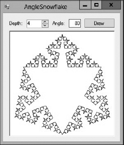
Figure 9-16: Giving the Koch snowflake's generator 80-degree turns creates a spiky result.
- *Write a program that draws Hilbert curves. (For a hint about how to set dx, see Appendix B.)
- Write pseudocode for the algorithms that draw the Sierpi
 ski curve pieces down, left, and up.
 - *Write a program that draws Sierpiski curves. (For a hint about how to set dx, see Appendix B.)
- Write low-level pseudocode to draw the Sierpiski gasket.
- Write low-level pseudocode to draw the Sierpiski carpet.
- Write a program that solves the eight queens problem.
- One improvement you can make to the eight queens problem is to keep track of how many queens can attack a particular position on the board. Then, when you are considering adding a queen to the board, you can ignore any positions where this value isn't 0. Modify the program you wrote for Exercise 12 to use this improvement. How does this improve the number of times the program positions a queen and the total run time?
- To make another improvement to the eight queens problem, notice that every row on the chessboard must hold a single queen. Modify the program you wrote for Exercise 13 so that each call to the EightQueens method searches only the next row for the new queen's position. How does this improve the number of times the program positions a queen, as well as the total run time?
- Write a program that uses only backtracking to solve the knight's tour problem while allowing the user to specify the board's width and height. What is the size of the smallest square board for which a knight's tour is possible?
- Use your favorite programming language to write a program that solves the knight's tour problem by using Warnsdorff's heuristic.
- How are a selection without duplicates and a permutation without duplicates related?
- Write a program that implements the SelectKofNwithDuplicates and SelectKofNwithoutDuplicates algorithms.
- Write a program that implements the PermuteKofNwithDuplicates and PermuteKofNwithoutDuplicates algorithms.
- Write a program that implements the nonrecursive Factorial algorithm.
- Write a program that implements the recursive Fibonacci algorithm with saved values.
- Write a program that implements the non-recursive Fibonacci algorithm.
- The nonrecursive Fibonacci algorithm calculates Fibonacci numbers up to the one it needs and then looks up the value it needs in the array of calculated values. In fact, the algorithm doesn't really need the array. Instead, it can calculate the smaller Fibonacci values whenever they are needed. This takes a little longer but avoids the need for a globally available array. Write a program that implements a nonrecursive Fibonacci algorithm that uses this approach.
- Write a program that implements the nonrecursive Hilbert curve algorithm.