APPENDIX B

Solutions to Exercises

Chapter 1: Algorithm Basics

1. The outer loop still executes O(N) times in the new version of the algorithm. When the outer loop's counter is i, the inner loop executes O(N − i) times. If you add up the number of times the inner loop executes, the result is N + (N − 1) + (N − 2) + ... + 1 = N × (N − 1) / 2 = (N² − N) / 2. This is still O(N²), although the performance in practice will probably be faster than the original version.
2. See Table B-1. The value Infinity means that the program can execute the algorithm for any practical problem size. The example program Ch01Ex02, which is available for download on the book's website, generates these values.

   Table B-1: Maximum Problem Sizes That Run in Various Times

   

3. The question is, “For what N is 1,500 × N > 30 × N²?” Solving for N gives 50 < N, so the first algorithm is slower if N > 50. You would use the first algorithm if N ≤ 50 and the second if N > 50.
4. The question is, “For what N is N³ / 75 − N² / 4 + N + 10 > N / 2 + 8?” You can solve this in any way you like, including algebra or using Newton's method (see Chapter 2). The two positive solutions to this equation are N < 4.92 and N > 15.77. That means you should use the first algorithm if 5 ≥ N ≥ 15. The Ch01Ex04 example program, which is available for download on the book's website, graphs the two equations and uses Newton's method to find their points of intersection.
5. Given N letters, you have N choices for the first letter. After you have picked the first letter, you have N − 1 choices for the second letter, giving you N × (N − 1) total choices. That counts each pair twice (AB and BA), so the total number of unordered pairs is N (N − 1) / 2. In Big O notation that is O(N²).
6. If a cube has side length N, each side has an area of N² units. A cube has six sides, so the total surface area of all sides is 6 × N². If the algorithm generates one value for each square unit, its run time is O(N²).

   Less rigorously, you could have intuitively realized that the cube's surface area depends on N². Therefore, you could conclude that the run time is O(N²) without doing the full calculation.

7. If a cube has side length N, each of its edges has length N. The cube has 12 edges, so the total edge length is 12 × N. However, each of the unit cubes in the corners is part of three edges, so they are counted three times in the 12 × N total. The cube has eight corners, so to make the count correct, you subtract 2 × 8 from 12 × N so that each corner cube is counted only once. The true number of cubes is 12 × N − 16, so the algorithm's run time is O(N).

   Less rigorously, you could have intuitively realized that the total length of the cube's edges depends on N. Therefore, you might conclude that the run time is O(N) without doing the full calculation.

8. Table B-2 shows the number of cubes for several values of N.

   Table B-2: Cubes for Different Values of N

   N	CUBES
   1	1
   2	4
   3	10
   4	20
   5	35
   6	56
   7	84
   8	120

   From the way the shapes grow in length, width, and height in Figure 1-5, you can probably guess that the number of cubes involves N³ in some manner. If you assume the number of cubes is A × N³ + B × N² + C × N + D for some constants A, B, C, and D, you can plug in the values from Table B-2 and solve for A, B, C, and D. If you do that, you'll find that the number of cubes is (N³ + 3 × N² + 2 × N) ÷ 6, so the run time is O(N³).

   Less rigorously, you could have intuitively realized that the total volume of the shapes depends on N³. Therefore, you might conclude that the run time was O(N³) without doing the full calculation.

9. Can you have an algorithm without a data structure? Yes. An algorithm is just a series of instructions, so it doesn't necessarily need a data structure. For example, many of the numeric algorithms described in Chapter 2 do not use data structures.

   Can you have a data structure without an algorithm? Not really. You need some sort of algorithm to build the data structure, and you need another algorithm to use it to produce some kind of result. There isn't much point to a data structure that you won't use to produce a result.

10. The first algorithm simply paints the boards from one end to the other. It paints N boards and therefore has a run time of O(N).

    The second algorithm divides the boards in a recursive way, but eventually it paints all N boards. Dividing the boards recursively requires O(log N) steps. Painting the boards requires O(N) steps. The total number of steps is N + log N, so the run time is O(N), just like the first algorithm.

    The algorithms have the same run time, but the second takes slightly longer in practice if not in Big O notation. It is also more complicated and confusing, so the first algorithm is better.

11. Figure B-1 shows the Fibonacci function graphed with the other runtime functions. If you look closely at the figure, you can tell that Fibonacci(x) ÷ 10 curves up more steeply than x² ÷ 5 and slightly less steeply than 2^× ÷ 10. The shape of its curve is very similar to the shape of 2^× ÷ 10, so you might guess (correctly) that it is an exponential function.

Figure B-1: The Fibonacci function increases more quickly than x² but less quickly than 2^×.

It turns out that you can calculate the Fibonacci numbers directly using the following formula:

Fibonacci (n) =

where:

So the Fibonacci function is exponential in φ. The value φ ≈ 1.618, so the function doesn't grow as quickly as 2^N, but it is still exponential and does grow faster than polynomial functions.

Chapter 2: Numerical Algorithms

1. Simply map 1, 2, and 3 to heads and 4, 5, and 6 to tails.
2. In this case, the probability of getting heads followed by heads is 3 ÷ 4 × 3 ÷ 4 = 9 ÷ 16. The probability of getting tails followed by tails is 1 ÷ 4 × 1 ÷ 4 = 1 ÷ 16. Because these are independent outcomes, you can add their probabilities. So there is a 9 ÷ 16 + 1 ÷ 16 = 10 ÷ 16 = 0.625, or 62.5%, probability that you'll need to try again.
3. If the coin is fair, the probability that you'll get heads followed by heads is 1 ÷ 2 × 1 ÷ 2 = 1 ÷ 4. Similarly, the probability that you'll get tails followed by tails is 1 ÷ 2 × 1 ÷ 2 = 1 ÷ 4. Because these are independent outcomes, you can add their probabilities. So there is a 1 ÷ 4 + 1 ÷ 4 = 1 ÷ 2, or 50%, probability that you'll need to try again.
4. You can use a method similar to the one that uses a biased coin to produce fair coin flips:

   Roll the biased die 6 times. If the rolls include all 6 possible values, return the first one. Otherwise, repeat.

   Depending on how biased the die is, it could take many trials to roll all six values. For example, if the die is fair (the best case), the probability of rolling all six values is 6! ÷ 6⁶ = 720 ÷ 46,656 ≈ 0.015, so there's only about a 1.5% chance that six rolls will give six different values. For another example, if the die rolls a 1 half of the time and each of the other five values one-tenth of the time, the probability of getting all six values in six rolls is 0.5 × 0.1⁵ × 6! = 0.0036, or 0.36%. So you may be rolling the die for a long time.

5. You can use the same algorithm to randomize an array, but you can stop after positioning the first M items:

   String: PickM(String: array[], Integer: M) Integer: max_i = <Upper bound of array> For i = 0 To M − 1 // Pick the item for position i in the array. Integer: j = <pseudo-random number between i and max_i inclusive> <Swap the values of array[i] and array[j]> Next i <Return array[0] through array[M − 1]> End PickM

   This algorithm runs in O(M) time. Because M ≤ N, O(M) ≤ O(N). In practice, M is often much less than N, so this algorithm may be much faster than randomizing the entire array.

   To give away five books, you would pick five names to go in the array's first five positions and then stop. This would take only five steps, so it would be very quick. It doesn't matter how many names are in the array, as long as there are at least five.

6. Simply make an array holding all 52 cards, randomize it, and then deal the cards as you normally would—one to each player in turn until everyone has five.

   It doesn't matter whether you deal one card to each player in turn or deal five cards all at once to each player. As long as the deck is randomized, each player will get five randomly selected cards.

7. Figure B-2 shows the program written in C#, which is available for download on the book's website. The numbers for each value are the actual percentage of rolls that gave the value, the expected percentage for the value, and the percentage difference.

   

   Figure B-2: Relatively small numbers of trials sometimes result in significant differences between observed and expected frequencies of rolls.

   The actual results don't consistently match the expected results until the number of trials is quite large. The program often produces more than 5% error for some values until about 10,000 or more trials are run.

8. If A₁ < B₁, A₁ Mod B₁ = A₁, so A₂ = B₁ and B₂ = A₁ Mod B₁ = A₁. In other words, during the first trip through the While loop, the values of A and B switch. After that the algorithm proceeds normally.
9. LCD(A, B) = A × B / GCD(A, B). Suppose g = GCD(A, B), so A = g × m and B = g × n for some integers m and n. Then A × B ÷ GCD(A, B) = g × m × g × n ÷ g = g × m × n. The values m and n have no common factors, so this is the LCM.
10. The following pseudocode shows the algorithm used by the FastExponentiation example program that's available for download on the book's website. (The bold lines of code are used for the solution to Exercise 11.)

    // Perform the exponentiation. Integer: Exponentiate(Integer: value, Integer: exponent) // Make lists of powers and the value to that power. List Of Integer: powers List Of Integer: value_to_powers // Start with the power 1 and value^1. Integer: last_power = 1 Integer: last_value = value powers.Add(last_power) value_to_powers.Add(last_value) // Calculate other powers until we get to one bigger than exponent. While (last_power < exponent) last_power = last_power * 2 last_value = last_value * last_value powers.Add(last_power) value_to_powers.Add(last_value) End While // Combine values to make the required power. Integer: result = 1 // Get the index of the largest power that is smaller than exponent. For power_index = powers.Count - 1 To 0 Step −1 // See if this power fits within exponent. If (powers[power_index] <= exponent) // It fits. Use this power. exponent = exponent - powers[power_index] result = result * value_to_powers[power_index] End If Next power_index // Return the result. Return result End Exponentiate

11. You would need to modify the bold lines in the preceding code. If the modulus is m, you would change this line:

    last_value = last_value * last_value

    to this:

    last_value = (last_value * last_value) Modulus m

    You would also change this line:

    result = result * value_to_powers[power_index]

    to this:

    result = (result * value_to_powers[power_index]) Modulus m

    The ExponentiateMod example program that's available for download on the book's website demonstrates this algorithm.

12. Figure B-3 shows the GcdTimes example program that is available for download on the book's website. The gray lines show the graph of number of steps versus values. The dark curve near the top shows the logarithm of the values. It's hard to tell from the graph if the number of steps really follows the logarithm, but it clearly grows very slowly.

    

    Figure B-3: The GcdTimes example program graphs number of GCD steps versus number size.

13. You already know that next_prime × 2 has been crossed out, because it is a multiple of 2. If next_prime > 3, you know that next_prime × 3 has also been crossed out, because 3 has already been considered. In fact, for every prime p where p < next_prime, the prime p has already been considered, so next_prime × p has already been crossed out. The first prime that is not less than next_prime is next_prime, so the first multiple of next_prime that has not yet been considered is next_prime × next_prime. That means you can change the loop to the following:

    // "Cross out" multiples of this prime. For i = next_prime * next_prime To max_number Step next_prime Then is_composite[i] = true Next i

14. The following pseudocode shows an algorithm to display Carmichael numbers and their prime factors:

    // Generate Carmichael numbers. GenerateCarmichaelNumbers(Integer: max_number) Boolean: is_composite[] <Make is_composite a sieve of Eratosthenes for numbers 2 through max_number> // Check for Carmichael numbers. For i = 2 To max_number // Only check nonprimes. If (is_composite[i]) Then // See if i is a Carmichael number. If (IsCarmichael(i)) Then <Output i and its prime factors> End If End If Next i End GenerateCarmichaelNumbers // Return true if the number is a Carmichael number. Boolean: IsCarmichael(Integer: number) // Check all possible witnesses. For i = 1 to number - 1 // Only check numbers with GCD(number, 1) = 1. If (GCD(number, i) == 1) Then <Use fast exponentiation to calculate i ^ (number-1) mod number> Integer: result = Exponentiate(i, number - 1, number) // If we found a Fermat witness, // this is not a Carmichael number. If (result != 1) Then Return false End If Next i // They're all a bunch of liars! // This is a Carmichael number. Return true End IsCarmichael

    You can download the CarmichaelNumbers example program from the book's website to see a C# implementation of this algorithm.

15. Suppose you use the value of the function at the rectangle's midpoint for the rectangle's height. Then, if the function is increasing, the left part of the rectangle is too short, and the right part is too tall, so the error in the two pieces tends to cancel out, at least to some extent. Similarly, if the function is decreasing, the left part of the rectangle is too short, and the right part is too tall, so again they partially cancel each other out. This reduces the total error considerably without increasing the number of rectangles.

    This method won't help (and may even hurt) if the curve has a local minimum or maximum near the middle of a rectangle. In those cases the errors on the left and right sides of the curve will add up and give a larger total error.

    Figure B-4 shows the MidpointRectangleRule example program, which is available for download on the book's website, demonstrating this technique. If you compare the result to the one shown in Figure 2-2, you'll see that using the midpoint reduced the total error from about −6.5% to 0.2%, roughly 1/30th of the error, without changing the number of rectangles.

    

    Figure B-4: The MidpointRectangleRule example program reduces error by using each rectangle's midpoint to calculate its height.

16. Yes. This would be similar to a version of the AdaptiveGridIntegration program that would use pseudorandom points instead of a grid. If done properly, it would be more effective than a normal Monte Carlo integration, because it would pick more points in areas of interest and fewer in large areas that are either all in or all out of the shape.
17. The following pseudocode shows a high-level algorithm for performing Monte Carlo integration in three dimensions:

    Float: EstimateVolume(Boolean: PointIsInShape(,,), Integer: num_trials, Float: xmin, Float: xmax, Float: ymin, Float: ymax, Float: zmin, Float: zmax) Integer: num_hits = 0 For i = 1 To num_trials Float: x = <pseudorandom number between xmin and xmax> Float: y = <pseudorandom number between ymin and ymax> Float: z = <pseudorandom number between zmin and zmax> If (PointIsInShape(x, y, z)) Then num_hits = num_hits + 1 Next i Float: total_volume = (xmax − xmin) * (ymax − ymin) * (zmax − zmin) Float: hit_fraction = num_hits / num_trials * Return total_volume * hit_fraction End EstimateVolume

18. To find the points of intersection between the functions y = f(x) and y = g(x), you can use Newton's method to find the roots of the equation y = f(x) − g(x). Those roots are the X values where f(x) and g(x) intersect.

Chapter 3: Linked Lists

1. Assuming that the program has a pointer bottom that points to the last item in a linked list, the following pseudocode shows how you could add an item to the end of the list:

   Cell: AddAtEnd(Cell: bottom, Cell: new_cell) bottom.Next = new_cell new_cell.Next = null // Return the new bottom cell. Return new_cell End AddAtEnd

   This algorithm returns the new bottom cell, so the calling code can update the variable that points to the list's last cell. Alternatively, you could pass the bottom pointer into the algorithm by reference so that the algorithm can update it.

   Using a bottom pointer doesn't change the algorithms for adding an item at the beginning of the list or for finding an item.

   Removing an item is the same as before unless that item is at the end of the list, in which case you also need to update the bottom pointer. Because you identify the item to be removed with a pointer to the item before it, this is a simple change. The following code shows the modified algorithm for removing the last item in the list:

   Cell: DeleteAfter(Cell: after_me, Cell: bottom) // If the cell being removed is the last one, update bottom. If (after_me.Next.Next == null) Then bottom = after_me // Remove the target cell. after_me.Next = after_me.Next.Next // Return a pointer to the last cell. Return bottom End DeleteAfter

2. The following pseudocode shows an algorithm for finding the largest cell in a singly linked list with cells containing integers:

   Cell: FindLargestCell(Cell: top) // If the list is empty, return null. If (top.Next == null) Return null // Move to the first cell that holds data. top = top.Next // Save this cell and its value. Cell: best_cell = top Integer: best_value = best_cell.Value // Move to the next cell. top = top.Next // Check the other cells. While (top != null) // See if this cell's value is bigger. If (top.Value > best_value) Then best_cell = top best_value = top.Value End If // Move to the next cell. top = top.Next End While Return best_cell End FindLargestCell

3. The following pseudocode shows an algorithm to add an item at the top of a doubly linked list:

   AddAtBeginning(Cell: top, Cell: new_cell) // Update the Next links. new_cell.Next = top.Next top.Next = new_cell // Update the Prev links. new_cell.Next.Prev = new_cell new_cell.Prev = top End AddAtBeginning

4. The following pseudocode shows an algorithm to add an item at the bottom of a doubly linked list:

   AddAtEnd(Cell: bottom, Cell: new_cell) // Update the Prev links. new_cell.Prev = bottom.Prev bottom.Prev = new_cell // Update the Next links. new_cell.Prev.Next = new_cell new_cell.Next = bottom End AddAtEnd

5. The InsertCell algorithm takes as a parameter the cell after which the new cell should be inserted. All the AddAtBeginning and AddAtEnd algorithms need to do is pass InsertCell the appropriate cell to insert after. The following code shows the new algorithms:

   AddAtBeginning(Cell: top, Cell: new_cell) // Insert after the top sentinel. InsertCell(top, new_cell) End AddAtBeginning AddAtEnd(Cell: bottom, Cell: new_cell) // Insert after the cell before the bottom sentinel. InsertCell(bottom.Prev, new_cell) End AddAtEnd

6. The following pseudocode shows an algorithm that deletes a specified cell from a doubly linked list:

   DeleteCell(Cell: target_cell) // Update the next cell's Prev link. target_cell.Next.Prev = target_cell.Prev // Update the previous cell's Next link. target_cell.Prev.Next = target_cell.Next End DeleteCell

   Figure B-5 shows the process graphically.

   

   Figure B-5: To delete a cell from a doubly linked list, change the next and previous cells' links to “go around” the target cell.

7. If the name you're looking for comes nearer the end of the alphabet than the beginning, such as a name that starts with N or later, you could search the list backwards, starting at the bottom sentinel. This would not change the O(N) run time, but it might cut the search time roughly in half in practice if the names are reasonably evenly distributed.
8. The following pseudocode shows an algorithm for inserting a cell in a sorted doubly linked list:

   // Insert a cell in a sorted doubly linked list. InsertCell(Cell: top, Cell: new_cell) // Find the cell before where the new cell belongs. While (top.Next.Value < new_cell.Value) top = top.Next End While // Update Next links. new_cell.Next = top.Next top.Next = new_cell // Update Prev links. new_cell.Next.Prev = new_cell new_cell.Prev = top End InsertCell

   This algorithm is similar to the one used for a singly linked list except for the two lines that update the Prev links.

9. The following pseudocode determines whether a linked list is sorted:

   Boolean: IsSorted(Cell: sentinel) // If the list has 0 or 1 items, it's sorted. If (sentinel.Next == null) Then Return true If (sentinel.Next.Next == null) Then Return true // Compare the other items. sentinel = sentinel.Next; While (sentinel.Next != null) // Compare this item with the next one. If (sentinel.Value > sentinel.Next.Value) Then Return false // Move to the next item. sentinel = sentinel.Next End While // If we get here, the list is sorted. Return true End IsSorted

10. Insertionsort takes the first item from the input list and then finds the place in the growing sorted list where that item belongs. Depending on its value, sometimes the item will belong near the beginning of the list, and sometimes it will belong near the end. The algorithm won't always need to search the whole list, unless the new item is larger than all the items already on the sorted list.

    In contrast, when selectionsort searches the unsorted input list to find the largest item, it must search the whole list. Unlike insertionsort, it can never stop the search early.

11. The PlanetList example program, which is available for download on the book's website, shows one solution.
12. The BreakLoopTortoiseAndHare example program, which is available for download on the book's website, shows a C# solution.

Chapter 4: Arrays

1. The following algorithm calculates an array's sample variance:

   Double: FindSampleVariance(Integer: array[]) // Find the average. Integer: total = 0 For i = 0 To array.Length - 1 total = total + array[i] Next i Double: average = total / array.Length // Find the sample variance. Double: sum_of_squares = 0 For i = 0 To array.Length − 1 sum_of_squares = sum_of_squares + (array[i] − average) * (array[i] − average) Next i Return sum_of_squares / array.Length End FindSampleVariance

2. The following algorithm uses the preceding algorithm to calculate sample standard deviation:

   Integer: FindSampleStandardDeviation(Integer: array[]) // Find the sample variance. Double: variance = FindSampleVariance(array) // Return the standard deviation. Return Sqrt(variance) End FindSampleStandardDeviation

3. Because the array is sorted, the median is the item in the middle of the array. You have two issues to think about. First, you need to handle arrays with even and odd lengths differently. Second, you need to be careful calculating the index of the middle item, keeping in mind that indexing starts at 0.

   Double: FindMedian(Integer: array[]) If (array.Length Mod 2 == 0) Then // The array has even length. // Return the average of the two middle items. Integer: middle = array.Length / 2 Return (array[middle − 1] + array[middle]) / 2 Else // The array has odd length. // Return the middle item. Integer: middle = (array.Length − 1)/ 2 Return array[middle] End If End FindMedian

4. The following pseudocode removes an item from a linear array:

   RemoveItem(Integer: array[], Integer: index) // Slide items left 1 position to fill in where the item is. For i = index + 1 To array.Length − 1 Array[i − 1] = Array[i] Next i // Resize to remove the final unused entry. <Resize the array to delete 1 item from the end> End RemoveItem

5. All you really need to change in the original triangular array class is the method that uses row and column to calculate the index in the one-dimensional storage array. The following pseudocode shows the original method:

   Integer: FindIndex(Integer: r, Integer: c) Return ((r − 1) * (r − 1) + (r − 1)) / 2 + c End FindIndex

   The following pseudocode shows the new version with row and column switched:

   Integer: FindIndex(Integer: r, Integer: c) Return ((c − 1) * (c − 1) + (c − 1)) / 2 + r End FindIndex

6. The relationship between row and column for nonblank entries in an N×N array is row + column < N. You could rework the equation for mapping row and column to an index in the one-dimensional storage array, but it's easier to map the row and column to a new row and column that fit the original lower-left triangular arrangement. You can do this by replacing r with N − 1 − r, as shown in the following pseudocode:

   Integer: FindIndex(Integer: r, Integer: c) r = N − 1 − r Return ((r − 1) * (r − 1) + (r − 1)) / 2 + c End FindIndex

   This change essentially flips the array upside-down so that small row numbers are mapped to the bottom of the array and large row numbers are mapped to the top of the array. For example, suppose N = 5. Then the entry [0, 4] is in the upper-right corner of the array. That position is not allowed in the normal lower-left triangular array, so the row is changed to N − 1 − 0 = 4. The position [4, 4] is in the lower right corner, which is in the normal array.

7. The following pseudocode fills the array with the values ll_value and ur_value. You can set these to 1 and 0 to get the desired result.

   FillArrayLLtoUR(Integer: values[,], Integer: ll_value, Integer: ur_value) For row = 0 To <Upper bound for dimension 1> For col = 0 To <Upper bound for dimension 2> If (row >= col) Then values[row, col] = ur_value Else values[row, col] = ll_value End If Next col Next row End FillArrayLLtoUR

8. The following pseudocode fills the array with the values ul_value and lr_value. You can set these to 1 and 0 to get the desired result.

   FillArrayULtoLR(Integer: values[,], Integer: ul_value, Integer: lr_value) Integer: max_col = <Upper bound for dimension 2> For row = 0 To <Upper_bound for dimension 1> For col = 0 To max_col If (row > max_col − col) Then values[row, col] = ul_value Else values[row, col] = lr_value End If Next col Next row End FillArrayULtoLR

9. One approach is to set the value for each entry in the array to the minimum of its row, column, and distance to the right and lower edges of the array, as shown in the following pseudocode:

   FillArrayWithDistances(Integer: values[,]) Integer: max_row = values.GetUpperBound(0) Integer: max_col = values.GetUpperBound(1) For row = 0 To max_row For col = 0 To max_col values[row, col] = Minimum(row, col, max_row − row, max_col − col) Next col Next row End FillArrayWithDistances

10. The key is the mapping between [row, column, height] and indices in the storage array. To do that, the program needs to know how many cells are in a full tetrahedral group of cells and how many cells are in a full triangular group of cells. Chapter 4 explains that the number of cells in a full triangular arrangement is (N² + N) ÷ 2, so the following pseudocode can calculate that value:

    Integer: NumCellsForTriangleRows(Integer: rows) Return (rows * rows + rows) / 2 End NumCellsForTriangleRows

    The number of cells in a full tetrahedral arrangement is harder to calculate. If you make some drawings and count the cells, you can follow the approach used in the chapter. (See Table 4-1 and the nearby paragraphs.) If you assume the number of cells in the tetrahedral arrangement involves the number of rows cubed, you will find that the exact number is (N³ + 3 × N² + 2 × N) / 6. The following pseudocode uses that formula:

    Integer: NumCellsForTetrahedralRows(Integer: rows) Return (rows * rows * rows + 3 * rows * rows + 2 * rows) / 6 End NumCellsForTetrahedralRows

    With these two methods, you can write a method to map [row, column, height] to an index in the storage array:

    Integer: RowColumnHeightToIndex(Integer: row, Integer: col, Integer: hgt) Return NumCellsForTetrahedralRows(row) + NumCellsForTriangleRows(col) + hgt; End RowColumnHeightToIndex

    This code returns the number of entries before this one in the array. It calculates that number by adding the entries due to complete tetrahedral groups before this item, plus the number of entries due to complete triangular groups before this item, plus the number of individual entries that come before this one in its triangular group of cells.

11. The sparse array already doesn't use space to hold missing entries, so this isn't as matter of rearranging the data structure to save space. All you really need to do is check that row ≥ column when you access an entry.
12. You can add two triangular arrays by simply adding corresponding items. The only trick here is that you only need to consider entries where row ≥ column. The following pseudocode does this:

    AddTriangularArrays(Integer: array1[,], Integer: array2[,], Integer: result[,]) For row = 0 To <Upper bound for dimension 1> For col = 0 To row Result[row, col] = array1[row, col] + array2[row, col] Next col Next row End AddTriangularArrays

13. The following code for multiplying two matrices was shown in the chapter's text:

    MultiplyArrays(Integer: array1[], Integer: array2[], Integer: result[]) For i = 0 To <Upper bound for dimension 1> For j = 0 To <Upper bound for dimension 2> // Calculate the [i, j] result. result[i, j] = 0 For k = 0 To <Upper bound for dimension 2> result[i, j] = result[i, j] + array1[i, k] * array2[k, j] Next k Next j Next i End MultiplyArrays

    Now consider the inner For k loop. If i < k, array1[i, k] is 0. Similarly, if k < j, array2[k, j] is 0. If either of those two values is 0, their product is 0.

    The following code shows how you can modify the inner assignment statement so that it changes an entry's value only if it is multiplying entries that are present in both arrays:

    If (i >= k) And (k >= j) Then result[i, j] = result[i, j] + array1[i, k] * array2[k, j] End If

    You can make this a bit simpler if you think about the values of k that access entries that exist in both arrays. Those values exist if k <= i and k >= j. You can use those bounds for k in its For loop, as shown in the following pseudocode:

    For k = j To i total += this[i, k] * other[k, j]; Next k

14. The following code shows a CopyEntries method that copies the items in the ArrayEntry linked list starting at from_entry to the end of the list that currently ends at to_entry:

    // Copy the entries starting at from_entry into // the destination entry list after to_entry. CopyEntries(ArrayEntry: from_entry, ArrayEntry: to_entry) While (from_entry != null) to_entry.NextEntry = new ArrayEntry to_entry = to_entry.NextEntry to_entry.ColumnNumber = from_entry.ColumnNumber to_entry.Value = from_entry.Value to_entry.NextEntry = null // Move to the next entry. from_entry = from_entry.NextEntry End While End CopyEntries

    As long as the “from” list isn't empty, this adds a new ArrayEntry object to the “to” list.

    The following AddEntries method copies entries from the two lists from_entry1 and from_entry2 into the result list to_entry:

    // Add the entries in the two lists from_entry1 and from_entry2 // and save the sums in the destination entry list after to_entry. AddEntries(ArrayEntry: from_entry1, ArrayEntry: from_entry2, ArrayEntry: to_entry) // Repeat as long as either from list has items. While (from_entry1 != null) And (from_entry2 != null) // Make the new result entry. to_entry.NextEntry = new ArrayEntry to_entry = to_entry.NextEntry to_entry.NextEntry = null // See which column number is smaller. If (from_entry1.ColumnNumber < from_entry2.ColumnNumber) Then // Copy the from_entry1 entry. to_entry.ColumnNumber = from_entry1.ColumnNumber to_entry.Value = from_entry1.Value from_entry1 = from_entry1.NextEntry Else If (from_entry2.ColumnNumber < from_entry1.ColumnNumber) Then // Copy the from_entry2 entry. to_entry.ColumnNumber = from_entry2.ColumnNumber to_entry.Value = from_entry2.Value from_entry2 = from_entry2.NextEntry Else // The column numbers are the same. Add both entries. to_entry.ColumnNumber = from_entry1.ColumnNumber to_entry.Value = from_entry1.Value + from_entry2.Value from_entry1 = from_entry1.NextEntry from_entry2 = from_entry2.NextEntry End If End While // Add the rest of the entries from the list that is not empty. if (from_entry1 != null) CopyEntries(from_entry1, to_entry) if (from_entry2 != null) CopyEntries(from_entry2, to_entry) End AddEntries

    This code loops through both “from” lists, adding the next entry from each list that has the smaller column number. If the current entries in each list have the same column number, the code creates a new entry and adds the values of the “from” lists.

    The following code shows how the Add method uses CopyEntries and AddEntries to add two matrices:

    // Add two SparseArrays representing matrices. SparseArray: Add(SparseArray: array1, SparseArray: array2) SparseArray: result = new SparseArray // Variables to move through all the arrays. ArrayRow: array1_row = array1.TopSentinel.NextRow ArrayRow: array2_row = array2.TopSentinel.NextRow ArrayRow: result_row = result.TopSentinel While (array1_row != null) And (array2_row != null) // Make a new result row. result_row.NextRow = new ArrayRow result_row = result_row.NextRow result_row.RowSentinel = new ArrayEntry result_row.NextRow = null // See which input row has the smaller row number. If (array1_row.RowNumber < array2_row.RowNumber) Then // array1_row comes first. Copy its values into result. result_row.RowNumber = array1_row.RowNumber CopyEntries(array1_row.RowSentinel.NextEntry, result_row.RowSentinel) array1_row = array1_row.NextRow Else If (array2_row.RowNumber < array1_row.RowNumber) Then // array2_row comes first. Copy its values into result. result_row.RowNumber = array2_row.RowNumber CopyEntries(array2_row.RowSentinel.NextEntry, result_row.RowSentinel) array2_row = array2_row.NextRow Else // The row numbers are the same. Add their values. result_row.RowNumber = array1_row.RowNumber AddEntries( array1_row.RowSentinel.NextEntry, array2_row.RowSentinel.NextEntry, result_row.RowSentinel) array1_row = array1_row.NextRow array2_row = array2_row.NextRow End If End While // Add any remaining rows. If (array1_row != null) Then // Make a new result row. result_row.NextRow = new ArrayRow result_row = result_row.NextRow result_row.RowNumber = array1_row.RowNumber result_row.RowSentinel = new ArrayEntry result_row.NextRow = null CopyEntries(array1_row.RowSentinel.NextEntry, result_row.RowSentinel) End If If (array2_row != null) Then // Make a new result row. result_row.NextRow = new ArrayRow result_row = result_row.NextRow result_row.RowNumber = array2_row.RowNumber result_row.RowSentinel = new ArrayEntry result_row.NextRow = null CopyEntries(array2_row.RowSentinel.NextEntry, result_row.RowSentinel) End If return result End Add

    The method loops through the two “from” arrays. If one list's current row has a lower row number than the other, the method uses CopyEntries to copy that row's entries into the “to” list.

    If the lists' current rows have the same row number, the method uses AddEntries to combine the rows in the output array.

    After one of the “from” lists is empty, the method uses CopyEntries to copy the remaining items in the other “from” list into the output list.

15. To multiply two matrices, you need to multiply the rows of the first with the columns of the second. To do that efficiently, you need to be able to iterate over the entries in the second array's columns. The sparse arrays described in the text let you iterate over the entries in their rows but not the entries in the columns.

    You can make it easier to iterate over the entries in a column by using a linked list of columns, each holding a linked list of entries, just as the text describes using linked lists of rows.

    Instead of building a whole new class, however, you can reuse the existing SparseArray class. If you reverse the roles of the rows and columns, you get an equivalent array that lets you traverse the fields in a column. Of course, the class will treat the rows as columns and vice versa, so this can be confusing.

    The following pseudocode shows a high-level algorithm for multiplying two sparse matrices:

    Multiply(SparseArray: array1, SparseArray: array2, SparseArray: result) // Make a column-major version of array2. SparseArray: new_array2 For Each entry [i, j] in array2 new_array2[j, i] = array2[i, j] Next [i, j] // Multiply. For Each row number r in array1 For Each "row" number c in array2 // These are really columns. Integer: total = 0 For Each <k that appears in both array1's row and array2's column> total = total + <The row's k value> * <the column's k value> Next k result[r, c] = total Next c Next r End Multiply

Chapter 5: Stacks and Queues

1. When one of the stacks is full, NextIndex1 > NextIndex2. At that point both stacks are full, NextIndex1 is the index of the top item in the second stack, and NextIndex2 is the index of the top item in the first stack.
2. Simply push each of the items from the original stack onto a new one. The following pseudocode shows this algorithm:

   Stack: ReverseStack(Stack: values) Stack: new_stack While (<values is not empty>) new_stack.Push(values.Pop()) End While Return new_stack End ReverseStack

3. The StackInsertionsort example program, which is available for download on the book's website, demonstrates insertionsort with stacks.
4. The algorithm doesn't really need to move all the unsorted items back onto the original stack, because all it will do with those items is take the next one to insert in sorted position. Instead, the algorithm could just move the sorted items back onto the original stack and then use the next unsorted item as the next item to position. This would save some time, but the run time would still be O(N²).
5. The fact that the stack insertionsort algorithm works means that you can sort train cars with only one holding track plus the output track. You can use the holding track as the second stack, and you can use the output track to store the car you are currently sorting (or vice versa). This would require more steps than you would need if you have more than one holding track, however. Because moving train cars is a lot slower than moving items between stacks on a computer, it would be better to use more holding tracks if possible.
6. The StackSelectionsort example program, which is available for download on the book's website, demonstrates selectionsort with stacks.
7. You can use the selectionsort algorithm to sort train cars with some small modifications. The version described in Chapter 5 keeps track of the largest item in a separate variable. When sorting train cars, you can't set aside a car to hold in a variable. Instead, you can move cars to the holding track and store the car with the largest number on the output track. When you find a car with a larger number, you can move the car from the output track back to the holding track and then move the new car to the output track.

   Of course, with real trains, you don't need to look only at the top car in a stack. Instead, you can look at the unsorted cars and figure out which has the largest number before you start moving any cars. Then you can simply move the cars to the holding track, except for the selected car, which you can move to the output track. That will remove any need to put incorrect cars on the output track and reduce time-consuming shuffling.

8. The InsertionsortPriorityQueue example program, which is available for download on the book's website, uses a linked list to implement a priority queue.
9. The LinkedListDeque example program, which is available for download on the book's website, uses a doubly linked list to implement a deque.
10. The MultiHeadedQueue example program, which is available for download on the book's website, demonstrates a multiheaded queue.

    The average wait time is very sensitive to the number of tellers. If you have even one fewer than the optimum number of tellers, the number of customers in the queue quickly grows long, and the average wait time soars. Adding a single teller can make the queue practically disappear and reduce average wait time to only a few seconds. (Some retailers have learned this lesson. Whenever more than a couple of customers are waiting, pull employees from other jobs to open a new register and quickly clear the queue.)

11. The QueueInsertionsort example program does this.
12. The QueueSelectionsort example program does this.

Chapter 6: Sorting

For performance reasons, all of the sorting example programs display at most 1,000 of the items they are sorting. If the program generates more than 1,000 items, all of the items are processed but only the first 1,000 are displayed in the output list.

1. Example program Insertionsort implements the insertionsort algorithm.
2. When the algorithm starts with index 0, it moves the 0th item to position 0, so it doesn't change anything. Making the algorithm's For loop start at 1 instead of 0 essentially makes it treat the first item as already in sorted position. That makes sense, because a group of one item is already sorted.

   Starting the loop at 1 doesn't change the algorithm's run time.

3. Example program Selectionsort implements the selectionsort algorithm.
4. The algorithm's outer For loop could stop before the last item in the array, because the final trip through the loop positions the item at position N − 1 at index N − 1, so it isn't moved anyway. The following pseudocode shows the new For statement:

   For i = 0 To <length of values> − 2

   This would not change the algorithm's run time.

5. Example program Bubblesort implements the bubblesort algorithm.
6. Example program ImprovedBubblesort adds those improvements.
7. Example program PriorityQueue uses a heap to implement a priority queue. (This program works directly with the value and priority arrays. For more practice, package the heap code into a class.)
8. Adding an item to and removing an item from a heap containing N items take O(log N) time. See the discussion of the heapsort algorithm's run time for details.
9. Example program Heapsort implements the heapsort algorithm.
10. For a complete tree of degree d, if a node has index p, its children are at d × p + 1, d × p + 2, and d × p + 3. A node at index p has parent index (p − 1)/d.
11. Example program QuicksortStack implements the quicksort algorithm with stacks.
12. Example program QuicksortQueue implements the quicksort algorithm with queues. Stacks and queues provide the same performance as far as the quicksort algorithm is concerned. Any difference would be in how the stacks and queues are implemented.
13. Example program Quicksort implements the quicksort algorithm with in-place partitioning.
14. Instead of dividing the items into two halves at each step, divide them into three groups. The first group contains items strictly less than the dividing item, the middle group contains all repetitions of the dividing item, and the last group contains items greater than the dividing item. Then recursively sort the first and third groups but not the second.
15. Example program Countingsort implements the countingsort algorithm.
16. Allocate a counts array with indices 0 to 10,000. Subtract the smallest item's value (100,000) from each item before you increment its count. Then, when you are writing the counts back into the original array, add 100,000 back in. (Alternatively, you could use an array with nonzero lower bounds, as described in Chapter 4.)
17. In this case bucketsort almost becomes countingsort. Bucketsort would need to sort each bucket, but all the items in a particular bucket would have the same value. As long as the buckets don't hold too many items, that's not a problem, but countingsort still has a small advantage, because it only needs to count the items in each bucket.
18. Example program Bucketsort implements the bucketsort algorithm.
19. The following paragraphs explain which algorithms would work well under the indicated circumstances.
    1. 10 floating-point values—Any of the algorithms except countingsort would work. Insertionsort, selectionsort, and bubblesort would be simplest and would probably provide the best performance.
    2. 1,000 integers—Heapsort, quicksort, and mergesort would work well. Quicksort would be fastest if the values don't contain too many duplicates and are not initially sorted or you use a randomized method for selecting dividing items. Countingsort would work if the range of values is limited.
    3. 1,000 names—Heapsort, quicksort, and mergesort would work well. Quicksort would be fastest if the values don't contain too many duplicates and are not initially sorted or you use a randomized method for selecting dividing items. Countingsort won't work. Making bucketsort work might be difficult. (The trie described in Chapter 10 is similar to a bucketsort, and it would work.)
    4. 100,000 integers with values between 0 and 1,000—Countingsort would work very well. Bucketsort would also work well, but not as well as countingsort. Heapsort, quicksort, and mergesort would work but would be slower.
    5. 100,000 integers with values between 0 and 1 billion—Countingsort would not work very well, because it would need to allocate an array with 1 billion entries to hold value counts. Bucketsort would work well. Heapsort, quicksort, and mergesort would work but would be slower.
    6. 100,000 names—Countingsort doesn't work with strings. Making bucketsort work might be difficult. (Again, the trie described in Chapter 10 would work.) Heapsort, quicksort, and mergesort would work well, with quicksort being the fastest in the expected case.
    7. 1 million floating-point values—Countingsort doesn't work with strings. Bucketsort would work well. Heapsort, quicksort, and mergesort would work but would be much slower.
    8. 1 million names—This is a hard one for the algorithms described in this chapter. Countingsort doesn't work with strings. Making bucketsort work with strings could be hard, but it would work. Heapsort, quicksort, and mergesort would work but would be slow. The trees described in Chapter 10 can also handle this case.
    9. 1 million integers with uniform distribution—Countingsort might work if the range of values is limited. Otherwise, bucketsort would probably be the best choice. Heapsort, quicksort, and mergesort would work but would be slow.
    10. 1 million integers with nonuniform distribution—Countingsort might work if the range of values is limited. Bucketsort might have trouble because the distribution is nonuniform. Heapsort, quicksort, and mergesort would work but would be slow.

Chapter 7: Searching

1. Example program LinearSearch implements the linear search algorithm.
2. Example program RecursiveLinearSearch implements the linear search algorithm recursively. If the array holds N items, this method might require N levels of recursion. Some programming languages may be unable to handle that depth of recursion for large N, so the nonrecursive version probably is safer.
3. Example program LinearLinkedListSearch implements the linear search algorithm for a linked list.
4. Example program BinarySearch implements the binary search algorithm.
5. Example program RecursiveBinarySearch implements the binary search algorithm recursively. This method requires more stack space than the nonrecursive version. That could be a problem if the depth of recursion is great, but that would occur only for extremely large arrays, so it probably isn't an issue in practice. That being the case, the better algorithm is the one you find less confusing. (Personally, I think the nonrecursive version is less confusing.)
6. Example program InterpolationSearch implements the interpolation search algorithm.
7. Example program RecursiveInterpolationSearch implements the interpolation search algorithm recursively. As is the case with binary search, this method requires more stack space than the nonrecursive version. That could be a problem if the depth of recursion is great, but that would occur only for extremely large arrays, so it probably isn't an issue in practice. That being the case, the better algorithm is the one you find less confusing. (Personally, I think the nonrecursive version is less confusing.)
8. The bucketsort algorithm uses a calculation similar to the one used by interpolation search to pick each item's bucket.
9. You could simply move backwards through the array until you find the first item that doesn't match the target. In the worst case, that would take O(N) time. For example, if a program used binary search on an array that contained nothing but copies of the target item, the algorithm would find the target halfway through the array and then would need to move back to the beginning in N / 2 = O(N) steps.

   A faster but more complicated approach would be to perform a binary search or interpolation search starting at the location where the first target item was found and look for the next-smaller item. This would not change the run time of the original algorithm: O(log N) for binary search and O(log(log N)) for interpolation search.

Chapter 8: Hash Tables

1. Example program Chaining implements a hash table with chaining.
2. Example program SortedChaining implements a hash table with chaining and sorted linked lists. In one test when the program's hash table and the hash table from the Chaining program both used 10 buckets and held 100 items, the Chaining program's average probe length was 9.46 positions. But the SortedChaining program's average probe length was only 5.55 positions.
3. Figure B-6 shows the average probe sequence lengths for the Chaining and SortedChaining programs. In the figure, the two curves appear to be linear, indicating that both algorithms have a O(1) run time (assuming a constant number of buckets). Sorted chaining has better performance, however, so its run time includes smaller constants.

   

   Figure B-6: Sorted chaining gives shorter average probe sequence lengths than chaining.

4. Example program LinearProbing implements a hash table that uses open addressing with linear probing.
5. Example program QuadraticProbing implements a hash table that uses open addressing with quadratic probing.
6. Example program PseudoRandomProbing implements a hash table that uses open addressing with pseudo-random probing.
7. Example program DoubleHashing implements a hash table that uses open addressing with double hashing.
8. The probe sequences used by those algorithms will skip values if their stride evenly divides the table size N. For example, suppose the table size is 10, and a value maps to location 1 with a stride of 2. Then its probe sequence visits positions 1, 3, 5, 7, and 9 and then repeats. You can avoid this by ensuring that the stride cannot evenly divide N. One way to do that is to make N prime so that no stride can divide it evenly.
9. Example program OrderedQuadraticHashing implements a hash table that uses open addressing with ordered quadratic hashing.
10. Example program OrderedDoubleHashing implements a hash table that uses open addressing with ordered double hashing.
11. Figure B-7 shows the average probe sequence lengths for the different open addressing algorithms. All the nonordered algorithms have similar performance. Linear probing generally is slowest, but the others are within about one probe of giving the same performance. Double hashing has a slight advantage.

    

    Figure B-7: Double hashing has shorter average probe sequence lengths, but quadratic and pseudorandom probing give similar performance.

    It's not obvious from the graph, but the exact values added to the tables make a big enough difference to change which algorithms are faster than the others.

    The ordered quadratic probing and ordered double hashing algorithm provide almost exactly the same average probe sequence length. Their values are much smaller than the average lengths of the other algorithms, although inserting items in the ordered hash tables takes longer.

Chapter 9: Recursion

1. Example program Factorial implements the factorial algorithm.
2. Example program FibonacciNumbers implements the Fibonacci algorithm.
3. Example program TowerOfHanoi implements the Tower of Hanoi algorithm.
4. Example program GraphicalTowerOfHanoi implements the Tower of Hanoi algorithm graphically. Hints:
   1. Make a Disk class to represent disks. Give it properties to represent its size and position, a list of points representing positions it should visit, a Draw method that draws the disk, and a Move method that moves the disk some distance toward the next point in its points list.
   2. Make stacks to represent the pegs. Initially put Disk objects on the first peg's stack to represent the initial tower of disks.
   3. Make a Move class to represent moves. It should record the peg number from which and to which a disk should move. Give it a MakeMovePoints method that gets the top disk from the Move object's start peg, builds the Disk's movement points, and moves the Disk to the destination stack.
   4. When the user clicks a button, solve the Tower of Hanoi problem, building a list of Move objects to represent the solution. Then start a timer that uses the Move items in the list to create movement points for the Disk objects and that uses the Disk objects' Move and Draw methods to move and draw the disks.
5. Example program KochSnowflake draws Koch snowflakes.
6. Example program AngleSnowflake lets the user specify the angles in the generator.
7. Example program Hilbert draws Hilbert curves. Hint: If the whole curve should be width units wide, set dx = width / (2^depth+1 − 1).
8. The following pseudocode shows the methods that draw the Sierpiski curve pieces down, left, and up:

   // Draw down on the right. SierpDown(Integer: depth, Float: dx, Float: dy) If (depth > 0) Then depth = depth − 1 SierpDown(depth, gr, dx, dy) DrawRelative(gr, -dx, dy) SierpLeft(depth, gr, dx, dy) DrawRelative(gr, 0, 2 * dy) SierpRight(depth, gr, dx, dy) DrawRelative(gr, dx, dy) SierpDown(depth, gr, dx, dy) End If End SierpDown // Draw left across the bottom. SierpLeft(Integer: depth, Float: dx, Float: dy) If (depth > 0) Then depth = depth − 1 SierpLeft(depth, gr, dx, dy) DrawRelative(gr, -dx, -dy) SierpUp(depth, gr, dx, dy) DrawRelative(gr, −2 * dx, 0) SierpDown(depth, gr, dx, dy) DrawRelative(gr, -dx, dy) SierpLeft(depth, gr, dx, dy) End If End SierpLeft // Draw up along the left. SierpUp(Integer: depth, Float: dx, Float: dy) f (depth > 0) Then depth = depth - 1 SierpUp(depth, gr, dx, dy) DrawRelative(gr, dx, − dy) SierpRight(depth, gr, dx, dy) DrawRelative(gr, 0, −2 * dy) SierpLeft(depth, gr, dx, dy) DrawRelative(gr, -dx, -dy) SierpUp(depth, gr, dx, dy) End If End SierpUp

9. Example program Sierpinski draws Sierpiski curves. Hint: If the whole curve should be width units wide, set dx = width / (2^depth+2 − 2).
10. The following pseudocode draws a Sierpiski gasket. This code assumes a Point data type that has X and Y properties.

    // Draw the gasket. SierpinskiGasket(Integer: depth, Point: point1, Point: point2, Point: point3) // If this is depth 0, fill the remaining triangle. If (depth == 0) Then Point: points[] = { point1, point2, point3 } FillPolygon(points) Else // Find points on the left, right, and bottom of the triangle. Point: lpoint = new Point( (point1.X + point2.X) / 2, (point1.Y + point2.Y) / 2) Point: bpoint = new Point( (point2.X + point3.X) / 2, (point2.Y + point3.Y) / 2) Point: rpoint = new Point( (point3.X + point1.X) / 2, (point3.Y + point1.Y) / 2) // Draw the triangles at the corners. SierpinskiGasket(depth − 1, gr, point1, lpoint, rpoint) SierpinskiGasket(depth − 1, gr, lpoint, point2, bpoint) SierpinskiGasket(depth − 1, gr, rpoint, bpoint, point3) End If End SierpinskiGasket

11. The following pseudocode draws a Sierpiski carpet. This code assumes a Rectangle data type that has X, Y, Width, and Height properties.

    // Draw the carpet. SierpinskiCarpet(Integer: depth, Rectangle: rect) // If this is depth 0, fill the remaining rectangle. If (depth == 0) Then FillRectangle(rect) Else // Fill the 8 outside rectangles. Float: width = rect.Width / 3 Float: height = rect.Height / 3 For row = 0 To 2 For col = 0 To 2 // Skip the center rectangle. If ((row != 1) || (col != 1)) Then SierpinskiCarpet(depth − 1, New Rectangle( rect.X + col * width, rect.Y + row * height, width, height)) End If Next col Next row End If End SierpinskiCarpet

12. Example program EightQueens solves the eight queens problem.
13. Example program EightQueens2 keeps track of how many times each square is attacked so that it can decide more quickly whether a position for a new queen is legal. In one test, this reduced the number of test positions attempted from roughly 1.5 million to 26,000 and reduced the total time from 2.13 seconds to 0.07 seconds. The more quickly and effectively you can eliminate choices, the faster the program will run.
14. Example program EightQueens3 only searches the next row for the next queen's position. In one test, this reduced the number of test positions attempted from roughly 26,000 to 113 and reduced the total time from 0.07 seconds to practically no time at all. This program restricts the possible positions for queens even more than the previous version, so it does much less work.
15. Example program KnightsTour uses only backtracking to solve the knight's tour problem. The smallest square board that has a tour is 5×5 squares.
16. Example program KnightsTour2 implements Warnsdorff's heuristic.
17. If you take a collection of selections and generate all the arrangements of each, you get the original set's permutations. For example, consider the set {A, B, C}. Its selections of two items includes {A, B}, {A, C}, and {B, C}. If you add the rearrangements of those selections (B, A), (C, A), and (C, B), you get the original set's permutations (A, B), (A, C), (B, A), (B, C), (C, A), and (C, B).
18. Example program SelectKofN implements the SelectKofNwithDuplicates and SelectKofNwithoutDuplicates algorithms.
19. Example program Permutations implements the PermuteKofNwithDuplicates and PermuteKofNwithoutDuplicates algorithms.
20. Example program NonrecursiveFactorial calculates factorials nonrecursively.
21. Example program FastFibonacci calculates Fibonacci numbers recursively with saved values.
22. Example program NonrecursiveFibonacci calculates Fibonacci numbers nonrecursively.
23. Example program NonrecursiveFibonacci2 calculates Fibonacci numbers nonrecursively as needed without a globally available array.
24. Example program NonrecursiveHilbert implements the nonrecursive Hilbert curve algorithm.

Chapter 10: Trees

1. No. The number of nodes N in a perfect binary tree of height H is N = 2^H+1 − 1. The value 2^H+1 is a multiple of 2, so it is always even, and therefore 2^H+1 − 1 is always odd.
2. Figure B-8 shows a tree that is full and complete but not perfect.

   

   Figure B-8: Not all full complete trees are perfect.

3. Base case: If N = 1, the tree is a root node with no branches, so B = 0. In that case, B = N − 1 is true.

   Inductive step: Suppose the property is true for binary trees containing N nodes, and consider such a tree. If you add a new node to the tree, you must also add a new branch to the tree to connect the node to the tree. Adding one branch to the N − 1 branches that the tree already had means that the new tree has N + 1 nodes and (N − 1) + 1 = (N + 1) − 1 branches. This is the statement of the property for a tree with N + 1 nodes, so the property holds for binary trees containing N + 1 nodes.

   That proves B = N − 1 by induction.

4. Every node in a binary tree except the root node is attached to a parent by a branch. There are N − 1 such nodes, so there are N − 1 branches. (This result holds for trees in general, not just binary trees.)
5. Base case: If H = 0, the tree is a root node with no branches. In that case, there is one leaf node, so L = 1 and L = 2^H = 2⁰ = 1 is true.

   Inductive step: Suppose the property is true for perfect binary trees of height H. A perfect binary tree of height H + 1 consists of a root node connected to two perfect binary subtrees of height H. Because we assume the property is true for trees of height H, the total number of leaf nodes in each subtree is 2^H. Adding a new root node above the two subtrees doesn't add any new leaf nodes to the tree of height H + 1, so the total number of leaf nodes is (2 × 2^H) = 2^H+1, so the property holds for perfect binary trees of height H + 1.

   That proves L = 2^H by induction.

6. Base case: If N = 1, the tree is a root node with no branches. That root node is missing two branches. Then M = 2 = 1 + 1, so the property M = N + 1 is true for N = 1.

   Inductive step: Suppose the property is true for binary trees containing N nodes, and consider such a tree. If you add a new node to the tree, that node is attached to its parent by a branch that replaces a formerly missing branch, decreasing the number of missing branches by 1. The new node has two missing branches of its own. Adding these to the tree's original N + 1 missing branches gives the new number of missing branches, M = (N + 1) − 1 + 2 = (N + 1) + 1. This is the statement of the property for a tree containing N + 1 nodes, so the property holds for binary trees containing N + 1 nodes.

   That proves M = N + 1 by induction.

7. The preorder traversal for the tree shown in Figure 10-24 is E, B, A, D, C, F, I, G, H, J.
8. The inorder traversal for the tree shown in Figure 10-24 is A, B, C, D, E, F, G, H, I, J.
9. The postorder traversal for the tree shown in Figure 10-24 is A, C, D, B, H, G, J, I, F, E.
10. The depth-first traversal for the tree shown in Figure 10-24 is E, B, F, A, D, I, C, G, J, H.
11. Example program BinaryTraversals finds the traversals for the tree shown in Figure 10-24.
12. If you use a queue instead of a stack in the depth-first traversal algorithm described in the section “Depth-first Traversal,” the result is the reverse of the postorder traversal. You could generate the same traversal recursively by using a preorder traversal, but visiting each node's right child before visiting its left child.
13. Example program TextDisplay creates a textual display of the tree shown in Figure 10-25.
14. Example program DrawTree displays a tree similar to the one shown in Figure 10-26.
15. Example program DrawTree2 displays a tree similar to the one shown in Figure 10-27.
16. The following pseudocode shows an algorithm for performing a reverse inorder traversal on a threaded sorted tree. The differences between this algorithm and the algorithm for performing a normal inorder traversal are highlighted.

    ReverseInorderWithThreads(BinaryNode: root) // Start at the root. BinaryNode: node = root // Remember whether we got to a node via a branch or thread. // Pretend we go to the root via a branch so we go right next. Boolean: via_branch = True // Repeat until the traversal is done. While (node != null) // If we got here via a branch, go // down and to the right as far as possible. If (via_branch) Then While (node. RightChild != null) node = node. RightChild End While End If // Process this node. <Process node> // Find the next node to process. If (node. LeftChild == null) Then // Use the thread. node = node. LeftThread via_branch = False Else // Use the left branch. node = node. LeftChild via_branch = True End If End While End ReverseInorderWithThreads

17. Example program ThreadedTree lets you build threaded sorted trees and display their traversals.
18. Example program ThreadedTree lets you build threaded sorted trees and display their traversals as shown in Figure 10-28.
19. In the knowledge tree used by the animal game, all internal nodes hold questions and lead to two child nodes, so they have degree 2. All leaf nodes have degree 0. No nodes can have degree 1, so the tree is full.

    The tree grows irregularly, depending on the order in which animals are added and the questions used to differentiate them, so the tree is neither complete nor perfect.

20. Nodes that represent questions are internal nodes that have two children. Nodes that represent animals are leaf nodes, so they have no children. You can tell the difference by testing the node's YesChild property to see if it is null.
21. Example program AnimalGame implements the animal game.
22. Figure B-9 shows the expression trees.

    

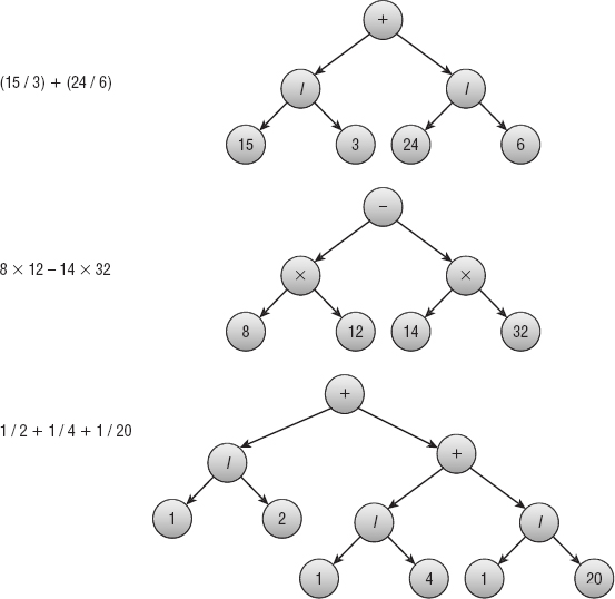
    Figure B-9: The expression trees on the right represent the expressions on the left.

23. Example program Expressions evaluates the necessary expressions.
24. Figure B-10 shows the expression trees.
25. Example program Expressions2 evaluates the necessary expressions.
26. Example program Quadtree demonstrates quadtrees.
27. Figure B-11 shows a trie for the given strings.

    

    Figure B-10: The expression trees on the right represent the expressions on the left.

    

    Figure B-11: This trie represents the strings APPLE, APP, BEAR, ANT, BAT, and APE.

28. Example program Trie builds and searches a trie.

Chapter 11: Balanced Trees

1. Figure B-12 shows the right-left rotation.
2. Figure B-13 shows an AVL tree as the values 1 through 8 are added in numeric order.
3. Figure B-14 shows the process of removing node 33 and rebalancing the tree. First you need to replace node 33 with the rightmost node to its left, which in this case is node 17. After that replacement, the tree is unbalanced at node 12, because its left subtree has height 2, and its right subtree has height 0. The tall grandchild subtree causing the imbalance consists of the node 8, so this is a left-right case. To rebalance the tree, you perform a left rotation to move node 8 up one level and node 5 down one level, followed by a right rotation to move node 8 up another level and node 12 down one level.

   

   Figure B-12: You can rebalance an AVL tree in the right-left case by using a right rotation followed by a left rotation.

   

   Figure B-13: An AVL tree remains balanced even if you add values in sorted order.

   

   Figure B-14: To rebalance the tree at the top, you need to replace value 33 with value 17, and then perform a left-right rotation.

4. Figure B-15 shows the process of adding the value 24 to the tree shown on the left.

   

   Figure B-15: When you add the value 24 to the tree on the left, the leaf containing values 22 and 23 splits.

5. Figure B-16 shows the process of removing the value 20 from the tree shown on the left. First, replace value 20 with value 13. That leaves the leaf that contained 13 empty. Rebalance by borrowing a value from a sibling node.

   

   Figure B-16: If you remove a value from a 2-3 tree node, and the node contains no values, you may be able to borrow a value from a sibling.

6. Figure B-17 shows the process of adding the value 56 to the B-tree on the top. To add the new value, you must split the bucket containing the values 52, 54, 55, and 58. You add the value 56 to those, make two new buckets, and send the middle value 55 up to the parent node. The parent node doesn't have room for another value, so you must split it too. Its values (including the new one) are 21, 35, 49, 55, and 60. You put 21 and 35 in new buckets and move the middle value 49 up to its parent. This is the root of the tree, so the tree grows one level taller.

   

   Figure B-17: Sometimes bucket splits cascade to the root of a B-tree, and the tree grows taller.

7. To remove the value 49 from the bottom tree in Figure B-17, simply replace the value 49 with the rightmost value to its left, which is 48. The node initially containing the value 48 still holds three values, so it doesn't need to be rebalanced. Figure B-18 shows the result.

   

   Figure B-18: Sometimes when you remove a value, no rebalancing is required.

8. Figure B-19 shows a B-tree growing incrementally as you add the values 1 through When you add 11, the root node has four children, so the tree holds 11 values at that point.

   

   Figure B-19: Adding 11 values to an empty B-tree of order 2 makes the root node hold four children.

9. A B-tree node of order K would occupy 1,024 × (2 × K) + 8 × (2 × K + 1) = 2,048 × K + 16 × K + 8 = 2,064 × K + 8 bytes. To fit in four blocks of 2 KB each, this must be less than or equal to 4 × 2 × 1,024 = 8,192 bytes, so 2,064 × K + 8 ≤ 8,192. Solving for K gives K ≤ (8,192 − 8) ÷ 2, 064, or K ≤ 3.97. K must be an integer, so you must round this down to 3.

   A B+tree node of order K would occupy 100 × (2 × K) + 8 × (2 × K + 1) = 200 × K + 16 × K + 8 = 216 × K + 8 bytes. To fit in four blocks of 2 KB each, this must be less than or equal to 4 × 2 × 1,024 = 8,192 bytes, so 216 × K + 8 ≤ 8,192. Solving for K gives K ≤ (8,192 − 8) ÷ 216, or K ≤ 37.9. K must be an integer, so you must round this down to 37.

   Each tree could have a height of at most log_(K+1)(10,000) while holding 10,000 items. For the B-tree, that value is log₄(10,000) ≈ 6.6, so the tree could be seven levels tall. For the B+tree, that value is log₃₈(10,000) ≈ 2.5, so the tree could be three levels tall.

Chapter 12: Decision Trees

1. Example program CountTicTacToeBoards does this. It found the following results:
   • X won 131,184 times.
   • O won 77,904 times.
   • The game ended in a tie 46,080 times.
   • The total number of possible games was 255,168.

   The numbers would favor player X if each player moved randomly, but because most nonbeginners have a strategy that forces a tie, a tie is the most common outcome.

2. Example program CountPrefilledBoards does this. Figure B-20 shows the number of possible games for each initial square taken. For example, 27,732 possible games start with X taking the upper-left corner on the first move.

   

   Figure B-20: These numbers show how many possible games begin with X taking the corresponding square in the first move.

   Because the tic-tac-toe board is symmetric, you don't really need to count the games from each starting position. All the corners give the same number of possible games, and all the middle squares also give the same number of possible games. You only really need to count the games for one corner, one middle, and the center to get all the values.

3. Example program TicTacToe does this.
4. Example program PartitionProblem does this.
5. Example program PartitionProblem does this.
6. Figure B-21 shows the two graphs. The graph of the logarithms of the nodes visited is almost a perfectly straight line for both algorithms, so the number of nodes visited by each algorithm is an exponential function of the number of weights N. In other words, if N is the number of weights, <Nodes Visited> = C^N for some C. The number of nodes visited is smaller for branch and bound than it is for exhaustive search, but it's still exponential.
7. Example program PartitionProblem does this.
8. Example program PartitionProblem does this.
9. The two groups are {9, 6, 7, 7, 6} and {7, 7, 7, 5, 5}. Their total weights are 35 and 31, so the difference is 4.
10. Example program PartitionProblem does this.

    

    Figure B-21: Because the graph of logarithm of nodes visited versus number of weights is a line, the number of nodes visited is exponential in the number of nodes.

11. The two groups are {5, 6, 7, 7, 7} and {5, 6, 7, 7, 9}. Their total weights are 32 and 34, so the difference is 2.
12. The two groups are {7, 9, 7, 5, 5} and {6, 7, 7, 7, 6}. Their total weights are both 33, so the difference is 0.
13. Example program PartitionProblem does this.

Chapter 13: Basic Network Algorithms

1. Example program NetworkMaker does this. Select the Add Node tool and then click on the drawing surface to create new nodes. When you select either of the add link tools, use the left mouse button to select the start node and use the right mouse button to select the destination node.
2. Example program NetworkMaker does this.
3. Example program NetworkMaker does this.
4. That algorithm doesn't work for directed networks because it assumes that if there is a path from node A to node B, there is a path from node B to node A. For example, suppose a network has three nodes connected in a row A → B → C. If the algorithm starts at node A, it reaches all three nodes, but if it starts at node B, it only finds nodes B and C. It would then incorrectly conclude that the network has two connected components {B, C} and {A}.
5. Example program NetworkMaker does this.
6. If the network has N nodes, any spanning tree contains exactly N − 1 links. If all the links have the same cost C, every spanning tree has a total cost of C × (N − 1).
7. Example program NetworkMaker does this.
8. Example program NetworkMaker does this.
9. No, a shortest-path tree need not be a minimal spanning tree. Figure B-22 shows a counterexample. The image on the left shows the original network, the middle image shows the shortest-path tree rooted at node A, and the image on the right shows the minimal spanning tree rooted at node A.

   

   Figure B-22: A shortest-path tree is a spanning tree but not necessarily a minimal spanning tree.

10. Example program NetworkMaker does this.
11. Example program NetworkMaker does this.
12. Example program NetworkMaker does this.
13. Example program NetworkMaker does this.
14. If the network contains a cycle with a negative total weight, the label-correcting algorithm enters an infinite loop following the cycle and lowering the distances to the nodes it contains.

    This cannot happen to the label-setting algorithm, because each node's distance is set exactly once and never changed.

15. After a node is labeled by a label-setting algorithm, its distance is never changed, so you can make the algorithm stop when it has labeled the destination donut shop. If the network is large and the start and end destination are close together, this change will probably save time.
16. When a label-correcting algorithm labels a node, that doesn't mean it will not later change that distance, so you cannot immediately conclude that the path to that node is the shortest, the way you can with a label-setting algorithm.

    However, the algorithm cannot improve a distance that is shorter than the distances provided by the links in the candidate list. That means you can periodically check the links in the list. If none of them leads to a distance less than the donut shop's distance, the donut shop's shortest path is final.

    This change is complicated and slow enough that it probably won't speed up the algorithm unless the network is very large and the start and destination nodes are very close together. You may be better off using a label-setting algorithm.

17. Instead of building a shortest-path tree rooted at the start node, you can build a shortest-path tree rooted at the destination node that uses the reverse of the network's links. Instead of showing the shortest path from the start node to every other node in the network, that tree will show the shortest path from every node in the network to the destination node. When construction makes you leave the current shortest path, the tree already shows the shortest path from your new location.
18. Example program NetworkMaker does this.
19. Example program NetworkMaker does this.
20. Building the arrays would take about 1 second for 100 nodes, 16.67 minutes for 1,000 nodes, and 11.57 days for 10,000 nodes.
21. Figure B-23 shows the Distance and Via arrays for the network shown in Figure 13-15. The initial shortest path from node A to node C is A → C with a cost of 18. The final shortest path is A → B → C with a cost of 16.

    

    Figure B-23: The Via and Distance arrays give the solutions to an all-pairs shortest-path problem.

Chapter 14: More Network Algorithms

1. Example program NetworkMaker does this.
2. When the algorithm adds a node to the output list, it updates its neighbors' NumBeforeMe counts. If a neighbor's count becomes 0, the algorithm adds the neighbor to the ready list. At that point, it could also add the neighbor to a list of nodes that are becoming available for work. For example, when the algorithm adds the Drywall node to the output list, the Wiring and Plumbing nodes both become ready, so they could be listed together. The result would be a list of tasks that become ready at the same time.
3. The algorithm should keep track of the time since the first task started. When it sets a node's NumAfterMe count to 0, it should set the node's start time to the current elapsed time. From that it can calculate the node's expected finish time. When it needs to remove a node from the ready list, it should select the node with the earliest expected finish time.
4. Yes. Just as at least one node must have out-degree 0 representing a task with no prerequisites, at least one node with in-degree 0 must represent a task that is not a prerequisite for any other task. You could add that task to the end of the full ordering. That would let you remove nodes from the network and add them to the beginning and end of the ordered list.

   Unfortunately, the algorithm doesn't have a good way to identify the nodes that have in-degree 0, so it would slow down the algorithm without some major revisions.

5. Example program NetworkMaker does this.
6. You could use the following pairs of nodes for nodes M and N: B/H, B/D, G/D, G/A, H/A, H/B, D/B, D/G, A/G, and A/H. Half of those are the same as the others reversed (for example, B/H and H/B), so there are really only five different possibilities.
7. Example program NetworkMaker does this.
8. Example program NetworkMaker does this. Run the program to see the four-coloring it finds.
9. Example program NetworkMaker does this. In my tests the program used five colors for the network shown in Figure 14-5 and three colors for the network shown in Figure 14-6. Run the program to see the colorings it finds.
10. The left side of Figure B-24 shows the residual capacity network for the network shown in Figure 14-12, with an augmenting path in bold. Using the path to update the network gives the new flows shown on the right. This is the best possible solution, because the total flow is 7, and that's all the flow that is possible out of source node A.

    

    Figure B-24: The augmenting path in the residual capacity network on the left leads to the revised network on the right.

11. Example program NetworkMaker does this. Load a network and select the Calculate Maximal Flows tool. Then left-click and right-click to select the source and sink nodes. Use the Options menu's Show Links Capacities command to show the link flows and capacities.
12. Figure B-25 shows example program NetworkMaker displaying maximal flows for the network shown in Figure 14-9. Only four jobs can be assigned. Load or create a work assignment network and select the Calculate Maximal Flows tool. Then left-click and right-click to select the source and sink nodes.

    

    Figure B-25: At most four jobs can be assigned in this work assignment network.

13. To find the number of paths that don't share links, simply give each link a capacity of 1, and find the maximal flow between the nodes. The total flow gives the number of paths.

    To find the number of paths that don't share links or nodes, replace each node with two nodes—an in-node and an out-node. Connect the two new nodes with a link of capacity 1. Make the links that entered the original node now enter the in-node. Make the links that exited the original node now exit the out-node. Now find the maximal flow. Because each original node is now represented by two nodes connected with a link of capacity 1, only one path can use each in-node/out-node pair.

14. You need only two colors to color a bipartite network. Simply give one color to one set of nodes and a second color to the other set of nodes. Because no link connects a node to another node in the same set, the two-coloring works.

    You can use three colors to color a work assignment network. Use one color for the employee nodes, one color for the job nodes, and one color for the source and sink nodes.

15. Example program NetworkMaker does this. Load a network and select the Minimal Flow Cut tool. Then left-click and right-click to select the source and sink nodes.
16. There are two solutions. The first solution removes links B → C, E → F, and H → I. The second solution removes links C → F, E → F, and H → I. Both solutions remove a total capacity of 7. Example program NetworkMaker finds the first of these two solutions.

Chapter 15: String Algorithms

1. Example program ParenthesisMatching does this.
2. Example program EvaluateExpression does this.
3. The program would need to look for a fourth recursive case in which the expression is of the form -expr for some other expression expr.
4. The program would need to look for another recursive case in which the expression is of the form Sine(expr) for some other expression expr.
5. Example program EvaluateBoolean does this.
6. Example program GraphExpression does this.
7. Table B-3 shows a state transition table for a DFA that matches the regular expression (AB)*|(BA)*.

   Table B-3: A State Transition Table for (AB)*|(BA)*.

   

8. Figure B-26 shows the state transition diagram.

   

   Figure B-26: This DFA state transition diagram matches the regular expression ((AB)|(BA))*.

9. Table B-4 shows a state transition table for the state transition diagram shown in Figure B-26.

   Table B-4: A State Transition Table for ((AB)|(BA))*.

   

10. Example program DFAMatch does this.
11. A table is easy to write down, but it's not easy to look up transitions when you need them. For example, suppose the DFA is in state 17, and it sees the input H. The program would need to search the table to find the appropriate entry before moving to the new state. If the table is large, this could take a while. To speed things up, you might store the transitions in a tree, hash table, or some other data structure to make finding transitions easier. That would take up more memory and complicate the program.

    In contrast, suppose you use objects to represent the states, similar to how you can use node objects to represent locations in a network. Each state object could have a list giving the new state object for various inputs. In that case, state transitions would be relatively quick and simple. If some states can read many possible inputs (in other words, there are many links leaving them in the state diagram), you might still spend some time looking up new states. In that case you might want to use a tree, hash table, or some other data structure to make finding the new states faster, but at least you won't have to search the whole transition table.

12. Build the NFA states as usual to recognize the pattern. Then add a new start state at the beginning. Add a null transition that connects the new state to the normal states. Add another transition that connects the new start state to itself on every input character. Finally add a transition that connects the pattern's accepting state to itself on any input character. Figure B-27 shows the transition diagram.

    

    Figure B-27: This NFA state transition diagram matches a pattern anywhere within a string.

13. Figure B-28 shows the solution.

    

    Figure B-28: The parse tree (left) and corresponding NFA network (right) for the expression (AB*)|(BA*).

14. Figure B-29 shows the solution.

    

    Figure B-29: This DFA state transition diagram matches the same values as the NFA state transition diagram shown on the right in Figure B-28.

15. Let the target consist of a series of A's and the text consist of runs of M − 1 A's followed by a B. For example, if M is 4, then the target is AAAA, and the text is AAAB repeated any number of times. In this case, the target is not present in the text, because there are never M A's in a row. As the outer loop variable i changes, the inner loop must run over M, M − 1, M − 2, ..., 1 values to decide that it has not found a match. Then the sequence repeats. On average, the inner loop runs roughly M / 2 times, giving a total run time of O(N × M / 2) = O(N × M).
16. The least-cost path uses as many diagonal links as possible. In Figure 15-13, a path can use at most four diagonal links. A path that uses four diagonal links uses five nondiagonal links, so the edit distance is 5.
17. Example program StringEditDistance does this.
18. Example program StringEditDistance does this.
19. Yes, the edit distance is commutative. To transform word 2 into word 1, you can reverse operations. In other words, instead of deleting a character, insert one, and instead of inserting a character, delete one.
20. Example program FileEditDistance does this.
21. Example program FileEditDistance does this.

Chapter 16: Encryption

1. Example program RowColumnTransposition does this.
2. Example program SwapColumns does this.
3. If the key contains duplicated characters, there's no way to know which of the corresponding columns should come first.

   One solution is to use only the first occurrence of each letter, so PIZZA becomes PIZA and BOOKWORM becomes BOKWRM. This actually has the small benefit of increasing obscurity if the attacker doesn't know the rule, because it disguises the number of columns in the encryption array.

4. Swapping both columns and rows greatly increases the number of possible arrangements of rows and columns. For example, if a message contains 100 characters and is written into a 10×10 array, there are 10! × 10! ≈ 1.3×10¹³ possible arrangements of the rows and columns.

   However, if the attacker figures out only the column ordering, the rows will be out of order, but each row in the array will contain valid words. By recognizing the valid words, the attacker can recover the column ordering and then try to swap rows to recover the full message.

   If each row begins with a new word, finding the row ordering could be difficult. But if words span rows, the pieces of the words will give the attacker extra clues for finding the row ordering. For example, suppose the first row ends with GREA, the second row begins with NT, and the third row begins with TLY. In that case, it's likely that the third row should follow the first row.

   This is an example in which what seems like a perfectly reasonable attempt to add one encryption method to another doesn't really help much. Although adding row transpositions to column transpositions greatly increases the number of possible combinations, it doesn't greatly increase the number of combinations the attacker must consider.

5. Example program SwapRowsAndColumns does this.
6. Example program CaesarSubstitution does this. The encryption of “Nothing but gibberish” with a shift of 13 is ABGUV ATOHG TVOOR EVFU.
7. Example program LetterFrequencies displays the relative frequencies of the letters in a message. That program finds the following values for the three most common letters in the ciphertext:

   

   Using the CaesarSubstitution example program with offset 6 to decipher the message produces gibberish. Using the program again with offset 17 gives the plain-text message THERE WASAT IMEWH ENCAE SARSU BSTIT UTION WASTH ESTAT EOFTH EART. (There was a time when Caesar substitution was the state of the art.)

8. Example program VigenereCipher does this. The decrypted message is AVIGE NEREC IPHER ISMOR ECOMP LICAT EDTHA NCAES ARSUB STITU TION. (A Vigenère cipher is more complicated than Caesar substitution.)
9. If you reuse a one-time pad, you are essentially using a Vigenère cipher where the keyword is the entire pad. You might get away with this for a little while, but eventually, if the attacker knows that you are reusing the pad, the cipher may be broken.
10. This would happen if a message was lost or you received messages out of order so that you're not using the right letters in the pad. You can decrypt the message by starting at different positions in the pad until you find a position that produces a readable message. The number of letters in the pad that you needed to skip tells you how long the message was that you missed. You can either ignore that message or give the sender a message (encrypted, of course) asking for the missing message to be repeated.
11. Not much. It would give the attacker information about the length and frequency of the messages you are sending, but the attacker can learn that anyway by looking at the lengths of intercepted messages (assuming that all messages are intercepted).
12. Example program OneTimePad does this.
13. If you have a cryptographically secure random-number generator, you can use it to generate one-time pads and use those for encryption. A one-time pad is unbreakable because any message letter could become any ciphertext letter.

    Conversely, suppose you have an unbreakable encryption scheme. You could use it to encrypt a message consisting of nothing but instances of the letter A to generate a sequence of random letters. You could then use those letters to generate the random numbers for a secure random-number generator.

14. Always send a message of the same length at the same time every day. If you have nothing to say, just say that. Pad the messages to the same length with random characters. If the encryption is secure, the attacker cannot tell when a message contains important information and when it contains random characters.
15. For this scenario, the answers are as follows:

    

Chapter 17: Complexity Theory

1. Countingsort and bucketsort don't use comparisons. Instead, they perform mathematical calculations to find where in the sorted list each value should go.
2. This can be reduced to the two-coloring problem. If the graph is two-colorable, it is bipartite. To use a two-coloring algorithm to solve the bipartite detection problem, try to two-color the graph. If a two-coloring is possible, the graph is bipartite. The two-coloring even gives you the two node sets for the bipartite graph. Just put nodes with one color in one set and nodes with the other color in the other set.

   The two-coloring algorithm described in Chapter 14 runs in polynomial time (actually, it's quite fast), so it's in P, and the bipartite detection is also in P.

3. The three-cycle problem can be reduced to the bipartite detection problem. If a graph has a cycle of length 3, it is not bipartite. To solve the three-cycle problem, use a bipartite detection algorithm to see if the graph is bipartite. If the graph is bipartite, it does not contain any cycles of length 3.

   Note that the converse is not necessarily true. If the graph has no cycles of length 3, it is still not bipartite if it has a cycle with an odd length.

   Exercise 2 shows that the bipartite detection problem is in P, so the three-cycle problem is also in P.

4. The odd-cycle problem also can be reduced to the bipartite detection problem. If a graph has a cycle with odd length, it is not bipartite. To solve the odd-cycle problem, use a bipartite detection algorithm to see if the graph is bipartite. If the graph is bipartite, it does not contain any cycles of odd length.

   Note that for this case, the converse is also true. If the graph has no cycles of odd length, it is bipartite.

   Exercise 2 shows that the bipartite detection problem is in P, so the odd-cycle problem is also in P.

5. A nondeterministic algorithm for solving HAM is as follows: Guess the order in which the nodes can be visited, and then verify (in polynomial time) that the ordering gives a Hamiltonian path. To do that, you need to verify that every node is in the ordering exactly once and that there is a link between the adjacent pairs of nodes in the ordering.
6. You can use a nondeterministic algorithm similar to the one described in the solution to Exercise 5: Guess the order in which the nodes can be visited, and then verify (in polynomial time) that the ordering gives a Hamiltonian cycle. The only difference is that for this problem you also need to verify that the first and last nodes are the same.
7. HAM and HAMC are very closely related, but they don't instantly solve each other, because a network can contain a Hamiltonian path without containing a Hamiltonian cycle. (For example, consider a two-node network with a single link A → B. The ordering A → B gives a Hamiltonian path but not a Hamiltonian cycle.)

   To reduce HAM to HAMC, you must find a way to use a HAMC algorithm to solve HAM problems. In other words, if a network contains a Hamiltonian path, you must use a HAMC algorithm to detect it.

   First, note that a network that contains a Hamiltonian cycle contains a Hamiltonian path. Simply take a Hamiltonian cycle and remove the final link to form a Hamiltonian path.

   Now suppose the network doesn't contain a Hamiltonian cycle, and suppose it does contain a Hamiltonian path. How could you turn the path into a cycle? Simply add the path's starting node to the end of the path. If a link from the ending node to the starting node was already in the network, it would have already contained a Hamiltonian cycle, so that link must not be present.

   To look for a Hamiltonian cycle, add a new link L_ABbetween two nodes A and B. Now if there is a Hamiltonian cycle, the same ordering gives you a Hamiltonian path in the original network. Suppose the Hamiltonian cycle passes through the nodes N₁, N₂, ..., A, B, N_k, N_k+1, ... N₁. Then the original network contains the Hamiltonian path B, N_k, N_k+1, ... N₁, N₂, ..., A.

   The complete algorithm for solving HAM is as follows:

   1. Use the HAMC algorithm to see if the original network contains a Hamiltonian cycle. If it does, it contains a Hamiltonian path.
   2. For every pair of nodes A and B, if there is not already a link from node A to node B:
      1. Add a link LAB between nodes A and B.
      2. Use the HAMC algorithm to see if the modified network contains a Hamiltonian cycle. If it does, the original network contains a Hamiltonian path.
      3. Remove link LAB, and continue trying other pairs of nodes.

   Figure B-30 shows the idea. The original network is on the left. This network clearly has no Hamiltonian cycle, because node L has only one link, so a path that enters that node cannot leave it again.

   

   Figure B-30: The network on the left contains a Hamiltonian path but no Hamiltonian cycle.

   As the reduction algorithm progresses, it eventually tries adding a link between nodes I and L. The HAMC algorithm finds the Hamiltonian path shown on the right in Figure B-30. If you remove the link between nodes I and L, you get a Hamiltonian path in the original network.

   Note that this may be an inefficient algorithm for finding Hamiltonian paths. If the network contains N nodes, you may need to repeat Step 2 up to N² times. That's still polynomial time, however, so this is a polynomial time reduction.

   The HAMC algorithm is NP-complete so it has no known fast solutions. That means running it N² times will be very slow indeed.

8. To reduce HAMC to HAM, you must find a way to use a HAM algorithm to solve HAMC problems. In other words, if a network contains a Hamiltonian cycle, you must use a HAM algorithm to detect it.

   Unfortunately, you can extend a Hamiltonian path to form a cycle only if the last node in the path has a link leading to the first node in the path. A HAM algorithm might find a path that does not have such a link, so it could not form a cycle.

   Suppose the network contains a Hamiltonian cycle that includes the link L_AB connecting nodes A and B. Now suppose you connect a new node A' to node A and a new node B' to node B. Then the new network contains a noncyclic Hamiltonian path starting at node A' and ending at node B'.

   Conversely, any Hamiltonian path must start at node A' and end at node B' (or vice versa in an undirected network). Suppose the HAM algorithm finds a path that visits the nodes A', A, N₁, N₂, ..., B, B'. Then the path A, N₁, N₂, ..., B, A is a Hamiltonian cycle.

   The complete algorithm for solving HAMC is as follows:

   1. For every link LAB connecting nodes A and B:
      1. Connect a new node A' to node A, and connect a new node B' to node B.
      2. Use the HAM algorithm to see if the modified network contains a Hamiltonian path. If it does, the original network contains a Hamiltonian cycle.
      3. Remove the new nodes A' and B' and the links connected to them, and continue with another link.

   Figure B-31 shows the idea. You can probably find a Hamiltonian cycle easily enough, but pretend you can't. In the image on the right, the reduction algorithm is considering the link L_QR connecting nodes Q and R. It has added node Q', connected to node Q, and node R', connected to node R. The Hamiltonian path algorithm finds the path shown in bold in the modified network on the right. Removing the Q' and R' nodes and their links and adding the L_QR link to the path gives a Hamiltonian cycle.

   

   Figure B-31: The bold Hamiltonian path in the network on the right corresponds to a Hamiltonian cycle in the network on the left.

9. The nondeterministic algorithm is as follows: Guess the coloring. For each node, verify that its neighbors have a different color from the node.
10. The nondeterministic algorithm is as follows: Guess the subset. Then add up the numbers and verify that their total is 0.
11. The following pseudocode shows one way to reduce the reporting problem to the detection algorithm:
    1. If DetectKnapsack(k) returns false, no subset with a value of at least k will fit in the knapsack, so the reporting algorithm can return that information and stop.
    2. If DetectKnapsack(k) returns true, for each object Oi in the set:
       1. Remove object Oi from the set.
       2. Use DetectKnapsack(k) to see if a solution with value k is still possible.
       3. If a solution with value k is still possible, leave out object Oi, and continue the loop in Step 2.
       4. If a solution with value k is no longer possible, restore object Oi to the set, and continue the loop in Step 2.

    When the loop has finished, the items that are still in the set form the solution.

12. The following pseudocode shows one way to reduce the optimization problem to the detection algorithm:
    1. Suppose Kall is the total value of all the objects in the set. Use the detection algorithm DetectKnapsack(Kall), DetectKnapsack(Kall − 1), DetectKnapsack(Kall − 2), and so on until DetectKnapsack(Kall − m) returns true. At that point, Kall − m is the maximum possible value that you can fit in the knapsack. Let Kmax = Kall − m.
    2. Use the reduction described in the solution to Exercise 11 to find ReportKnapsack(Kmax). The result is the result of the optimization problem.
13. The following pseudocode shows one way to reduce the reporting problem to the detection algorithm:
    1. If DetectPartition() returns false, no even division is possible, so the reporting algorithm can return that information and stop.
    2. If DetectPartition() returns true:
       1. Let Omax be the object with the greatest value, and assume Omax is in Subset A. (If a partitioning is possible, it is possible with Omax in Subset A. If you find a partitioning and Omax in Subset B, just swap every item between the two subsets.)
       2. For each of the other objects Oi:
          1. Remove Oi from the set, and add its value Vi to the value of object Omax.
          2. Use the DetectPartition algorithm to see if a partitioning is still possible. If it is, a partitioning of the original set is possible with Oi in Subset A. Leave the set and Vmax as they currently are, and continue the loop in Step 2b.
          3. If DetectPartition indicates that a partitioning is no longer possible, object Oi must be placed in Subset B. In that case, subtract the Vi you added to Vmax, and add Oi back into the set to restore the set to the way it was before Step 2b-ii. To represent putting Oi in Subset B, remove object Oi from the set, and subtract its value Vi from Vmax. Now continue the loop in Step 2b.

    When the loop in Step 2b has finished, the set should contain only Omax, and Vmax should be 0. The steps you took to get there tell you which items belong in Subset A and which belong in Subset B.

Chapter 18: Distributed Algorithms

1. Figure B-32 shows the zero-time sort algorithm sorting the two lists.

   

   Figure B-32: A systolic array of four cells can sort two lists containing four numbers each in a total of 15 ticks.

   Sorting two lists of numbers takes only one tick longer than sorting a single list.

2. Suppose the shared best route length is 100, and process A has a new route with a total length of 80. It reads the shared value and enters its If Then block. Now process B compares the shared value to its new route length of 70, so it also enters its If Then block, and it acquires the mutex first. Process B saves its solution, along with the new total route length of 70, and releases the mutex. Now process A acquires the mutex and saves its solution with the total route length 80.

   In this case, the solution saved by process A is worse than the one saved by process B. The route length saved by process A matches the solution saved by process A, so this is a little better than the original race condition example, but the best solution is still overwritten. Process B also has a local copy of what it thinks is the best route length, 70, so it would not report a new solution with a route length of 70 if it found one.

   Process A can save itself if it checks the shared route length again after it acquires the mutex. You can void that extra step if you acquire the mutex first, but there may actually be a benefit to checking the value twice.

   Acquiring a mutex can be a relatively slow operation, at least compared to checking a memory location. If process A's value isn't as good as the value already stored in the shared variable, process A can learn that quickly and not bother acquiring the mutex.

3. Figure B-33 shows the situation for four philosophers. Forks with a line through them are dirty. The image on the left shows the initial situation, in which philosopher 4 has no forks, philosopher 1 has two forks, and the other philosophers hold their left forks.

   

   Figure B-33: In the Chandy/Misra solution with synchronized philosophers, philosopher 1 eats first, and philosopher N eats second.

   When the philosophers all try to eat at the same time, philosopher 1 already has two forks, so he succeeds and is the first to eat. The others (except for philosopher 4) already hold dirty left forks, so they request right forks. Philosopher N has no forks, so he requests both forks. Because all the forks are dirty, those who have them clean their left forks and give them away (except philosopher 1, who is eating). The result is shown in the middle of Figure B-33.

   In this example, two of the philosophers now have a clean right fork and no left fork, so they ask for the left fork. (In a large problem, most of the philosophers would have a clean right fork and no left fork.) Their neighbors hold clean forks, so they refuse to give them up, and everyone waits.

   When philosopher 1 finishes eating, he cleans his forks and gives them to his neighbors, philosophers 2 and 4. The result is shown on the right in Figure B-33. Philosopher 4 now has two forks, so he is the second to eat.

   When philosopher 4 finishes eating, he gives his right fork to philosopher 3, who then eats.

   When philosopher 3 finishes eating, he gives his right fork to philosopher 2, who then eats last.

   More generally, the philosophers eat in the order 1, N, N − 1, N − 2, ..., 2.

4. In that case, general A never receives an acknowledgment. Therefore, he assumes he didn't send enough messages the first time around, and he sends another batch with more messages. General B receives some of those messages and sends a new batch of acknowledgments (possibly including more this time). Eventually the generals will go through enough rounds that general A will receive an acknowledgment.
5. General A sends a batch of messages as before. If general B receives any messages, he calculates P_AB and then sends a batch of 10 acknowledgments that say, “P_AB = <calculated value>. This is acknowledgment 1 of 10. I agree to attack at dawn.”

   If general A receives any acknowledgments, he calculates P_BA. The content of the acknowledgments tells him P_AB. He uses P_AB to decide how many messages to send to get a desired level of certainty, and he sends messages saying, “P_BA = <calculated value>. Acknowledgment received.”

   After the first batch of messages, if general A doesn't receive any acknowledgments (when he sent them, he didn't know P_AB, so he didn't know how many to send), he assumes general B didn't receive any. So he sends another, larger batch.

   Similarly, if general B doesn't receive a reply to the acknowledgments (when he sent them, he didn't know P_BA, so he didn't know how many to send), he assumes general A didn't receive any. So he sends another, larger batch.

   Eventually general A will send enough messages for general B to receive some and calculate P_AB. After that, general B will eventually send enough acknowledgments for general A to receive some and calculate P_BA. Finally, general A will eventually send enough replies to give general B the value P_BA, and both generals will know both probabilities.

6. That would work in the situation shown on the right of Figure 18-2.

   In the situation shown on the left of Figure 18-2, however, each lieutenant makes a decision. In some sense it doesn't matter what each does, because the general is a traitor, and there's no rule that they need to obey a traitorous general. However, there is a rule that two loyal lieutenants must decide on the same action, and in this case they don't.

7. That would work in both of the situations shown in Figure 18-2. In both situations, the lieutenants receive conflicting instructions, so they both retreat.

   However, suppose the general is loyal (as in the situation on the right of Figure 18-2). The general orders an attack, and the traitorous lieutenant on the right lies about it. In that case, the lieutenant on the left receives conflicting orders, so he retreats, violating the general's orders.

8. No, there isn't enough information for the loyal lieutenants to identify the traitor. For example, consider two scenarios. First, suppose the general is a traitor who tells the first lieutenant to attack and the other lieutenants to retreat. After the lieutenants exchange information, they believe they were all told to retreat, except for the first lieutenant.

   For the second scenario, suppose the first lieutenant is a traitor. The general tells all the lieutenants to retreat, but the traitor tells the others that the general told him to attack.

   The lieutenants receive the same information in both scenarios, so they cannot tell whether the traitor is the general or the first lieutenant.

   These two scenarios hold no matter how many lieutenants there are, so there is no way to identify the traitor.

   (The traitor could also simply act as if he is loyal and not give conflicting orders. Then there is no way to detect him, although he won't cause any harm that way either.)

9. Suppose the general tells two lieutenants to attack and two to retreat. After exchanging orders, the lieutenants all believe two attack orders and two retreat orders were given. A single traitor lieutenant could not create that set of orders, so the traitor must be the general.

   If this occurs, the lieutenants don't need to obey the traitor, but they still need to agree on a common decision. They can do that with a predefined rule that says, “If the commanding general is a traitor, retreat.”

10. The dining philosophers problem assumes that the philosophers cannot talk to each other. If you let them talk, they can elect a leader who can act as a waiter.
11. A bully algorithm would let a philosopher remove a fork from a philosopher who has a lower ID. That would help if the philosophers don't eat too often. But if they eat a large percentage of the time, this might lead to a livelock in which philosophers with lower IDs don't get to eat very often.
12. If the philosophers want to eat too often, they probably will waste a lot of time waiting for forks. A waiter who allows all odd-numbered philosophers to eat at the same time and then allows all even-numbered philosophers to eat at the same time would be much more efficient than a free-for-all.
13. Suppose D_AB and D_BA are the delays for sending a message from A to B and B to A, respectively, and consider the equations the algorithm uses to calculate the clock error:

    

    Now, if you subtract the second equation from the first, you get this:

    

    In the previous analysis where D_AB = D_BA, those two terms cancel. If you leave the terms in the equation and solve for E, you get this:

    

    The error in E due to the difference between D_BA and D_AB is half of their difference. In the worst case, where one of these is close to 0 and the other is close to the total roundtrip delay D, the error is D ÷ 2.

    After running the clock algorithm, T_B = T_A ± D ÷ 2.

14. There really isn't any difference between the network speed's changing and it taking a different amount of time for a message to go from A to B or from B to A. In either case, all that matters is that the values D_BA and D_AB from the answer to Exercise 13 are different. That answer shows that after the clock algorithm runs, T_B = T_A ± D ÷ 2, where D is the total delay.
15. The answer to Exercise 14 shows that the error in process B's new time is determined by the total roundtrip message delay D. If the network's speed varies widely, sometimes D will be short, and sometimes D will be long. To get a better result, perform the algorithm several times, and adjust the time according to the trial with the smallest value for D.

Chapter 19: Interview Puzzles

1. If he brings three socks into the living room, they can't all three be different colors, so at least two will be either brown or black.

   This problem is simple if you have seen a similar problem before, so it doesn't really test the reasoning ability of anyone who has seen something similar. It's also easy if you write down some possible combinations. Overall it's not too bad a question, but it doesn't really tell the interviewer much.

2. If you put all the marbles in one bowl, or put half of each color in each bowl, you have a 50% chance of picking a white marble, so that's a quick lower bound for the possible probability. Similarly if you put all of the white marbles in one bowl and all of the black marbles in the other bowl, you have a 50% chance of picking a white marble.

   A better solution is to put a single white marble in one bowl and all the other marbles in the other bowl. When you pick a marble, there is a 50% chance that you'll get lucky and pick the bowl that holds the single white marble. If you're unlucky and pick the other bowl, there's still a 9 in 19 chance that you'll get lucky and pick a white marble. Your total odds are as follows:

   

   This problem involves a little probability but is mostly a clever trick. It would be easier, quicker, and potentially less frustrating to ask the candidate how much he or she knows about probability.

3. At first this seems like a probability or counting question, but it's actually a trick question. There aren't enough red marbles to place one between each pair of blue marbles, so it would be impossible to do so.

   This problem is easy if you get the trick, but if you don't, you may waste a lot of time on it. In either case, the interviewer doesn't learn much about the candidate.

4. This is really a counting question. You can find the probability by dividing the number of “good” arrangements by the number of total arrangements.

   First, notice that you don't need to consider arrangements in which you swap marbles of the same color. All red marbles are the same, and all blue marbles are the same.

   Next, to simplify the procedure, assume you have straightened out the circle of marbles so that you have a row of 12 slots where a marble can be positioned. Now place a blue marble in the first slot. Positioning the other 11 marbles in the remaining 11 slots is equivalent to positioning the original 12 marbles in 12 slots arranged in a circle. This situation is easier to handle because you don't need to worry about the effects of the arrangement wrapping around the circle so that the first marble is adjacent to the last marble. Now a blue marble separates the first and last red marbles.

   Now you can think of the problem as having 11 slots where you will place the remaining 11 marbles. If you pick slots for the four red marbles, the blue ones will fill in the remaining empty slots. If you think of it this way, the number of possible arrangements is as follows:

   

   To see how many “good” arrangements are possible, start by placing the four red marbles in a row. To ensure that no two red marbles are adjacent, you must put three of the seven remaining blue marbles between each pair of red marbles.

   At this point, four blue marbles are left, and they can go anywhere. If you think of the red marbles as defining walls, the remaining blue marbles must go between the walls. (It doesn't matter how the marbles between the walls are ordered, because you can't tell the blue marbles apart.)

   One way to think about this is to imagine eight slots where you will put either a blue marble or a wall. Now you can pick slots for the walls and fill in the remaining slots with blue marbles. The number of ways you can do that is as follows:

   

   The number of “good” arrangements is 70, and the total number of possible arrangements is 330, so the odds that a random arrangement is “good” are 70 ÷ 330 = 7/33 ≈ 21%.

   This problem is pretty interesting, but it's quite difficult. This kind of problem is fairly common in probability and statistics courses, so a candidate who has taken such a course will probably know the basic approach. Even then it would be a tough calculation, and if the candidate hasn't taken that kind of course, this problem will be extremely hard.

   All that the interviewer will really learn from this question is whether the candidate has seen a problem like this before or has taken such a course.

5. The most obvious approach is to use a linked list. You could also do this in an array with a For loop. You get bonus points if you mention both methods and say that the better method depends on how the list is already stored for use in performing other operations.

   This is actually a relevant question! You may never need to reverse a list of customers in this way, but answering this question shows that you know about at least one type of data structure. Mentioning both the linked list and array solutions shows you know about at least two data structures and that you can look for more solutions even after you find one.

6. This problem has a couple good approaches. For the algebraic approach, let M be my current age, and let B be my brother's current age. Then:

   

   Plugging the first equation into the second gives you this:

   

   Rearranging and solving for B gives you this:

   

   Inserting this value into the first equation gives M = 3 × 2 = 6, so I am 6 right now.

   A second approach is to make a table similar to the following, starting with a guess of age 30 for yourself:

   

   After filling in the first row, you compare the last two columns. In this case, My Age + 2 is too big, so you guess again with smaller ages:

   

   In the second row, the difference between the last two columns is closer but still is too big, so you guess again with even smaller ages:

   

   In this example, the third row finds the solution. (If you overshoot and My Age + 2 turns out too small, try larger ages.)

   This problem is almost worth asking because it lets you see whether the candidate is more comfortable using algebra or a table. I'm not sure how useful that information will be, though. Many problems like this one are more involved, so a table won't work well, but just because the candidate used a table doesn't mean he or she can't use algebra if it's required.

   If you use a problem like this, it's probably best to ask the candidate why he or she chose a particular approach and what other approaches might also work.

7. This problem is somewhat relevant for programmers because it involves a “fencepost problem.” Suppose you're building a fence with rails between posts. There will be one more post than rails, because you need a post on each end of the fence. A fencepost problem (or off-by-1 problem) occurs when a programmer accidentally counts some object one too many times or one too few times.

   For this problem, the minute hand passes the hour hand a bit after 1:05, a bit longer after 2:10, and so on up to some time after 10:50. The next time the hands meet after 11:00 is 12:00 midnight. That means the hands cross between 1:00 and 2:00, between 2:00 and 3:00, and so on up to a time between 10:00 and 11:00. (At this point, perhaps you can see the fencepost problem.)

   If you only count times strictly between noon and midnight, the hands cross 10 times. If you also count the times they cross at noon and midnight, the hands cross 12 times.

   How the candidate approaches this question may tell you a bit about how methodical he or she is, but that may be all it tells you. At least a careful candidate can come up with some solution either right or wrong without knowing a sneaky trick.

8. (Microsoft has used this question in interviews.) The following paragraphs describe three ways to look at this problem:
   1. A short, off-the-cuff answer is “50%, because boys and girls are equally likely, so in any given population of children, 50% are girls.” That's a good “big picture” answer, but it's not necessarily very intuitive, so the interviewer might ask you to prove it. (That answer actually does prove it, but digging in at this point will probably just annoy the interviewer.)
   2. Another slightly more intuitive way to look at this problem is to consider first children, second children, third children, and so on. All the couples have at least one child. Half of those are boys, and half are girls, so the population of first children is half boys and half girls.

      The couples whose first child is a girl have a second child. Of those children, half are boys and half are girls, so the population of second children is half boys and half girls.

      The couples whose first and second children are girls have a third child. Of those children, half are boys and half are girls, so the population of third children is half boys and half girls.

      At this point it should be clear that each cohort is half boys and half girls, so the population as a whole must be half boys and half girls.

   3. For a third way to look at the problem, consider a couple's first child. There's a 50% chance it is a boy, and they stop having children, but there's a 50% chance that they have a girl. After one child, their expected number of children is 0.5 boys and 0.5 girls.

      If the couple's first child is a girl, they have a second child. Again, there's a 50% chance of a girl and a 50% chance of a boy. The expected contribution to the family of this child is the chance of having a second child in the first place (0.5) times the chance of having a boy or a girl. That adds another 0.5 × 0.5 = 0.25 expected boys and 0.5 × 0.5 = 0.25 expected girls to the family, making a total expected 0.75 boys and 0.75 girls.

      Hopefully at this point you can see a pattern.

      In general, to have an Nth child, the couple must previously have had N − 1 girls in a row. The chance of that happening is 1/2^N–1.

      Assuming they did have N − 1 girls in a row, there is a 50% chance that the next child is a boy and a 50% chance that the next child is a girl. Therefore, the expected contribution to the family of the Nth child is 0.5 × 1/2^N–1 = 1/2^N boys and 0.5 × 1/2^N = 1/2^N girls.

      If you add up the expected number of children through child N, you get the following:

      

      These values are the same. Each couple has the same expected number of boys and girls, and so does the population as a whole.

      If you take the limits of these sums as N goes to infinity, these equations also show that the expected number of children for each family is one boy and one girl.

   This is an interesting problem, but it's fairly easy if you've seen it before and rather tricky if you haven't. (In the real world, the chances of having a boy or girl are not exactly 50% and even depend on the ages of the parents. For more information, see the Psychology Today article “Why Are Older Parents More Likely to Have Daughters” at http://www.psychologytoday.com/blog/the-scientific-fundamentalist/201104/why-are-older-parents-more-likely-have-daughters.)

9. Don't make the interviewer mad by pointing out that this is an unrealistic situation. The question basically asks you to cut the brick into pieces so that you can make combinations that add up to 1/7th, 2/7ths, 3/7ths, 4/7ths, 5/7ths, 6/7ths or the whole brick.

   Clearly you could cut the brick into seven pieces and hand out one for each day worked.

   There are several ways you can arrive at the best solution. In one approach, you consider how you can pay the contractor after each possible ending day.

   If the job ends after one day, you must give the contractor 1/7th of the brick, so clearly you need a piece that is 1/7th of the brick.

   If the job ends after two days, you must give the contractor 2/7ths of the brick. You could give him another 1/7th piece, but that won't give you any extra flexibility later. A better solution is to give him a piece that is 2/7ths of the brick and keep the 1/7th piece.

   Because you have the 1/7th piece in reserve, you can use it and the 2/7ths piece to pay the contractor if the job ends after three days. If you had used two 1/7th pieces to pay the contractor after two days, this solution wouldn't work. You would need a third 1/7th piece so you would need to have three pieces instead of just two.

   If you remove two pieces from the brick that are 1/7th and 2/7ths of the whole brick, the remaining brick contains 4/7th of the brick. If the job ends after four days, you can give the contractor that piece and keep the others.

   If the job ends after five days, you can give the contractor the 4/7ths piece and the 1/7th piece.

   If the job ends after six days, you can give the contractor the 4/7ths piece and the 2/7ths piece.

   Finally if the job ends after seven days, you can give the contractor all the pieces.

   When a problem involves magic numbers such as powers of 2 or 1 less than a power of 2, you should think about binary. In this example, the three pieces of the brick represent 1, 2, and 4 sevenths of the brick. The numbers 1 through 7, which are 001, 010, 011, 100, 101, 110, and 111 in binary, tell you which pieces of the brick to give to the contractor on each day. A 1 means you should give the contractor the corresponding piece, and a 0 means you should keep that piece.

   For example, 6 is 110 in binary. That means on day 6 you give the contractor the 4/7ths piece (for the initial 1) and the 2/7ths piece (for the second 1) but not the 1/7th piece (for the final 0). The total payment on that day is 4/7 + 2/7 = 6/7.

   This problem is easy if you've seen it before and can be confusing if you haven't, although you probably can come up with a solution if you work through it starting from day 1. Being aware of magic numbers can help.

10. This is one of a large family of pan balance puzzles. Whenever you have a tool such as a pan balance that divides a collection of objects into sets, you should think about a subdivision approach. If you can divide a set of objects into two groups and eliminate one group from consideration at each step, you can use a binary subdivision approach to find whatever you're looking for.

    In this problem, that doesn't quite work. If you put four eggs on each side of the balance, you can eliminate half of the eggs from consideration in one weighing. Then you can place the remaining four eggs, two on each side of the balance, and eliminate two more from consideration. At that point, you're still left with two eggs, and you've used up your two weighings.

    The key to this problem is noticing that the balance doesn't define only two sets containing eggs in the left pan and eggs in the right pan. It also defines a third set containing eggs that are not in either pan. Instead of using binary division to divide the eggs into two groups and eliminating one, you can use ternary division to divide the eggs into three groups and eliminate two.

    Suppose you have only three eggs. You could put one in the left pan, one in the right, and omit one. If the two pans balance, you know the third egg is goldplated. If the two pans don't balance, you know the egg in the lighter pan is the gold-plated egg.

    That explains how you perform the second weighing to finalize your choice. You still need to figure out how to use the first weighing to reduce the number of remaining eggs to three (or fewer).

    The balance lets you eliminate two of the three groups. After one weighing, the set of eggs still under consideration must include only three eggs. That means the groups you weigh in the first weighing should contain three eggs each.

    Here's the final solution:

    1. Place three eggs in the left pan, three in the right, and omit two.
    2. If the pans balance:
       1. The gold-plated egg is one of the two eggs that were not weighed the first time. Place one of them in each pan.
       2. The lighter pan contains the gold-plated egg.
    3. If the pans don't balance:
       1. Exclude the eggs in the heavier pan and the eggs that were not weighed the first time.
       2. From the remaining three eggs, place one egg in the left pan and one egg in the right.
       3. If the pans balance, the egg that has not been weighed is gold-plated.
       4. If the pans don't balance, the lighter pan contains the gold-plated egg.

    (Note that, if the pans balance in the first weighing, you have narrowed the number of possibilities to two eggs. The second weighing can find the gold-plated egg in a set of three eggs, so it would work even if you had only narrowed the possibilities to three eggs. That means you can use the same technique even if you start with nine eggs instead of eight.)

    This is an interesting problem, but it requires you to know the trick: You can use a pan balance to divide objects into three groups—those in the left pan, those in the right pan, and those that are not in any pan. If you have seen this kind of puzzle before, it's fairly easy.

11. Number the bottles 1 through 5. Then place on the scale one pill from bottle 1, two pills from bottle 2, and so on. If all the pills weighed 1 gram, the total weight would be 1 + 2 + 3 + 4 + 5 = 15. Subtract the actual weight from 15 and divide by 0.1, the difference in weight between a real pill and a placebo. That tells you how many placebos are on the scale, which tells you the number of the bottle containing the placebos.

    The trick to this puzzle is obvious if you've seen a similar puzzle before.