Chapter 1

Introduction to Stochastic Processes

In this introductory chapter we present some notions regarding sequences of random variables (r.v.) and the most important classes of random processes.

1.1. Sequences of random variables

Let be a probability space and (A_n) a sequence of events in .

– The set of ω ∈ Ω belonging to an infinity of A_n, that is,

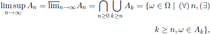
is called the upper limit of the sequence (A_n).

– The set of ω ∈ Ω belonging to all A_n except possibly to a finite number of them, that is,

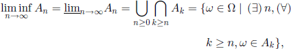
is called the lower limit of the sequence (A_n).

THEOREM 1.1.– (Borel-Cantelli lemma) Let (A_n) be a sequence of events in .

1. , them

2. and (A_n) is a sequence of independent events, then

Let (X_n) be a sequence of r.v. and X an r.v., all of them defined on the same probability space . The convergence of the sequence (X_n) to X will be defined as follows:

1. Almost sure

2. In probability if for any ε > 0,

.

3. In distribution (or weekly, or in law) pointwise in every continuity point of F_X, where F_Xn and F_X are the distribution functions of X_n and X, respectively.

4. In mean of order for all n ∈ N+, and if . The most commonly used are the cases p = 1 (convergence in mean) and p = 2 (mean square convergence).

The relations between these types of convergence are as follows:

[1.1]

The convergence in distribution of r.v. is a convergence property of their distributions (i.e. of their laws) and it is the most used in probability applications. This convergence can be expressed by means of characteristic functions.

THEOREM 1.2.– (Lévy continuity theorem) The sequence (X_n) converges in distribution to X if and only if the sequence of characteristic functions of (X_n) converges pointwise to the characteristic function of X.

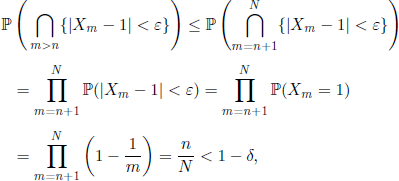
EXAMPLE 1.3.– Let X₁, X₂,… be independent r. v. such that and . We have , but X_n is not almost surely convergent to 1 as n → ∞.

Indeed, for any ∈ > 0 we have

Consequently, .

To analyze the convergence a.s., we recall the following condition: , if and only if, for any ∈ > 0 and 0 < δ < 1, there exists an n₀ such that for any n > n₀

[1.2]

As for any ∈ > 0, δ ∈ (0,1), and we have

it does not exist an n₀ such that relation [1.2] is satisfied, so we conclude that X_n does not converge a.s.

EXAMPLE 1.4.– Let us consider the probability space , with Ω = [0,1], , and the Lebesgue measure on . Let the r.v. X and the sequence of r.v be defined by

and

On the one hand, as

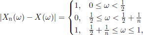
we obtain that . Thus (X_n) does not converge in probability. On the other hand, the characteristic functions of the r.v. , and X are

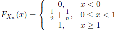
and, respectively,

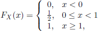
so .

Let us consider a sequence of r.v. (X_n,n ≥ 1) and suppose that the expected values , exist. Let

[1.3]

DEFINITION 1.5.– The sequence (X_n,n ≥ 1) is said to satisfy the weak or the strong law of large numbers if , respectively.

Obviously, if a sequence of r.v. satisfies the strong law of large numbers, then it also satisfies the weak law of large numbers.

The traditional name “law of large numbers” that is still in use nowadays should be clearly understood: it is indeed a “true” mathematical theorem! We do indeed still speak of laws of large numbers to express vaguely but correctly the sense of a convergence of frequency toward probability, but we also tend to believe sometimes that a return to equilibrium will always occur in the end, and this is a big error of which we are often unaware.

Let us present now some “classic laws of large numbers.”

THEOREM 1.6.– (Markov) Let (X_n,n ≥ 1) be a sequence of r.v. such that and If

[1.4]

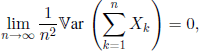
then (X_n, n ≥ 1) satisfies the weak law of large numbers.

PROOF.– Chebyshev’s inequality applied to Y_n defined in equation [1.3] yields

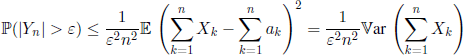
and thus we obtain

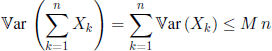
COROLLARY 1.7.– (Chebyshev) Let (X_n,n ≥ 1) be a sequence of independent r.v. such that If there exists an M, 0 < M < ∞, such that then (X_n,n ≥ 1) satisfies the weak law of large numbers.

PROOF.– In our case we have

and condition [1.4] is verified.

THEOREM 1.8.– (Kolmogorov) Let (X_n, n ≥ 1) be a sequence of independent r.v. such that , and 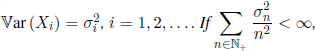, then (X_n,n ≥ 1) satisfies the strong law of large numbers.

COROLLARY 1.9.– In the settings of Corollary 1.7, the sequence of r.v. (X_n,n ≥ 1) satisfies the strong law of large numbers.

EXAMPLE 1.10.– Let (X_n) be a sequence of i.i.d. r.v. of distribution P.¹ For any Borel set B, the r.v. ll (X_n ∈ B) are i.i.d., with common expected value P(B). Using the law of large numbers, Corollary 1.9, we have

This argument justifies the estimation of probabilities by frequencies.

EXAMPLE 1.11.– Let (X_n) be a sequence of r.v. that take the values , , with probabilities and

We have and ar (X_k) = 2, k = 2,3,.... Consequently, the sequence (X_n) satisfies the strong law of large numbers (see Corollary 1.9).

EXAMPLE 1.12.– Let (X_n) be a sequence of r.v. that take the values , , with probabilities and

We have and , which yields

and

Consequently, the hypotheses of Theorem 1.6 are fulfilled and the sequence (X_n) satisfies the weak law of large numbers.

It is easy to see that in applications we often have to deal with random variables composed of an important number of independent elements. Under very general conditions, such sum variables are normally distributed. This fundamental fact can be mathematically expressed in one of the forms (depending on the conditions) of the central limit theorem. To state the central limit theorem, we consider (X_n, n ≥ 1) a sequence of r.v. and we introduce the following notation:

A central limit theorem gives sufficient conditions for the random variable

to converge in distribution to the standard normal distribution N(0, 1).

We see that, if the r.v. (X_n, n ≥ 1) are independent, then and are standard r.v., because and .

We give now a central limit theorem important in probability and mathematical statistics.

THEOREM 1.13.– Let (X_n, n ≥ 1) be a sequence of independent identically distributed r.v. with mean a and finite positive variance a². Then, the sequence of r.v. , is convergent in distribution to the normal distribution N(0,1). Z_n is said to be asymptotically normal.

PROOF.- Let φ(t) be the characteristic function of (X₁ — a) (hence of all (X_n — a), n ≥ 1). Then the characteristic function of Z_n is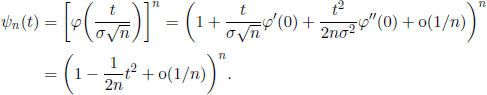

THEREFORE, and, using Theorem 1.2, we obtain .

COROLLARY 1.14.– (De Moivre-Laplace) If X ~ Bi(n,p) and q = 1 — p, then is asymptotically normal N(0,1), as n —>∞.

PROOF.- This result is a direct consequence of Theorem 1.13, because X = , with (X_n, n ≥ 1) i.i.d. random variables, X_n ~ Be(p).

EXAMPLE 1.15.– We roll a die n times and we consider the r.v. N = number of six. Starting from which value n of N do we have 9 out of 10 chances to get

As N is a binomial r.v. Bi(n, 1/6), for n large enough we can use Corollary 1.14 to approach the r.v. by a normal r.v. N(0, 1). Then, the condition can be written as . From relation which can be written as 2Φ(x) − 1 = 0.9,² we obtain x = 1.645 (using the table of the standard normal distribution). Thus we have nine out of 10 chances to have if the inequality 1.645 is satisfied, that is, if

EXAMPLE 1.16.– Suppose that the lifetime of a component is an exponentially distributed r.v. with parameter λ = 0.2 x 10^-3h^-1. When a component breaks down, it is immediately replaced with a new identical one. What is the probability that after 50,000 hours the component which will be working will be at least the 10th used from the beginning?

Let us denote by S_n the sum of n independent exponential random variables that represent the lifetimes of the first n components. From the properties of the exponential distribution, we have . Using Theorem 1.13, we can approach by a standard normal random variable, which is equivalent to saying that we can approach S_n by a normal r.v. N(n/λ, /λ) = N(5000n, 5000). The fact that the component which will be working after 50,000 hours will be at least the 10th used means that we have S₉< 50,000, so we need only to compute , with S₉ ~ N (45,000,15,000). Thus we obtain the required probability

EXAMPLE 1.17.– A restaurant can serve 75 meals a day. We know from experience that 20% of the clients that reserved would not eventually show up.

a) The owner of the restaurant accepts 90 reservations. What is the probability that more than 50 clients show up?

b)How many reservations should the owner of the restaurant accept in order to have a probability greater than or equal to 0.9 that he will be able to serve all the clients who will show up?

If n is the number of clients who reserved, the number N of clients who will come has a binomial distribution with parameters n and p = 0.8. Using corollary 1.14, this binomial distribution is approached by a normal distribution with the same mean and variance.

a) Consequently,

b) We have to solve the inequality with respect to N. On the one hand, we have

and, on the other hand, we have $(1.281) = 0.9. So we need to have , that is, . By letting we get the inequality 0.8x² + 0.5124x − 75 < 0 and finally obtain x < 9.367503, 097, i.e. n ≤ 87.

1.2. The notion of stochastic process

A stochastic or a random process is a family of r.v. defined on the same probability space , with values in a measurable space .

The set E can be either or , and in this case is the σ-algebra of Borel sets, or an arbitrary finite or countable infinite discrete set, and in this case .

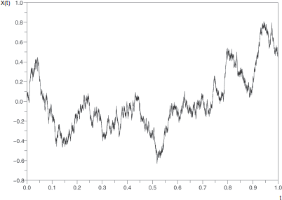
The index set I is usually (in this case the process is called chain) or , and the parameter t is interpreted as being the time. The function is called a realization or a sample path of the process (see Figure 1.1).

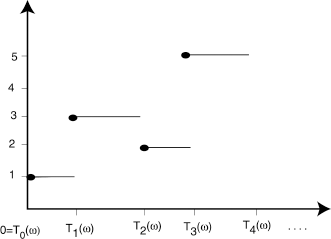
If the evolution of a stochastic process is done by jumps from state to state and if almost all its sample paths are constant except at isolated jump times, then the process is called a jump process.

EXAMPLE 1.18.– Let us consider the process , with state space E = , describing the evolution of a population, the number of failures of a component, etc. Then X_t(ω) = X(t, ω) = i ∈ E means that the population has i individuals at time t, or that the component has failed i times during the time interval (0, t].

The times T₀(ω),T₁(ω), ... (Figure 1.2) are the jump times (transition times) for the particular sample path ω ∈ Ω. The r.v. ζ = sup_n T_n is the lifetime of the process.

The stochastic processes can be studied either by means of their finite-dimensional distributions or by considering the type of dependence between the r.v. of the process. In the latter case, the nature of the process is given by this type of dependence.

The distribution of a stochastic process X, i.e. , is specified by the knowledge of its finite-dimensional distributions. For a real-valued

process we define

[1.5]

for any t₁, ..., t_n ∈ I and x₁, ..., x_n ∈ .

The process is said to be given if all the finite-dimensional distributions F_{t1 ,...,tn} (·, ..., ·), t₁, ..., t_n ∈ I, are given.

The finite-dimensional distributions must satisfy the following properties:

1) for any permutation (i₁, ..., i_n) of (1, ..., n),

2) for any 1 ≤ k ≤ n and x₁, ..., x_n ∈ ,

.

Let X = (X_t;t ∈ I) and Y = (Y_t;t ∈ I) be two stochastic processes on the same probability space , with values in the same measurable space (E, ∈ ).

DEFINITION 1.19.– (Stochastically equivalent processes in the wide sense) If two stochastic processes X and Y satisfy

for all n ∈ N^∗, t₁, ..., t_n ∈ I, and A₁, ..., A_n ∈ E, then they are called stochastically equivalent in the wide sense.

DEFINITION 1.20.– (Stochastically equivalent processes) If two stochastic processes X and Y satisfy

then they are called stochastically equivalent.

DEFINITION 1.21.– (Indistinguishable processes) If two stochastic processes X and Y satisfy

then they are called indistinguishable.

PROPOSITION 1.22.– We have the following implications: X,Y indistinguishable X,Y stochastically equivalent X, Y stochastically equivalent in the wide sense.

PROPOSITION 1.23.– If the processes X and Y are stochastically equivalent and right continuous, then they are indistinguishable.

DEFINITION 1.24.– (Version or modification of a process) If the process Y is stochastically equivalent to the process X, then we say that Y is a version or a modification of the process X.

DEFINITION 1.25.– (Continuous process) Aprocess X with values in aBorel space (E, ∈ ) is said to be continuous a.s. if, for almost all ω, the function is continuous.

PROPOSITION 1.26.– (Kolmogorov continuity criterion) A real process X has a continuous modification if there exist the constants α, β, C > 0, such that for all t and s.

1.3. Martingales

1.3.1. Stopping time

Let be a probability space. An increasing sequence of σ-algebras, , is called a filtration of . A sequence (X_n,n ∈ ) of r.v. is said to be F-adapted if X_n is _n -measurable for all . Usually, a filtration is associated with the sequence of r.v. , that is, we have _n and the sequence will be F-adapted. This is called the natural filtration of .

DEFINITION 1.27.– Let be a filtration of . A stopping time for F (or F-adapted, or F-stopping time) is an r.v. T with values in satisfying one of the following (equivalent) conditions:

If , T is said to be adapted to the sequence . In this case we note .

EXAMPLE 1.28.– (Hitting time) Let be a sequence of r.v. with values in ^d and . The r.v. T = inf is a stopping time, adapted to the sequence (X_n, n ∈ ) and is called the hitting time of B. Indeed,

Properties of stopping times

1.The set is a σ-algebra called the σ-algebra of events prior to T.

2. If S and T are stopping times, then S + T, S ⋀ T, and S ⋁ T are also stopping times.

3.If is a sequence of stopping times, then is also a stopping time.

4.If S and T are stopping times such that S ≤ T, then _s ⊆ _T.

PROPOSITION 1.29.– (Wald identity) If T is a stopping time with finite expected value, adapted to an i.i.d. and integrable random sequence (X_n,n ∈ ), then

1.3.2. Discrete-time martingales

We will consider in the following that every filtration F is associated with the corresponding random sequence.

DEFINITION 1.30.– A sequence of r.v. (X_n, n ∈ ) is an

1)X_n F-martingale if

2)F-submartingale if it satisfies (a), (b), and (c) with <.

3) F-supermartingale if it satisfies (a), (b), and (c) with >.

Note that condition (c) is equivalent to .

EXAMPLE 1.31.– Let be a sequence of i.i.d. r.v. such that and . The random walk (see section 2.2) , is a submartingale for the natural filtration of (ζ_n) if p > 1/2, a martingale if p = 1/2, and a supermartingale if p < 1/2. Indeed, we have Consequently,

EXAMPLE 1.32.– Let X be a real r.v. with and let F be an arbitrary filtration. Then, the sequence is a martingale. Indeed,

EXAMPLE 1.33.– (A martingale at the casino) A gambler bets 1 euro the first time, if he loses he bets 2 the second time, etc. ^k−1 the kth time. He stops gambling when he wins for the first time. At every play, he wins or loses his bet with a probability of 1/2. This strategy will make him eventually win the game. Indeed, when he stops playing at a random time N, he would have won 2^N − (1 + 2 + ··· + 2^{N − 1}) = 1.

If X_n is the r.v. defined as the fortune of the gambler after the nth game, we have

if he loses up to the nth game. Consequently (X_n+1 | X_n,..., X₁) = X_n.

On the other hand, the expected value of the loss is

because N is a geometrically distributed r.v. with parameter 1/2 and for n ≥ N. Consequently, the strategy of the player is valid only if his initial fortune is greater than the casino’s.

1.3.3. Martingale convergence

THEOREM 1.34.– (Doob’s convergence theorem) Every supermartingale, submartingale or martingale bounded in L¹ converges a.s. to an integrable r.v.

EXAMPLE 1.35.– If X is an r.v. on with finite expected value and is a filtration of , then

THEOREM 1.36.– If (X_n) is an uniformly integrable martingale, i.e.

then there exists X integrable such that , and we have.

A martingale (X_n) for is said to be a square integrable if for all n ≥ 1.

THEOREM 1.37.– (Strong convergence theorem) If (X_n) is a square integrable martingale, then there exists an r.v. X such that .

THEOREM 1.38.– (Stopping theorem) Let (X_n) be a martingale (resp. a submartingale) for (_n). If S and T are two stopping times adapted to (_n) such that

1) and

2) and

then

1.3.4. Square integrable martingales

Let (M_n, n ≥ 0) be a square integrable martingale, i.e.

The process is a submartingale and Doob’s decomposition gives

where X_n is a martingale, and < M >_n is a predictable increasing process, that is, -measurable for all n ≥ 1.

THEOREM 1.39.– If (M_n) is a square integrable martingale, with predictable process < M >_n, and if

1)

2)

for all

then

and

where (a_n) is a sequence increasing to infinity.

1.4. Markov chains

Markov chains and processes represent probabilistic models of great importance for the analysis and study of complex systems. The fundamental concepts of Markov modeling are the state and the transition.

1.4.1. Markov property

It is clear that the situation of a physical system at a certain moment can be completely specified by giving the values of a certain number of variables that describe the system. For instance, a physical system can often be specified by giving the values of its temperature, pressure, and volume; in a similar way, a particle can be specified by its coordinates with respect to a coordinate system, by its mass and speed. The set of such variables is called the state of the system, and the knowledge of the values of these variables at a fixed moment allows us to specify the state of the system, and, consequently, to describe the system at that precise moment.

Usually, a system evolves in time from one state to another, and is thus characterized by its own dynamics. For instance, the state of a chemical system can change due to a modification in the environment temperature and/or pressure, whereas the state of a particle can change because of interaction with other particles. These state modifications are called transitions.

In many applications, the states are described by continuous variables and the transitions may occur at any instant. To simplify, we will consider a system with a finite number of states, denoted by E = {1, 2, . . ., N}, and with transitions that can occur at discrete-time moments. So, if we set X(n) for the state of the system at time n, then the sequence X(0), X(1), . . ., X(n) describes the “itinerary” of the system in the state space, from the beginning of the observation, up to the fixed time n; this sequence is called a sample path (realization or trajectory) of the process (see section 1.2).

In most of the concrete situations, the observation of the process makes us come to the conclusion that the process is random. Consequently, to a sample path of the process a certain probability

needs to be associated. Elementary techniques of probability theory show that these probabilities can be expressed in terms of the conditional probabilities

for all and for any states i₀, i₁, . . ., i_n+1 ∈ E. This means that it is necessary to know the probability that the system is in a certain state i_n+1 ∈ E after the (n + 1)th transition, , knowing its history up to time n. Computing all these conditional probabilities renders the study of a real phenomenon modeled in this way very complicated. The statement that the process is Markovian is equivalent to the simplifying hypothesis that only the last state (i.e. the current state) counts for its future evolution. In other words, for a Markov process we have (the Markov property)

[1.6]

DEFINITION 1.40.– The sequence of r.v. defined on , with values in the set E, is called a Markov chain (or discrete-time Markov process) with a finite or countable state space, if the Markov property is satisfied.

A Markov chain is called nonhomogenous or homogenous (with respect to time) whether or not the common value of the two members of [1.6] (i.e. the function p(n, i, j)) depends on n. This probability is called transition function (or probability) of the chain.

For more details on the study of discrete-time Markov processes with finite or countable state space, see [CHU 67, IOS 80, KEM 60, RES 92].

So, the Markovian modeling is adapted to physical phenomena or systems whose behavior is characterized by a certain memoryless property, in the sense specified in [1.6]. For real applications, it is very difficult often even impossible to know whether a physical system has a Markovian behavior or not; in fact, it is important to be able to justify this Markovian behavior (at least as a first approximation of the phenomenon) and thus to obtain a model useful for the study of the phenomenon.

Note that the Markovian modeling can also be used in the case in which a fixed number of states, not only the last one, determines the future evolution of the phenomenon. For instance, suppose that we take into account the last two visited states. Then, we can define a new process with n² states, where the states are defined as couples of states of the initial process; this new process satisfies property [1.6] and the Markovian model is good enough, but with the obvious drawback of computational complexity.

PROPOSITION 1.41.– If the Markov property (1.6) is satisfied, then

[1.7]

for all and i₀, i₁, ..., i_n,j₁, ...j_m ∈ E.

REMARK 1.42.– The more general relation

[1.8]

can be proved for any A ∈ σ(X_k;k ≥ n + 1). The equalities between conditional probabilities have to be understood in the sense of almost surely . We will often write instead of

1.4.2. Transition function

Throughout this chapter, we will be concerned only with homogenous Markov chains and the transition function will be denoted by p(i, j). It satisfies the following properties:

[1.9]

[1.10]

A matrix that satisfies [1.9] and [1.10] is said to be stochastic.

From [1.8], taking A = (X_n+1 = j), we obtain

[1.11]

The probability does not depend on n and will be denoted by p^(m)(i, j).

The matrix p = (p(i, j); i, j ∈ E) is called the transition matrix of the chain, and p^(m)(i, j) is the (i, j) element of the matrix p^m.

From the following matrix equality

[1.12]

we obtain

[1.13]

for all . Equality [1.12] (or [1.13]) is called the Chapman-Kolmogorov identity (or equality).

EXAMPLE 1.43.– Binary component. Consider a binary component starting to work at time n = 0. The lifetime of the component has a geometric distribution on of parameter p. When a failure occurs, it is replaced with a new, identical component. The replacement time is a geometric random variable of parameter q. Denote by 0 the working state, by 1 the failure state, and let X_n be the state of the component at time n ≥ 0. Then X_n is an r.v. with values in E = {0, 1}. It can be shown that is a Markov chain with state space E and transition matrix

Using the eigenvalues of the matrix p, we obtain

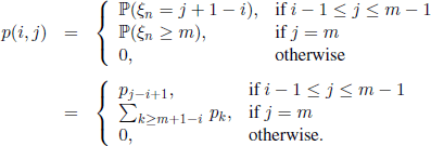
EXAMPLE 1.44.– A queuing model. A service unit (health center, civil service, tasks arriving in a computer, etc.) can serve customers (if any) at times 0,1, 2,.... We suppose that during the time interval (n, n + 1] there are ξ_n clients arriving, , where the r.v. ξ₀, ξ₁, ξ₂, ... are i.i.d. and p_k, k ≥ 0, Σ_k≥0pk = 1. Let m be the number ofplaces available in the queue (m can also take the value +∞). When a customer arrives and sees m clients waiting to be served, then he leaves without waiting. Let X_n be the number of customers in the queue at time n (including also the one that is served at that moment). We have

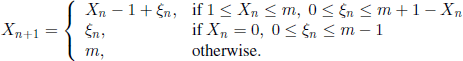
The process is a Markov chain with state space E = {0,1,…, m}, because X_n+1 depends only on the independent r.v. X_n and ξ_n. The transition function is given by

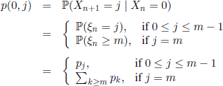
and, for 1≤i≤m

EXAMPLE 1.45.– Storage model. A certain product is stocked in order to face a random demand. The stockpile can be replenished at times 0, 1, 2, … and the demand in the time interval (n, n + 1] is considered to be a discrete -valued r.v. ξ_n. The r.v. ξ₀, ξ₁, ξ₂, ... are supposed to be i.i.d. and

The stocking strategy is the following: let m, M ∈ , be such that m < M; if, at an arbitrary time , the inventory level is less or equal to m, then the inventory is brought up to M. Whereas, if the inventory level is greater than m, no replenishment is undertaken.

If X_n denotes the stock level just before the possible supply at time n, we have

The same approach as in example 1.44 can be used in order to show that is a Markov chain and subsequently obtain its transition function.

1.4.3. Strong Markov property

Let be a Markov chain defined on , with values in E. Consider the filtration be a stopping time for the chain X (i.e. for the filtration and be the σ-algebra of events prior to τ. We want to obtain the Markov property (relation [1.6]) in case that the “present moment” is random.

PROPOSITION 1.46.– For all such that , we have

[1.14]

REMARK 1.47.– We can prove more general relations as follows: if B is an event subsequent to τ, i.e. B ∈ σ(X_τ+k, k ≥ 0), then

[1.15]

[1.16]

DEFINITION 1.48.– Relation [1.15] is called the strong Markov property.

If X₀ = j a.s., j ∈ E, then the r.v.

with the convention inf Ø = ∞, is called the sojourn time in state j and it is a stopping time for the family .

PROPOSITION 1.49.– The sojourn time in a state j ∈ E is a geometric r.v. of parameter 1 − p(j, j) with respect to the probability for .

1.5. State classification

DEFINITION 1.50.– Let X = (X_n, n ∈ ) be a Markov chain defined on , with values in E (finite or countable). We call a state j ∈ E accessible from state i ∈ E (we write i → j) if there exists an such that p⁽ⁿ⁾(i, j) > 0. The states i and j are said to communicate if i → j and j → i; this will be denoted by i ↔ j.

Note that relation i → j is transitive, i.e. if i → j and j → k then i → k.

DEFINITION 1.51.– A class of states is a subset C of E that satisfies one of the two following properties:

1)The set C contains only one state i ∈ E and relation i ↔ i is not verified.

2)For all i, j ∈ C we have i ↔ j and C is maximal with this property, i.e. it is not possible to increase C by another state which communicates with all the other states of C.

EXAMPLE 1.52.– Let X = (X_n, n ∈ ) be a Markov chain with values in E = {0, 1, 2, 3} and of transition matrix

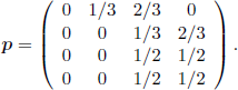
The matrices p^m, m ≥ 2, have all the entries on the second column equal to zero. Consequently, the classes are C₁= {0}, C₂ = {1}, and C₃ = {2,3}.

DEFINITION 1.53.– 1. A property concerning the states of E, such that the validity for a state i ∈ E implies the validity for all states from the class of i, is called a class property.

2. A class of states C is called closed if Σ_j∈C p(i, j) = 1 for all i ∈ C. In other words, the matrix (p(i,j); i, j ∈ C) is a stochastic matrix; thus, Σ_j∈c p⁽ⁿ⁾ {i, j) = 1 for all i ∈ C and n ∈ .

3. If a closed class contains only one state, then this state is called absorbing

4. If the state space E consists of only one closed class, then the chain is called irreducible.

5.A state i ∈ E is said to be essential if i → j yields j → i; otherwise i is called inessential.

6. If i → i, then the greatest common divisor of n ∈ such that p⁽ⁿ⁾(i, i) > 0 is called the period of i and will be denoted by d%. If d_i = 1, then the state i is called aperiodic.

PROPOSITION 1.54.– Let C be a closed class of period d and C₀, C₁, …, C_d−1 be the cyclic subclasses.

1. If i ∈ C_r and p⁽ⁿ⁾(i,j) > 0, then j ∈ C_n+r.

2.If i ∈ C_r, we have

(The class subscripts are considered mod d).

We will denote by , the probabilities on σ(X_n; n ∈ ) defined by

and by _i the corresponding expected values.

If α = (α(i), i ∈ E) is a probability on E, i.e. then and is the corresponding expected value.

DEFINITION 1.55.– Let η_i,i ∈ E, be the first-passage time to state i. The state i ∈ E is said to be recurrent (or persistent) if . In the opposite case, i.e. if , the state i is said to be transient. If i is a recurrent state, then if , i is said to be positive recurrent, and if μ_i = ∞, then i is said null recurrent.

PROPOSITION 1.56.– A state i ∈ E is recurrent or transient, if the series is divergent, respectively convergent.

PROPOSITION 1.57.– Let (X_n, n ∈ ) be a Markov chain with finite state space E. Then:

1) there exists at least a recurrent state;

2) a class is recurrent iff it is closed.

PROPOSITION 1.58.– Let X = (X_n, n ∈ ) be a Markov chain with finite state space. Then any recurrent class C of X is positive. If the chain X is irreducible, then it is positive recurrent (i.e. all states are positive recurrent).

1.5.1. Stationary probability

DEFINITION 1.59.– A probability distribution π on E is said to be stationary or invariant for the Markov chain X = (X_n, n ∈ ) with transition matrix P = (p(i, j); i, j ∈ E) if, for all j ∈ E,

[1.17]

Relation [1.17] can be written in matrix form

[1.18]

where π = (π(i); i ∈ E) is a row vector. From [1.18] we can easily prove that

[1.19]

and

[1.20]

PROPOSITION 1.60.– We suppose that the transition matrix is such that the limits

[1.21]

exist for all i, j ∈ E and do not depend on i. Then, there are two possibilities:

1) π(j) = 0 for all j ∈ E and, in this case, there is no stationary probability;

2) Σ_j∈E π(j) = 1 and, in this case, π = (π(j); j ∈ E) is a stationary probability and it is unique.

DEFINITION 1.61.– A Markov chain is said to be ergodic if, for all i, j ∈ E, the limits lim_n→∞p⁽ⁿ⁾(i, j) exist, are positive, and do not depend on i.

PROPOSITION 1.62.– An irreducible, aperiodic, and positive recurrent Markov chain is ergodic.

PROPOSITION 1.63.– A finite Markov chain is ergodic if and only if

[1.22]

A Markov chain verifying [1.22] is called regular.

PROPOSITION 1.64.– A Markov chain with finite or countable state space E has a unique stationary probability if and only if the state space contains one and only one recurrent positive class.

COROLLARY 1.65.– A finite ergodic Markov chain (i.e. regular) has a unique stationary probability.

1.6. Continuous-time Markov processes

The concept of Markovian dependence in continuous time was introduced by A. N. Kolmogorov in 1931. The first important contributions are those of B. Pospisil, W. Feller, and W. Doeblin, and the standard references are [BLU 68, DYN 65, GIH 74].

1.6.1. Transition function

Let E be a finite or countable set and , be a matrix function with the properties:

[1.23]

where δ_ij is the Kronecker symbol.

A family of r.v. with values in E is called a Markov process homogenous with respect to time, with state space E, if

[1.24]

for all 0 ≤ t₀ < t₁ <…< t_n, t ≥ 0, i₀, i₁, …,i_n−1, i, j ∈ E, n ≤ 1. We will suppose that the sample paths t → X(t, ω) are right-continuous with left limits a.s. The matrix P(t), called the transition matrix function of the process, satisfies the Chapman-Kolmogorov equation

[1.25]

which can be written under matrix form

The functions p_ij (t) have some remarkable properties:

1) For all i, j ∈ E, the function P_ij(t) is uniformly continuous on [0, ∞).

2) For all i,j ∈ E, the function p_ij (t) is either identically zero, or positive, on (0, ∞).

3) For all exists and it is finite.

4) For all exists and . A state z is said to be stable if q_i < ∞, instantaneous if q_i = ∞, and absorbing if q_i = 0.

PROPOSITION 1.66.– If E is finite, then there is no instantaneous state.

PROPOSITION 1.67.– The sample paths of the process are right continuous a.s. if and only if there is no instantaneous state.

1.6.2. Kolmogorov equations

If q_i < ∞ for all i ∈ E, then the matrix Q = (qij,i,j ∈ E), where q_ii = —q_i, is called the infinitesimal generator of the process or transition intensity matrix. Generally, we have q_ij ≥ 0 for i ≠ j and q_ii ≤ 0. Additionally,

[1.26]

If E is finite, then [1.26] becomes

[1.27]

Relation [1.27] is a necessary and sufficient condition such that p_ij (t) satisfy the differential equations

[1.28]

or, in matrix form,

Equations [1.28] are called Kolmogorov backward equations. In addition, if q_j < ∞, j ∈ E, and the limit

is uniform with respect to i ≠ j, then we have

[1.29]

Equations [1.29] are called Kolmogorov forward equations.

Note the important fact that, if E is finite, then the two equations [1.28] and [1.29] are satisfied. In this case, from these two systems of equations, with initial conditions p_ij(0)= δ_ij, i, j ∈ E (or under matrix form P(0) = I), we obtain

[1.30]

Consequently, the transition intensity matrix Q uniquely determines the transition matrix function P(t).

The first jump time or the sojourn time in a state is defined by

Then is the distribution function of the sojourn time in state i.

PROPOSITION 1.68.– For i, j ∈ E, we have

[1.31]

and the r.v. T₁ and X_T1 are -independent.

The successive jump times of the process can be defined as follows:

The lifetime of the process is the r.v. , then the process is regular (non-explosive); in the opposite case, if , the process is called non-regular (explosive).

If T_n+1 > T_n a.s. for all n ≥ 1, then (X(t),t ≥ 0) is said to be a jump process.

PROPOSITION 1.69.– There exists a stochastic matrix (a_ij,i, j ∈ E) with a_ii = 0, i ∈ E, such that

[1.32]

This means that the successively visited states form a Markov chain Y_n = X_Tn, called the embedded chain, with transition function A. Given the successively visited states of the process, the sojourn times in different states are mutually independent.

REMARK 1.70.– We have

[1.33]

PROPOSITION 1.71.– (Reuter’s explosion condition) A jump Markov process is regular iff the only non-negative bounded solution of equation Qy = y is y = o.

PROPOSITION 1.72.– A necessary and sufficient condition for a Markov process (X(t),t ≥ 0) to be regular is a.s.

PROPOSITION 1.73.– (Kolmogorov integral equation) For i, j ∈ E, we have

[1.34]

for i non-absorbing, and P_ij (t) = δ_ij for i absorbing.

Let us denote by η_i the first-passage time to state i, i.e. η_i = inf (t ≥ T₁|X_t=i). A state i ∈ E is said to be:

– recurrent if ;

– transient if ;

– positive recurrent if it is recurrent and ;

– null recurrent if it is recurrent and μ_ii = ∞.

For α = (α_i, i ∈ E) a probability on E, we define

The probabilities Pi(t) = P_α(X_t = i), i ∈ E, t ≥ 0, are called state probabilities. If p_i = p_i(0) = P_α(X₀ = j), j ∈ E, then the state probabilities satisfy the equations

[1.35]

A probability π = (π_j, j ∈ E) on E is said to be stationary or invariant if P_π(X_t = j) = π_j, for all j ∈ E, t ≥ 0. This condition can be written in the matrix form πP(t) = π for all t ≥ 0. From [1.35] it can be inferred that (π_j, j ∈ E) is stationary if and only if .

A Markov process (X(t),t > 0) is said to be ergodic if there exists a probability π on E such that, for all i, j ∈ E, we have

or, equivalently,

for all i ∈ E.

PROPOSITION 1.74.– For any state i of E, we have

PROPOSITION 1.75.– If the Markov process (X(t),t > 0) is irreducible (i.e. the chain (Y_n, n ∈ ) is so) and it has an invariant probability π, then for any positive and bounded function g on E, we have

1.7. Semi-Markov processes

A semi-Markov process is a natural generalization of a Markov process. Its future evolution depends only on the time elapsed from the last transition.

The semi-Markov processes that we will present are minimal semi-Markov processes associated with Markov renewal processes, with finite state spaces E. Consequently, we do not have to take into account instantaneous states and the sojourn times of a process form, almost surely on ₊, a dense set.

1.7.1. Markov renewal processes

Let the functions Q_ij, i, j ∈ E, defined on the real line, be non-decreasing, right continuous, and such that Q_ij (∞) ≤ 1; they will be called mass functions. Besides, if we have

with , the matrix function Q(t) = (Qij(t),i, j ∈ E), t ∈ ₊, is called a semi-Markov kernel (matrix) on the state space E. On E we consider the σ-algebra .

Let us consider the Markov transition function P((i, s), {j} x[0,t]) defined on the measurable space by

Then [BLU 68, DYN 65, GIH74], there exists a Markov chain ((J_n,T_n),n ∈ ) with values in , such that the transition function is given by

[1.36]

If we set X₀ = T₀, X_n =T_n — T_n_₁, n ≥ 1, then the process ((J_n, X_n),n ∈ ) is a Markov chain with values in E x R₊ and a transition function given by

[1.37]

Obviously,

where

DEFINITION 1.76.– The processes ((J_n,T_n), n ∈ ) and ((Jn,Xn),n ∈ ) are called Markov renewal process (MRP) and, respectively, J — X process.

Note that (J_n,n ∈ ) is a Markov chain with values in E and transition matrix p = (P_ij, i, j ∈ E), with p_ij = Q_ij(∞).

The n-fold matrix Stieltjes convolution is defined by

and we have

[1.38]

1.7.2. Semi-Markov processes

We will suppose that

and define

DEFINITION 1.77.– The jump stochastic process (Z_t, t ∈ ₊), where

[1.39]

is said to be a semi-Markov process associated with the MRP (J_n, T_n).

We only present some notions regarding semi-Markov processes here, for they will be detailed in Chapter 5.

The jump times are T₀ < T₁ < T₂ < · · · < T_n < … and the inter-jump times are X₁, X₂, ….

Obviously,

For any i, j ∈ E we define the distribution function F_ij by

Note that F_ij is the distribution function of the sojourn time in state i, knowing that the next visited state is j. These distribution functions are called conditional transition functions.

The transition functions of the semi-Markov process are defined by

[1.40]

We denote by N_j(t) the number of times the semi-Markov process visits state j during the time interval (0, t]. For i, j ∈ E we let

The function t → Ψ_ij(t) is called the Markov renewal function. This function is the solution of the Markov renewal equation

[1.41]

The transition probabilities [1.40] satisfy the Markov renewal equation

[1.42]

---

1. In fact, the distribution (or law) of an r.v. is a probability on , i.e. on the Borel sets of .

2. Φ is the d.f. of N (0, 1).