
Chapter 8
Polynomials, Curve Fitting, and Interpolation
Polynomials are mathematical expressions that are frequently used for problem solving and modeling in science and engineering. In many cases an equation that is written in the process of solving a problem is a polynomial, and the solution of the problem is the zero of the polynomial. MATLAB has a wide selection of functions that are specifically designed for handling polynomials. How to use polynomials in MATLAB is described in Section 8.1.
Curve fitting is a process of finding a function that can be used to model data. The function does not necessarily pass through any of the points, but models the data with the smallest possible error. There are no limitations to the type of the equations that can be used for curve fitting. Often, however, polynomial, exponential, and power functions are used. In MATLAB curve fitting can be done by writing a program or by interactively analyzing data that is displayed in the Figure Window. Section 8.2 describes how to use MATLAB programming for curve fitting with polynomials and other functions. Section 8.4 describes the basic fitting interface that is used for interactive curve fitting and interpolation.
Interpolation is the process of estimating values between data points. The simplest kind of interpolation is done by drawing a straight line between the points. In a more sophisticated interpolation, data from additional points is used. How to interpolate with MATLAB is discussed in Sections 8.3 and 8.4.
8.1 POLYNOMIALS
Polynomials are functions that have the form:
![]()
The coefficients an, an − 1, …, a1, a0 are real numbers, and n which is a nonnegative integer, is the degree, or order, of the polynomial.
Examples of polynomials are:
| f(x) = 5x2 + 6x2 + 7x + 3 | polynomial of degree 5. |
| f(x) = 2x2 −4x + 10 | polynomial of degree 2. |
| f(x) = 11x − 5 | polynomial of degree 1. |
A constant (e.g., f(x) = 6) is a polynomial of degree 0.
In MATLAB, polynomials are represented by a row vector in which the elements are the coefficients an, an − 1, …, a1, a0. The first element is the coefficient of the x with the highest power. The vector has to include all the coefficients, including the ones that are equal to 0. For example:
| Polynomial | MATLAB representation |
| 8x + 5 | p = [8 5] |
| 2x2 − 4x + 10 | d = [2 −4 10] |
| 6x2 − 150, MATLAB form: 6x2 + 0x − 150 | h = [6 0 −150] |
| 5x5 + 6x2 − 7x, MATLAB form: 5x5 + 0x4 + 0x3 + 6x2 − 7x + 0 | c = [5 0 0 6 −7 0] |
8.1.1 Value of a Polynomial
The value of a polynomial at a point x can be calculated with the function polyval that has the form:

x can also be a vector or a matrix. In such a case the polynomial is calculated for each element (element-by-element), and the answer is a vector, or a matrix, with the corresponding values of the polynomial.
Sample Problem 8-1: Calculating polynomials with MATLAB
For the polynomial f(x) = x5 − 12.1x4 + 40.59x3 − 17.015x2 − 71.95x + 35.88 :
(a) Calculate f(9).
(b) Plot the polynomial for −1.5 ≤ x ≤ 6.7.
Solution
The problem is solved in the Command Window.
(a) The coefficients of the polynomials are assigned to vector p. The function polyval is then used to calculate the value at x = 9.
>> p = [1 -12.1 40.59 -17.015 -71.95 35.88];

>> polyval(p,9)

ans =

  7.2611e+003
(b) To plot the polynomial, a vector x is first defined with elements ranging from −1.5 to 6.7. Then a vector y is created with the values of the polynomial for every element of x. Finally, a plot of y vs. x is made.

The plot created by MATLAB is presented below (axis labels were added with the Plot Editor).

8.1.2 Roots of a Polynomial
The roots of a polynomial are the values of the argument for which the value of the polynomial is equal to zero. For example, the roots of the polynomial f(x) = x2 − 2x − 3 are the values of x for which x2 − 2x − 3 = 0, which are x = −1 and x = 3.
MATLAB has a function, called roots, that determines the root, or roots, of a polynomial. The form of the function is:

For example, the roots of the polynomial in Sample Problem 8-1 can be determined by:

The roots command is very useful for finding the roots of a quadratic equation. For example, to find the roots of f(x) = 4x2 + 10x − 8, type:
>> roots([4 10 -8])

ans =

   -3.1375

    0.6375
When the roots of a polynomial are known, the poly command can be used for determining the coefficients of the polynomial. The form of the poly command is:

For example, the coefficients of the polynomial in Sample Problem 8-1 can be obtained from the roots of the polynomial (see above) by:
>> r=[6.5 4 2.3 -1.2 0.5];

>> p=poly(r)

p =

    1.0000  -12.1000  40.5900  -17.0150  -71.9500  35.8800
8.1.3 Addition, Multiplication, and Division of Polynomials
Addition:
Two polynomials can be added (or subtracted) by adding (subtracting) the vectors of the coefficients. If the polynomials are not of the same order (which means that the vectors of the coefficients are not of the same length), the shorter vector has to be modified to be of the same length as the longer vector by adding zeros (called padding) in front. For example, the polynomials
f1(x) = 3x6 + 15x5 − 10x3 − 3x2 + 15x − 40 and f2(x) = 3x3 − 2x − 6 can be added by:

Multiplication:
Two polynomials can be multiplied using the MATLAB built-in function conv, which has the form:

• The two polynomials do not have to be of the same order.
• Multiplication of three or more polynomials is done by using the conv function repeatedly.
For example, multiplication of the polynomials f1(x) and f2(x) above gives:
>> pm=conv(p1,p2)

pm =

     9  45  -6  -78  -99  65  -54  -12  -10  240
which means that the answer is:
9x9 + 45x8− 6x7 − 78x6 − 99x5 + 65x4 − 54x3 − 12x2 − 10x + 240
Division:
A polynomial can be divided by another polynomial with the MATLAB built-in function deconv, which has the form:

For example, dividing 2x3 + 9x2 + 7x − 6 by x + 3 is done by:


An example of division that gives a remainder is 2x6 − 13x5 + 75x3 + 2x2 − 60 divided by x2 − 5:

![]()
8.1.4 Derivatives of Polynomials
The built-in function polyder can be used to calculate the derivative of a single polynomial, a product of two polynomials, or a quotient of two polynomials, as shown in the following three commands.
k = polyder(p) |
Derivative of a single polynomial. p is a vector with the coefficients of the polynomial. k is a vector with the coefficients of the polynomial that is the derivative. |
k = polyder(a,b) |
Derivative of a product of two polynomials. a and b are vectors with the coefficients of the polynomials that are multiplied. k is a vector with the coefficients of the polynomial that is the derivative of the product. |
[n d] = polyder(u,v) |
Derivative of a quotient of two polynomials. u and v are vectors with the coefficients of the numerator and denominator polynomials. n and d are vectors with the coefficients of the numerator and denominator polynomials in the quotient that is the derivative. |
The only difference between the last two commands is the number of output arguments. With two output arguments MATLAB calculates the derivative of the quotient of two polynomials. With one output argument, the derivative is of the product.
For example, f1(x) = 3x2 − 2x + 4, and f2(x) = x2 + 5, the derivatives of 3x2 − 2x + 4, (3x2 − 2x + 4)(x2 + 5), and ![]() can be determined by:
can be determined by:

8.2 CURVE FITTING
Curve fitting, also called regression analysis, is a process of fitting a function to a set of data points. The function can then be used as a mathematical model of the data. Since there are many types of functions (linear, polynomial, power, exponential, etc.), curve fitting can be a complicated process. Many times one has some idea of the type of function that might fit the given data and will need only to determine the coefficients of the function. In other situations, where nothing is known about the data, it is possible to make different types of plots that provide information about possible forms of functions that might fit the data well. This section describes some of the basic techniques for curve fitting and the tools that MATLAB has for this purpose.
8.2.1 Curve Fitting with Polynomials; The polyfit Function
Polynomials can be used to fit data points in two ways. In one the polynomial passes through all the data points, and in the other the polynomial does not necessarily pass through any of the points but overall gives a good approximation of the data. The two options are described below.
Polynomials that pass through all the points:
When n points (xi, yi) are given, it is possible to write a polynomial of degree n − 1 that passes through all the points. For example, if two points are given it is possible to write a linear equation in the form of y = mx + b that passes through the points. With three points, the equation has the form of y = ax2 + bx + c. With n points the polynomial has the form an − 1 xn − 1 + an − 2 xn − 2 + … + a1x + a0. The coefficients of the polynomial are determined by substituting each point in the polynomial and then solving the n equations for the coefficients. As will be shown later in this section, polynomials of high degree might give a large error if they are used to estimate values between data points.
Polynomials that do not necessarily pass through any of the points:
When n points are given, it is possible to write a polynomial of degree less than n − 1 that does not necessarily pass through any of the points but that overall approximates the data. The most common method of finding the best fit to data points is the method of least squares. In this method, the coefficients of the polynomial are determined by minimizing the sum of the squares of the residuals at all the data points. The residual at each point is defined as the difference between the value of the polynomial and the value of the data. For example, consider the case of finding the equation of a straight line that best fits four data points as shown in Figure 8-1. The points are (x1,y1), (x2, y2), (x3, y3), and (x4, y4), and the polynomial of the first degree can be written as f(x) = a1x + a0. The residual, Ri, at each point is the difference between the value of the function at xi and yi, Ri = f(xi) − yi. An equation for the sum of the squares of the residuals Ri of all the points is given by:

Figure 8-1: Least squares fitting of first-degree polynomial to four points.
![]()
or, after substituting the equation of the polynomial at each point, by:
![]()
At this stage R is a function of a1 and a0. The minimum of R can be determined by taking the partial derivative of R with respect to a1 and a0 (two equations) and equating them to zero:
![]()
This results in a system of two equations with two unknowns, a1 and a0. The solution of these equations gives the values of the coefficients of the polynomial that best fits the data. The same procedure can be followed with more points and higher-order polynomials. More details on the least squares method can be found in books on numerical analysis.
Curve fitting with polynomials is done in MATLAB with the polyfit function, which uses the least squares method. The basic form of the polyfit function is:

For the same set of m points, the polyfit function can be used to fit polynomials of any order up to m − 1. If n = 1 the polynomial is a straight line, if n = 2 the polynomial is a parabola, and so on. The polynomial passes through all the points if n = m − 1 (the order of the polynomial is one less than the number of points). It should be pointed out here that a polynomial that passes through all the points, or polynomials with higher order, do not necessarily give a better fit overall. High-order polynomials can deviate significantly between the data points.
Figure 8-2 shows how polynomials of different degrees fit the same set of data points. A set of seven points is given by (0.9, 0.9), (1.5, 1.5), (3, 2.5), (4, 5.1), (6, 4.5), (8, 4.9), and (9.5, 6.3). The points are fitted using the polyfit function with polynomials of degrees 1 through 6. Each plot in Figure 8-2 shows the same data points, marked with circles, and a curve-fitted line that corresponds to a polynomial of the specified degree. It can be seen that the polynomial with n = 1 is a straight line, and that with n = 2 is a slightly curved line. As the degree of the polynomial increases, the line develops more bends such that it passes closer to more points. When n = 6, which is one less than the number of points, the line passes through all the points. However, between some of the points, the line deviates significantly from the trend of the data.


Figure 8-2: Fitting data with polynomials of different order.
The script file used to generate one of the plots in Figure 8-2 (the polynomial with n = 3) is shown below. Note that in order to plot the polynomial (the line), a new vector xp with small spacing is created. This vector is then used with the function polyval to create a vector yp with the value of the polynomial for each element of xp.

When the script file is executed, the following vector p is displayed in the Command Window.
p =

    0.22. -0.4005 2.6138 -1.4158
This means that the polynomial of the third degree in Figure 8-2 has the form 0.022x3 − 0.4005x2 + 2.6138x − 1.4148.
8.2.2 Curve Fitting with Functions Other than Polynomials
Many situations in science and engineering require fitting functions that are not polynomials to given data. Theoretically, any function can be used to model data within some range. For a particular data set, however, some functions provide a better fit than others. In addition, determining the best-fitting coefficients can be more difficult for some functions than for others. This section covers curve fitting with power, exponential, logarithmic, and reciprocal functions, which are commonly used. The forms of these functions are:

All of these functions can easily be fitted to given data with the polyfit function. This is done by rewriting the functions in a form that can be fitted with a linear polynomial (n = 1), which is
y = mx + b
The logarithmic function is already in this form, and the power, exponential, and reciprocal equations can be rewritten as:

These equations describe a linear relationship between ln(y) and ln (x) for the power function, between ln (y) and x for the exponential function, between y and ln (x) or log(x) for the logarithmic function, and between 1/y and x for the reciprocal function. This means that the polyfit(x,y,1) function can be used to determine the best-fit constants m and b for best fit if, instead of x and y, the following arguments are used.

The result of the polyfit function is assigned to p, which is a two-element vector. The first element, p(1), is the constant m, and the second element, p(2), is b for the logarithmic and reciprocal functions, ln(b) or log(b) for the exponential function, and ln(b) for the power function (b = ep(2) or b = 10p(2) for the exponential function, and b = ep(2) for the power function).
For given data it is possible to estimate, to some extent, which of the functions has the potential for providing a good fit. This is done by plotting the data using different combinations of linear and logarithmic axes. If the data points in one of the plots appear to fit a straight line, the corresponding function can provide a good fit according to the list below.

Other considerations in choosing a function:
• Exponential functions cannot pass through the origin.
• Exponential functions can fit only data with all positive y’s or all negative y’s.
• Logarithmic functions cannot model x = 0 or negative values of x.
• For the power function y = 0 when x = 0.
• The reciprocal equation cannot model y = 0.
The following example illustrates the process of fitting a function to a set of data points.
Sample Problem 8-2: Fitting an equation to data points
The following data points are given. Determine a function w = f(t) (t is the independent variable, w is the dependent variable) with a form discussed in this section that best fits the data.
![]()
Solution
The data is first plotted with linear scales on both axes. The figure indicates that a linear function will not give the best fit since the points do not appear to line up along a straight line. From the other possible functions, the logarithmic function is excluded since for the first point t = 0, and the power function is excluded since at t = 0, w ≠ 0. To check if the other two functions (exponential and reciprocal) might give a better fit, two additional plots, shown below, are made. The plot on the left has a log scale on the vertical axis and linear horizontal axis. In the plot on the right, both axes have linear scales, and the quantity 1/w is plotted on the vertical axis.
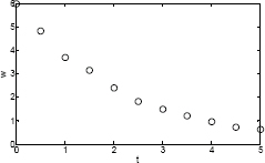

In the left figure, the data points appear to line up along a straight line. This indicates that an exponential function of the form y = bemx can give a good fit to the data. A program in a script file that determines the constants b and m, and that plots the data points and the function is given below.

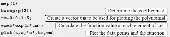
When the program is executed, the values of the constants m and b are displayed in the Command Window.
m =

    -0.4580

b =

    5.9889
The plot generated by the program, which shows the data points and the function (with axis labels added with the Plot Editor) is

It should be pointed out here that in addition to the power, exponential, logarithmic, and reciprocal functions that are discussed in this section, many other functions can be written in a form suitable for curve fitting with the polyfit function. One example where a function of the form y = e(a2x2 + a1x + a0) is fitted to data points using the polyfit function with a third-order polynomial is described in Sample Problem 8-7.
8.3 INTERPOLATION
Interpolation is the estimation of values between data points. MATLAB has interpolation functions that are based on polynomials, which are described in this section, and on Fourier transformation, which is outside the scope of this book. In one-dimensional interpolation, each point has one independent variable (x) and one dependent variable (y). In two-dimensional interpolation, each point has two independent variables (x and y) and one dependent variable (z).
One-dimensional interpolation:
If only two data points exist, the points can be connected with a straight line and a linear equation (polynomial of first order) can be used to estimate values between the points. As was discussed in the previous section, if three (or four) data points exist, a second- (or a third-) order polynomial that passes through the points can be determined and then be used to estimate values between the points. As the number of points increases, a higher-order polynomial is required for the polynomial to pass through all the points. Such a polynomial, however, will not necessarily give a good approximation of the values between the points. This is illustrated in Figure 8-2 with n = 6.
A more accurate interpolation can be obtained if instead of considering all the points in the data set (by using one polynomial that passes through all the points), only a few data points in the neighborhood where the interpolation is needed are considered. In this method, called spline interpolation, many low-order polynomials are used, where each is valid only in a small domain of the data set.
The simplest method of spline interpolation is called linear spline interpolation. In this method, shown on the right, every two adjacent points are connected with a straight line (a polynomial of first degree). The equation of a straight line that passes through two adjacent points (xi, yj) and (xi+1, yj+1) and that can be used to calculate the value of y for any x between the points is given by:

![]()
In a linear interpolation, the line between two data points has a constant slope, and there is a change in the slope at every point. A smoother interpolation curve can be obtained by using quadratic or cubic polynomials. In these methods, called quadratic splines and cubic splines, a second-, or third-order polynomial is used to interpolate between every two points. The coefficients of the polynomial are determined by using data from points that are adjacent to the two data points. The theoretical background for the determination of the constants of the polynomials is beyond the scope of this book and can be found in books on numerical analysis.
One-dimensional interpolation in MATLAB is done with the interp1 (the last character is the numeral one) function, which has the form:

• The vector x must be monotonic (with elements in ascending or descending order).
• xi can be a scalar (interpolation of one point) or a vector (interpolation of many points). yi is a scalar or a vector with the corresponding interpolated values.
• MATLAB can do the interpolation using one of several methods that can be specified. These methods include:
‘nearest’ |
returns the value of the data point that is nearest to the interpolated point. |
‘linear’ |
uses linear spline interpolation. |
‘spline’ |
uses cubic spline interpolation. |
‘pchip’ |
uses piecewise cubic Hermite interpolation, also called ‘cubic’ |
• When the ‘nearest’ and the ‘linear’ methods are used, the value(s) of xi must be within the domain of x. If the ‘spline’ or the ‘pchip’ methods are used, xi can have values outside the domain of x and the function interp1 performs extrapolation.
• The ‘spline’ method can give large errors if the input data points are nonuniform such that some points are much closer together than others.
• Specification of the method is optional. If no method is specified, the default is ‘linear’.
Sample Problem 8-3: Interpolation
The following data points, which are points of the function f(x) = 1.5x cos(2x), are given. Use linear, spline, and pchip interpolation methods to calculate the value of y between the points. Make a figure for each of the interpolation methods. In the figure show the points, a plot of the function, and a curve that corresponds to the interpolation method.

Solution
The following is a program written in a script file that solves the problem:

The three figures generated by the program are shown below (axes labels were added with the Plot Editor). The data points are marked with circles, the interpolation curves are plotted with dashed lines, and the function is shown with a solid line. The left figure shows the linear interpolation, the middle is the spline, and the figure on the right shows the pchip interpolation.

8.4 THE BASIC FITTING INTERFACE
The basic fitting interface is a tool that can be used to perform curve fitting and interpolation interactively. By using the interface the user can:
• Curve-fit the data points with polynomials of various degrees up to 10, and with spline and Hermite interpolation methods.
• Plot the various fits on the same graph so that they can be compared.
• Plot the residuals of the various polynomial fits and compare the norms of the residuals.
• Calculate the values of specific points with the various fits.
• Add the equations of the polynomials to the plot.
To activate the basic fitting interface, the user first has to make a plot of the data points. Then the interface is activated by selecting Basic Fitting in the Tools menu, as shown on the right. This opens the Basic Fitting Window, shown in Figure 8-3. When the window first opens, only one panel (the Plot fits panel) is visible. The window can be extended to show a second panel (the Numerical results panel) by clicking on the ![]() button. One click adds the first section of the panel, and a second click makes the window look as shown in Figure 8-3. The window can be reduced back by clicking on the
button. One click adds the first section of the panel, and a second click makes the window look as shown in Figure 8-3. The window can be reduced back by clicking on the ![]() button. The first two items in the Basic Fitting Window are related to the selection of the data points:
button. The first two items in the Basic Fitting Window are related to the selection of the data points:

Select data: Used to select a specific set of data points for curve fitting in a figure that has more than one set of data points. Only one set of data points can be curve-fitted at a time, but multiple fits can be performed simultaneously on the same set.
Center and scale x data: When this box is checked, the data is centered at zero mean and scaled to unit standard deviation. This might be needed in order to improve the accuracy of numerical computation.
The next four items are in the Plot fits panel and are related to the display of the fit.
Check to display fits on figure: The user selects the fits to be displayed in the figure. The selections include interpolation with spline interpolant (interpolation method) that uses the spline function, interpolation with Hermite interpolant that uses the pchip function, and polynomials of various degrees that use the polyfit function. Several fits can be selected and displayed simultaneously.
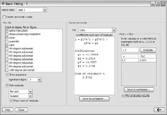
Figure 8-3: The Basic Fitting Window.
Show equations: When this box is checked, the equations of the polynomials that were selected for the fit are displayed in the figure. The equations are displayed with the number of significant digits selected in the adjacent sign menu.
Plot residuals: When this box is checked, a plot that shows the residual at each data point is created (residuals are defined in Section 8.2.1). Choices in the menus include a bar plot, a scatter plot, and a line plot that can be displayed as a subplot in the same Figure Window that has the plot of the data points or as a separate plot in a different Figure Window.
Show norm of residuals: When this box is checked, the norm of the residuals is displayed in the plot of the residuals. The norm of the residual is a measure of the quality of the fit. A smaller norm corresponds to a better fit.
The next three items are in the Numerical results panel. They provide the numerical information for one fit, independently of the fits that are displayed:
Fit: The user selects the fit to be examined numerically. The fit is shown on the plot only if it is selected in the Plot fit panel.
Coefficients and norm of residuals: Displays the numerical results for the polynomial fit that is selected in the Fit menu. It includes the coefficients of the polynomial and the norm of the residuals. The results can be saved by clicking on the Save to workspace button.
Find y = f(x): Provides a means for obtaining interpolated (or extrapolated) numerical values for specified values of the independent variable. Enter the value of the independent variable in the box, and click on the Evaluate button. When the Plot evaluated results box is checked, the point is displayed on the plot.
As an example, the basic fitting interface is used for fitting the data points from Sample Problem 8-3. The Basic Fitting Window is the one shown in Figure 8-3, and the corresponding Figure Window is shown in Figure 8-4. The Figure Window includes a plot of the points, one interpolation fit (spline), two polynomial fits (linear and cubic), a display of the equations of the polynomial fits, and a mark of the point x = 1.5 that is entered in the Find y = f(x) box of the Basic Fitting Window. The Figure Window also includes a plot of the residuals of the polynomial fits and a display of their norm.

Figure 8-4: A Figure Window modified by the Basic Fitting Interface.
8.5 EXAMPLES OF MATLAB APPLICATIONS
Sample Problem 8-4: Determining wall thickness of a box
The outside dimensions of a rectangular box (bottom and four sides, no top), made of aluminum, are 24 by 12 by 4 inches. The wall thickness of the bottom and the sides is x. Derive an expression that relates the weight of the box and the wall thickness x. Determine the thickness x for a box that weighs 15 lb. The specific weight of aluminum is 0.101 lb/in.3.

Solution
The volume of the aluminum VAl is calculated from the weight W of the box by:
![]()
where γ is the specific weight. The volume of the aluminum based on the dimensions of the box is given by
VAl = 24 · 12 · 4 − (24 − 2x)(12 − 2x)(4 − x)
where the inside volume of the box is subtracted from the outside volume. This equation can be rewritten as
(24 − 2x)(12 − 2x)(4 − x) + VAl − (24 · 12 · 4) = 0
which is a third-degree polynomial. A root of this polynomial is the required thickness x. A program in a script file that determines the polynomial and solves for the roots is:

Note in the second-to-last line that in order to add the quantity VAl − (24 · 12 · 4) the polynomial Vin it has to be written as a polynomial of the same order as Vin (Vin is a polynomial of third order). When the program (saved as Chap8SamPro4) is executed, the coefficients of the polynomial and the value of x are displayed:

Sample Problem 8-5: Floating height of a buoy
An aluminum thin-walled sphere is used as a marker buoy. The sphere has a radius of 60 cm and a wall thickness of 12 mm. The density of aluminum is ρAl = 2690 kg/m3. The buoy is placed in the ocean, where the density of the water is 1030 kg/m3. Determine the height h between the top of the buoy and the surface of the water.

Solution
According to Archimedes’s law, the buoyancy force applied to an object that is placed in a fluid is equal to the weight of the fluid that is displaced by the object. Accordingly, the aluminum sphere will be at a depth such that the weight of the sphere is equal to the weight of the fluid displaced by the part of the sphere that is submerged.
The weight of the sphere is given by
![]()
where VAl is the volume of the aluminum; ro and ri are the outside and inside radii of the sphere, respectively; and g is the gravitational acceleration.
The weight of the water that is displaced by the spherical portion that is submerged is given by:
![]()
Setting the two weights equal to each other gives the following equation:
![]()
The last equation is a third-degree polynomial for h. The root of the polynomial is the answer.
A solution with MATLAB is obtained by writing the polynomials and using the roots function to determine the value of h. This is done in the following script file:

When the script file is executed in the Command Window, as shown below, the answer is three roots, since the polynomial is of the third degree. The only answer that is physically possible is the second, where h = 0.9029 m.

Sample Problem 8-6: Determining the size of a capacitor
An electrical capacitor has an unknown capacitance. In order to determine its capacitance, the capacitor is connected to the circuit shown. The switch is first connected to B and the capacitor is charged. Then, the switch is connected to A and the capacitor discharges through the resistor. As the capacitor is discharging, the voltage across the capacitor is measured for 10 s in intervals of 1 s. The recorded measurements are given in the table below. Plot the voltage as a function of time and determine the capacitance of the capacitor by fitting an exponential curve to the data points.


Solution
When a capacitor discharges through a resistor, the voltage of the capacitor as a function of time is given by
V = V0e(−t)/(RC)
where V0 is the initial voltage, R the resistance of the resistor, and C the capacitance of the capacitor. As was explained in Section 8.2.2 the exponential function can be written as a linear equation for ln(V) and t in the form:
![]()
This equation, which has the form y = mx + b, can be fitted to the data points by using the polyfit(x,y,1) function with t as the independent variable x and ln(V) as the dependent variable y. The coefficients m and b determined by the polyfit function are then used to determine C and V0 by:
![]()
The following program written in a script file determines the best-fit exponential function to the data points, determines C and V0, and plots the points and the fitted function.

When the script file is executed (saved as Chap8SamPro6) the values of C and V0 are displayed in the Command Window as shown below:

The program creates also the following plot (axis labels were added to the plot using the Plot Editor):

Sample Problem 8-7: Temperature dependence of viscosity
Viscosity, μ, is a property of gases and fluids that characterizes their resistance to flow. For most materials, viscosity is highly sensitive to temperature. Below is a table that gives the viscosity of SAE 10W oil at different temperatures (data from B.R. Munson, D.F. Young, and T.H. Okiishi, Fundamentals of Fluid Mechanics, 4th ed., John Wiley and Sons, 2002). Determine an equation that can be fitted to the data.
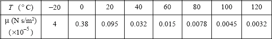
Solution
To determine what type of equation might provide a good fit to the data, μ is plotted as a function of T (absolute temperature) with a linear scale for T and a logarithmic scale for μ. The plot, shown on the right, indicates that the data points do not appear to line up along a straight line. This means that a simple exponential function of the form y = bemx which models a straight line with these axes, will not provide the best fit. Since the points in the figure appear to lie along a curved line, a function that can possibly have a good fit to the data is:
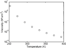
ln(μ) = a2T2 + a1T + a0
This function can be fitted to the data by using MATLAB’s polyfit(x,y,2) function (second-degree polynomial), where the independent variable is T and the dependent variable is ln(μ). The equation above can be solved for μ to give the viscosity as a function of temperature:
![]()
The following program determines the best fit to the function and creates a plot that displays the data points and the function.
T=[-20:20:120];

mu=[4 0.38 0.095 0.032 0.015 0.0078 0.0045 0.0032];

TK=T+273;

p=polyfit(TK,log(mu),2)

Tplot=273+[-20:120];

muplot = exp(p(1) *Tplot. ^2 + p(2) *Tplot + p(3));

semilogy(TK,mu,'o',Tplot,muplot)
When the program executes (saved as Chap8SamPro7), the coefficients that are determined by the polyfit function are displayed in the Command Window (shown below) as three elements of the vector p.
>> Chap8SamPro7

p =

   0.0003 -0.2685 47.1673
With these coefficients the viscosity of the oil as a function of temperature is:
![]()
The plot that is generated shows that the equation correlates well to the data points (axis labels were added with the Plot Editor).

8.6 PROBLEMS
1. Plot the polynomial y = 0.1x5 − 0.2x4 − x3 + 5x2 − 41.5x + 235 in the domain −6 ≤ x ≤ 6. First create a vector for x, next use the polyval function to calculate y, and then use the plot function.
2. Plot the polynomial y = 0.008x4 − 1.8x2 − 5.4x + 54 in the domain −14 ≤ x ≤ 16. First create a vector for x, next use the polyval function to calculate y, and then use the plot function.
3. Use MATLAB to carry out the following multiplication of two polynomials:
(−x3 + 5x − 1)(x4 + 2x3 − 16x + 5)
4. Use MATLAB to carry out the following multiplication of polynomials:
x(x − 1.7)(x + 0.5)(x − 0.7)(x + 1.5)
Plot the polynomial for −1.6 ≤ x ≤ 1.8.
5. Divide the polynomial −10x6 − 20x5 + 9x4 + 10x3 + 8x2 + 11x − 3 by the polynomial 2x2 + 4x − 1.
6. Divide the polynomial
− 0.24x7 + 1.6x6 + 1.5x5 − 7.41x4 − 1.8x3 − 4x2 − 75.2x − 91 by the polynomial − 0.8x3 + 5x + 6.5.
7. The product of two consecutive integers is 6,972. Using MATLAB’s built-in function for operations with polynomials, determine the two integers.
8. The product of three integers with spacing of 5 between them (e.g., 9, 14, 19) is 10,098. Using MATLAB’s built-in function for operations with polynomials, determine the three integers.
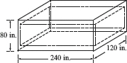
9. A rectangular steel container has the outside dimensions shown in the figure The thickness of the bottom and top walls is t, and the thickness of side walls is t/2. Determine t if the weight of the container is 12,212 lb. The specific weight of steel is 0.284 lb/in3.
10. An aluminum fuel tank has a cylindrical middle section and a semi-spherical ends. The outside diameter is 10 in., and the length of the cylindrical section is 24 in. The wall-thickness of the cylindrical section is t, and the wall-thickness of the semispherical ends is 1.5t. Determine t if the tank weight is 42.27 lb. The specific weight of aluminum is 0.101 lb/in3.

11. A 20 ft−long rod is cut into 12 pieces, which are welded together to form the frame of a rectangular box. The length of the box’s base is 15 in. longer than its width.
(a) Create a polynomial expression for the volume V in terms of x.
(b) Make a plot of V versus x.
(c) Determine the x that maximizes the volume and determine that volume.

12. A rectangular piece of cardboard, 40 in. long by 22 in. wide, is used for making a rectangular box (open top) by cutting out squares of x by x from the corners and folding up the sides.
(a) Create a polynomial expression for the volume V in terms of x.
(b) Make a plot of V versus x.
(c) Determine x if the volume of the box is 1,000 in.3.
(d) Determine the value of x that corresponds to the box with the largest possible volume, and determine that volume.

13. Write a user-defined function that adds or subtracts two polynomials of any order. Name the function p=polyadd(p1,p2,operation). The first two input arguments p1 and p2 are the vectors of the coefficients of the two polynomials. (If the two polynomials are not of the same order, the function adds the necessary zero elements to the shorter vector.) The third input argument operation is a string that can be either ‘add’ or ‘sub’, for adding or subtracting the polynomials, respectively, and the output argument is the resulting polynomial.
Use the function to add and subtract the following polynomials: f1(x) = 2x6 − 3x4 − 9x3 + 11x2 − 8x + 4 and f2(x) = 5x3 + 7x − 10
14. Write a user-defined function that multiplies two polynomials. Name the function p=polymult(p1,p2). The two input arguments p1 and p2 are vectors of the coefficients of the two polynomials. The output argument p is the resulting polynomial.
Use the function to multiply the following polynomials:
f1(x) = 2x6 − 3x4 − 9x3 + 11x2 − 8x + 4 and f2(x) = 5x3 + 7x − 10
Check the answer with MATLAB’s built-in function conv.
15. Write a user-defined function that calculates the maximum (or minimum) of a quadratic equation of the form:
f(x) = ax2 + bx + c
Name the function [x,y,w] = maxormin(a,b,c). The input arguments are the coefficients a, b, and c. The output arguments are x, the coordinate of the maximum (or minimum); y, the maximum (or minimum) value; and w, which is equal to 1 if y is a maximum and equal to 2 if y is a minimum.
Use the function to determine the maximum or minimum of the following functions:
(a) f(x) = 3x2 − 7x + 14
(b) f(x) = − 5x2 − 11x + 15
16. A cone with base radius r and vertex in contact with the surface of a sphere is constructed inside a sphere, as shown in the figure. The radius of the sphere is R = 9 in.
(a) Create a polynomial expression for the volume V of the cone in terms of h.
(b) Make a plot of V versus h for 9 ≤ h ≤ −9.
(c) Using the roots command determine h if the volume of the cone is 500 in.3.
(d) Determine the value of h that corresponds to the cone with the largest possible volume, and determine that volume.

17. Consider the parabola y = 1.5(x − 3)2 + 1 and the point P(3, 5.5).
(a) Create a polynomial expression for the distance d from point P to an arbitrary point Q on the parabola.
(b) Make a plot of d versus x for 3 ≤ x ≤ 6.
(c) Determine the coordinates of Q if d = 28.
(d) Determine the coordinates of Q that correspond to the smallest d, and calculate the corresponding value of d.

18. The following data is given:
![]()
(a) Use linear least-squares regression to determine the coefficients m and b in the function y = mx + b that best fits the data.
(b) Make a plot that shows the function and the data points.
19. The boiling temperature of water TB at various altitudes h is given in the following table. Determine a linear equation in the form TB = mh + b that best fits the data. Use the equation for calculating the boiling temperature at 5,000 m. Make a plot of the points and the equation.

20. The U.S. population in selected years between 1815 and 1965 is listed in the table below. Determine a quadratic equation in the form P = a2t2 + a1t + a0, where t is the number of years after 1800 and P is the population in millions, that best fits the data. Use the equation to estimate the population in 1915 (the population was 98.8 millions). Make a plot of the population versus the year that shows the data points and the equation.

21. The number of bacteria NB measured at different times t is given in the following table. Determine an exponential function in the form NB = Neαt that best fits the data. Use the equation to estimate the number of bacteria after 4.5 hr. Make a plot of the points and the equation.

22. Growth data of a sunflower plant is given in the following table:

The data can be modeled with a function in the form H = C/(1 + Ae−Bt) (logistic equation), where H is the height, C is a maximum value for H, A and B are constants, and t is the number of weeks. By using the method described in Section 8.2.2, and assuming that C = 254 cm, determine the constants A and B such that the function best fit the data. Use the function to estimate the height in week 6. In one figure, plot the function and the data points.
23. Use the growth data from Problem 22 for the following:
(a) Curve-fit the data with a third-order polynomial. Use the polynomial to estimate the height in week 6.
(b) Fit the data with linear and spline interpolations and use each interpolation to estimate the height in week 6.
In each part make a plot of the data points (circle markers) and the fitted curve or the interpolated curves. Note that part (b) has two interpolation curves.
24. The following points are given:
![]()
(a) Fit the data with a first-order polynomial. Make a plot of the points and the polynomial.
(b) Fit the data with a second-order polynomial. Make a plot of the points and the polynomial.
(c) Fit the data with a third-order polynomial. Make a plot of the points and the polynomial.
(d) Fit the data with an fifth-order polynomial. Make a plot of the points and the polynomial.
25. The standard air density, D (average of measurements made), at different heights, h, from sea level up to a height of 33 km is given below.

(a) Make the following four plots of the data points (density as a function of height): (1) both axes with linear scale; (2) h with log axis, D with linear axis; (3) h with linear axis, D with log axis; (4) both log axes. According to the plots choose a function (linear, power, exponential, or logarithmic) that best fits the data points and determine the coefficients of the function.
(b) Plot the function and the points using linear axes.
26. Write a user-defined function that fits data points to a power function of the form y = bxm. Name the function [b,m] = powerfit(x,y), where the input arguments x and y are vectors with the coordinates of the data points, and the output arguments b and m are the constants of the fitted exponential equation. Use powerfit to fit the data below. Make a plot that shows the data points and the function.

27. Viscosity is a property of gases and fluids that characterizes their resistance to flow. For most materials viscosity is highly sensitive to temperature. For gases, the variation of viscosity with temperature is frequently modeled by an equation of the form
![]()
where μ is the viscosity, T is the absolute temperature, and C and S are empirical constants. Below is a table that gives the viscosity of air at different temperatures (data from B.R. Munson, D.F. Young, and T.H. Okiishi, Fundamentals of Fluid Mechanics, 4th ed., John Wiley and Sons, 2002).

Determine the constants C and S by curve-fitting the equation to the data points. Make a plot of viscosity versus temperature (in °C). In the plot show the data points with markers and the curve-fitted equation with a solid line.
The curve fitting can be done by rewriting the equation in the form
![]()
and using a first-order polynomial.
28. Measurements of the fuel efficiency of a car FE at various speeds v are shown in the table.

(a) Curve-fit the data with a second-order polynomial. Use the polynomial to estimate the fuel efficiency at 60 mi/h. Make a plot of the points and the polynomial.
(b) Curve-fit the data with a third-order polynomial. Use the polynomial to estimate the fuel efficiency at 60 mi/h. Make a plot of the points and the polynomial.
(c) Fit the data with linear and spline interpolations. Estimate the fuel efficiency at 60 mi/h with linear and spline interpolations. Make a plot that shows the data points and curves made of interpolated points.
29. The relationship between two variables P and t is known to be:
![]()
The following data points are given
![]()
Determine the constants m and b by curve-fitting the equation to the data points. Make a plot of P versus t. In the plot show the data points with markers and the curve-fitted equation with a solid line. (The curve fitting can be done by writing the reciprocal of the equation and using a first-order polynomial.)
30. When rubber is stretched, its elongation is initially proportional to the applied force, but as it reaches about twice its original length, the force required to stretch the rubber increases rapidly. The force, as a function of elongation, that was required to stretch a rubber specimen that was initially 3 in. long is displayed in the following table.
(a) Curve-fit the data with a forth-order polynomial. Make a plot of the data points and the polynomial. Use the polynomial to estimate the force when the rubber specimen was 11.5 in. long.
(b) Fit the data with spline interpolation (use MATLAB’s built-in function interp1). Make a plot that shows the data points and a curve made by interpolation. Use interpolation to estimate the force when the rubber specimen was 11.5 in. long.

31. The yield strength, σy, of many metals depends on the size of the grains. For these metals, the relationship between the yield stress and the average grain diameter d can be modeled by the Hall-Petch equation:
![]()
The following are results from measurements of average grain diameter and yield stress.
![]()
(a) Using curve fitting, determine the constants σ0 and k in the Hall-Petch equation for this material. Using the constants determine with the equation the yield stress of material with a grain size of 0.05 mm. Make a plot that shows the data points with circle markers and the curve derived from the Hall-Petch equation with a solid line.
(b) Use linear interpolation to determine the yield stress of material with a grain size of 0.05 mm. Make a plot that shows the data points with circle markers and the linear interpolation with a solid line.
(c) Use cubic interpolation to determine the yield stress of material with a grain size of 0.05 mm. Make a plot that shows the data points with circle markers and cubic interpolation with a solid line.
32. The transmission of light through a transparent solid can be described by the equation:
![]()
where IT is the transmitted intensity, I0 is the intensity of the incident beam, β is the absorption coefficient, L is the length of the transparent solid, and R is the fraction of light which is reflected at the interface. If the light is normal to the interface and the beams are transmitted through air, ![]() where n is the index of refraction for the transparent solid. Experiments measuring the intensity of light transmitted through specimens of a transparent solid of various lengths are given in the following table. The intensity of the incident beam is 5 watts/m2.
where n is the index of refraction for the transparent solid. Experiments measuring the intensity of light transmitted through specimens of a transparent solid of various lengths are given in the following table. The intensity of the incident beam is 5 watts/m2.

Use this data and curve fitting to determine the absorption coefficient and index of refraction of the solid.
33. The ideal gas equation relates the volume, pressure, temperature, and the quantity of a gas by:
![]()
where V is the volume in liters, P is the pressure in atm, T is the temperature in kelvins, n is the number of moles, and R is the gas constant.
An experiment is conducted for determining the value of the gas constant R. In the experiment, 0.05 mol of gas is compressed to different volumes by applying pressure to the gas. At each volume, the pressure and temperature of the gas are recorded. Using the data given below, determine R by plotting V versus T/P and fitting the data points with a linear equation.
