Chapter 7

User-Defined Functions and Function Files

A simple function in mathematics, f(x), associates a unique number to each value of x. The function can be expressed in the form y = f(x), where f(x) is usually a mathematical expression in terms of x. A value of y (output) is obtained when a value of x (input) is substituted in the expression. Many functions are programmed inside MATLAB as built-in functions, and can be used in mathematical expressions simply by typing their name with an argument (see Section 1.5); examples are sin(x), cos(x), sqrt(x), and exp(x). Frequently, in computer programs, there is a need to calculate the value of functions that are not built in. When a function expression is simple and needs to be calculated only once, it can be typed as part of the program. However, when a function needs to be evaluated many times for different values of arguments, it is convenient to create a “user-defined” function. Once a user-defined function is created (saved) it can be used just like the built-in functions.

A user-defined function is a MATLAB program that is created by the user, saved as a function file, and then used like a built-in function. The function can be a simple single mathematical expression or a complicated and involved series of calculations. In many cases it is actually a subprogram within a computer program. The main feature of a function file is that it has an input and an output. This means that the calculations in the function file are carried out using the input data, and the results of the calculations are transferred out of the function file by the output. The input and the output can be one or several variables, and each can be a scalar, a vector, or an array of any size. Schematically, a function file can be illustrated by:

A very simple example of a user-defined function is a function that calculates the maximum height that a ball reaches when thrown upward with a certain velocity. For a velocity v₀, the maximum height h_max is given by , where g is the gravitational acceleration. In function form this can be written as . In this case the input to the function is the velocity (a number), and the output is the maximum height (a number). For example, in SI units (g = 9.81 m/s²) if the input is 15 m/s, the output is 11.47 m.

In addition to being used as math functions, user-defined functions can be used as subprograms in large programs. In this way large computer programs can be made up of smaller “building blocks” that can be tested independently. Function files are similar to subroutines in Basic and Fortran, procedures in Pascal, and functions in C.

The fundamentals of user-defined functions are explained in Sections 7.1 through 7.7. In addition to user-defined functions that are saved in separate function files and called for use in a computer program, MATLAB provides an option to define and use a user-defined math function within a computer program (not in a separate file). This can be done by using anonymous function, which is presented in Section 7.8. There are built-in and user-defined functions that have to be supplied with other functions when they are called. These functions, which in MATLAB are called function functions, are introduced in Section 7.9. The last two sections cover subfunctions and nested functions. Both are methods for incorporating two or more user-defined functions in a single function file.

7.1 CREATING A FUNCTION FILE

Function files are created and edited, like script files, in the Editor/Debugger Window. This window is opened from the Command Window. In the Toolstrip select New, then select Function. Once the Editor/Debugger Window opens, it looks like that shown in Figure 7-1. The editor contains several pre-typed lines that outline the structure of a function file. The first line is the function definition line, which is followed by comments the describe the function. Next comes the program (the empty lines 4 and 5 in Figure 7-1), and the last line is an end statement, which is optional. The structure of a function file is described in detail in the next section.

Note: The Editor/Debugger Window can also be opened (as was described in Chapter 1) by clicking on the New Script icon in the Toolstrip, or by clicking New in the Toolstrip and then selecting Script from the menu that open. The window that opens is empty, without any pre-typed lines. In general, the Editor/Debugger Window can be used for writing a script file or a function file.

Figure 7-1: The Editor/Debugger Window.

7.2 STRUCTURE OF A FUNCTION FILE

The structure of a typical complete function file is shown in Figure 7-2. This particular function calculates the monthly payment and the total payment of a loan. The inputs to the function are the amount of the loan, the annual interest rate, and the duration of the loan (number of years). The output from the function is the monthly payment and the total payment.

Figure 7-2: Structure of a typical function file.

The various parts of the function file are described in detail in the following sections.

7.2.1 Function Definition Line

The first executable line in a function file must be the function definition line. Otherwise the file is considered a script file. The function definition line:

•   Defines the file as a function file

•   Defines the name of the function

•   Defines the number and order of the input and output arguments

The form of the function definition line is:

The word “function,” typed in lowercase letters, must be the first word in the function definition line. On the screen the word function appears in blue. The function name is typed following the equal sign. The name can be made up of letters, digits, and the underscore character (the name cannot include a space). The rules for the name are the same as the rules for naming variables described in Section 1.6.2. It is good practice to avoid names of built-in functions and names of variables already defined by the user or predefined by MATLAB.

7.2.2 Input and Output Arguments

The input and output arguments are used to transfer data into and out of the function. The input arguments are listed inside parentheses following the function name. Usually, there is at least one input argument, although it is possible to have a function that has no input arguments. If there are more than one, the input arguments are separated with commas. The computer code that performs the calculations within the function file is written in terms of the input arguments and assumes that the arguments have assigned numerical values. This means that the mathematical expressions in the function file must be written according to the dimensions of the arguments, since the arguments can be scalars, vectors, or arrays. In the example shown in Figure 7-2 there are three input arguments (amount,rate,years), and in the mathematical expressions they are assumed to be scalars. The actual values of the input arguments are assigned when the function is used (called). Similarly, if the input arguments are vectors or arrays, the mathematical expressions in the function body must be written to follow linear algebra or element-by-element calculations.

The output arguments, which are listed inside brackets on the left side of the assignment operator in the function definition line, transfer the output from the function file. Function files can have zero, one, or several output arguments. If there are more than one, the output arguments are separated with commas. If there is only one output argument, it can be typed without brackets. For the function file to work, the output arguments must be assigned values in the computer program that is in the function body. In the example in Figure 7-2 there are two output arguments, mpay and tpay. When a function does not have an output argument, the assignment operator in the function definition line can be omitted. A function without an output argument can, for example, generate a plot or write data to a file.

It is also possible to transfer strings into a function file. This is done by typing the string as part of the input variables (text enclosed in single quotes). Strings can be used to transfer names of other functions into the function file.

Usually, all the input to, and the output from, a function file transferred through the input and output arguments. In addition, however, all the input and output features of script files are valid and can be used in function files. This means that any variable that is assigned a value in the code of the function file will be displayed on the screen unless a semicolon is typed at the end of the command. In addition, the input command can be used to input data interactively, and the disp, fprintf, and plot commands can be used to display information on the screen, save to a file, or plot figures just as in a script file. The following are examples of function definition lines with different combinations of input and output arguments.

Function definition line	Comments
function [mpay,tpay] = loan(amount,rate,years)	Three input arguments, two output arguments.
function [A] = RectArea(a,b)	Two input arguments, one output argument.
function A = RectArea(a,b)	Same as above; one output argument can be typed without the brackets.
function [V, S] = SphereVolArea(r)	One input variable, two output variables.
function trajectory(v,h,g)	Three input arguments, no output arguments.

7.2.3 The H1 Line and Help Text Lines

The H1 line and help text lines are comment lines (lines that begin with the percent, %, sign) following the function definition line. They are optional but are frequently used to provide information about the function. The H1 line is the first comment line and usually contains the name and a short definition of the function. When a user types (in the Command Window) lookfor a_word, MATLAB searches for a_word in the H1 lines of all the functions, and if a match is found, the H1 line that contains the match is displayed.

The help text lines are comment lines that follow the H1 line. These lines contain an explanation of the function and any instructions related to the input and output arguments. The comment lines that are typed between the function definition line and the first non-comment line (the H1 line and the help text) are displayed when the user types help function_name in the Command Window. This is true for MATLAB built-in functions as well as the user-defined functions. For example, for the function loan in Figure 7-2, if help loan is typed in the Command Window (make sure the current directory or the search path includes the directory where the file is saved), the display on the screen is:

A function file can include additional comment lines in the function body. These lines are ignored by the help command.

7.2.4 Function Body

The function body contains the computer program (code) that actually performs the computations. The code can use all MATLAB programming features. This includes calculations, assignments, any built-in or user-defined functions, flow control (conditional statements and loops) as explained in Chapter 6, comments, blank lines, and interactive input and output.

7.3 LOCAL AND GLOBAL VARIABLES

All the variables in a function file are local (the input and output arguments and any variables that are assigned values within the function file). This means that the variables are defined and recognized only inside the function file. When a function file is executed, MATLAB uses an area of memory that is separate from the workspace (the memory space of the Command Window and the script files). In a function file the input variables are assigned values each time the function is called. These variables are then used in the calculations within the function file. When the function file finishes its execution, the values of the output arguments are transferred to the variables that were used when the function was called. All this means that a function file can have variables with the same names as variables in the Command Window or in script files. The function file does not recognize variables with the same names as have been assigned values outside the function. The assignment of values to these variables in the function file will not change their assignment elsewhere.

Each function file has its own local variables, which are not shared with other functions or with the workspace of the Command Window and the script files. It is possible, however, to make a variable common (recognized) in several different function files, and perhaps in the workspace too. This is done by declaring the variable global with the global command, which has the form:

Several variables can be declared global by listing them, separated with spaces, in the global command. For example:

global GRAVITY_CONST FrictionCoefficient

•   The variable has to be declared global in every function file that the user wants it to be recognized in. The variable is then common only to these files.

•   The global command must appear before the variable is used. It is recommended to enter the global command at the top of the file.

•   The global command has to be entered in the Command Window, or in a script file, for the variable to be recognized in the workspace.

•   The variable can be assigned, or reassigned, a value in any of the locations in which it is declared common.

•   The use of long descriptive names (or all capital letters) is recommended for global variables in order to distinguish them from regular variables.

7.4 SAVING A FUNCTION FILE

A function file must be saved before it can be used. This is done, as with a script file, by choosing Save as . . . from the File menu, selecting a location (many students save to a flash drive), and entering the file name. It is highly recommended that the file be saved with a name that is identical to the function name in the function definition line. In this way the function is called (used) by using the function name. (If a function file is saved with a different name, the name it is saved under must be used when the function is called.) Function files are saved with the extension .m. Examples:

Function definition line	File name
function [mpay,tpay] = loan(amount,rate,years)	loan.m
function [A] = RectArea(a,b)	RectArea.m
function [V, S] = SphereVolArea(r)	SphereVolArea.m
function trajectory(v,h,g)	trajectory.m

7.5 USING A USER-DEFINED FUNCTION

A user-defined function is used in the same way as a built-in function. The function can be called from the Command Window, from a script file, or from another function. To use the function file, the folder where it is saved must either be in the current folder or be in the search path (see Sections 1.8.3 and 1.8.4).

A function can be used by assigning its output to a variable (or variables), as a part of a mathematical expression, as an argument in another function, or just by typing its name in the Command Window or in a script file. In all cases the user must know exactly what the input and output arguments are. An input argument can be a number, a computable expression, or a variable that has an assigned value. The arguments are assigned according to their position in the input and output argument lists in the function definition line.

Two of the ways that a function can be used are illustrated below with the user-defined loan function in Figure 7-2, which calculates the monthly and total payments (two output arguments) of a loan. The input arguments are the loan amount, annual interest rate, and the length (number of years) of the loan. In the first illustration the loan function is used with numbers as input arguments:

In the second illustration the loan function is used with two pre-assigned variables and a number as the input arguments:

7.6 EXAMPLES OF SIMPLE USER-DEFINED FUNCTIONS

Sample Problem 7-1:   User-defined function for a math function

Write a function file (name it chp7one) for the function . The input to the function is x and the output is f(x). Write the function such that x can be a vector. Use the function to calculate:

(a) f(x) for x = 6.

(b) f(x) for x = 1, 3, 5, 7, 9, and 11.

Solution

The function file for the function f(x) is:

Note that the mathematical expression in the function file is written for element-by-element calculations. In this way if x is a vector, y will also be a vector. The function is saved and then the search path is modified to include the directory where the file was saved. As shown below, the function is used in the Command Window.

(a) Calculating the function for x = 6 can be done by typing chp7one(6) in the Command Window, or by assigning the value of the function to a new variable:

(b) To calculate the function for several values of x, a vector with the values of x is created and then used for the argument of the function.

Another way is to type the vector x directly in the argument of the function.

Sample Problem 7-2:   Converting temperature units

Write a user-defined function (name it FtoC) that converts temperature in degrees F to temperature in degrees C. Use the function to solve the following problem. The change in the length of an object, ΔL, due to a change in the temperature, ΔT, is given by: ΔL = αLΔT, where α is the coefficient of thermal expansion. Determine the change in the area of a rectangular (4.5 m by 2.25 m) aluminum (α = 23 · 10⁻⁶ 1/°C) plate if the temperature changes from 40° F to 92° F.

Solution

A user-defined function that converts degrees F to degrees C is:

A script file (named Chapter7Example2) that calculates the change of the area of the plate due to the temperature is:

Executing the script file in the Command Window gives the solution:

7.7 COMPARISON BETWEEN SCRIPT FILES AND FUNCTION FILES

Students who are studying MATLAB for the first time sometimes have difficulty understanding exactly the differences between script and function files, since for many of the problems that they are asked to solve using MATLAB, either type of file can be used. The similarities and differences between script and function files are summarized below.

•   Both script and function files are saved with the extension .m (that is why they are sometimes called M-files).

•   The first executable line in a function file is (must be) the function definition line.

•   The variables in a function file are local. The variables in a script file are recognized in the Command Window.

•   Script files can use variables that have been defined in the workspace.

•   Script files contain a sequence of MATLAB commands (statements).

•   Function files can accept data through input arguments and can return data through output arguments.

•   When a function file is saved, the name of the file should be the same as the name of the function.

•   A user-defined function is used in the same way as a built-in function. It can be used (called) in the Command Window, in a script file, or in another function.

7.8 ANONYMOUS FUNCTIONS

User-defined functions written in function files can be used for simple mathematical functions, for large and complicated math functions that require extensive programming, and as subprograms in large computer programs. In cases when the value of a relatively simple mathematical expression has to be calculated many times within a program, MATLAB provides the option of using anonymous functions. An anonymous function is a user-defined function that is defined and written within the computer code (not in a separate function file) and is then used in the code. Anonymous functions can be defined in any part of MATLAB (in the Command Window, in script files, and inside regular user-defined functions).

An anonymous function is a simple (one-line) user-defined function that is defined without creating a separate function file (m-file). Anonymous functions can be constructed in the Command Window, within a script file, or inside a regular user-defined function.

An anonymous function is created by typing the following command:

A simple example is cube = @ (x) x^3, which calculates the cube of the input argument.

•   The command creates the anonymous function and assigns a handle for the function to the variable name on the left-hand side of the = sign. (Function handles provide means for using the function and passing it to other functions; see Section 7.9.1.)

•   The expr consists of a single valid mathematical MATLAB expression.

•   The mathematical expression can have one or several independent variables. The independent variable(s) is (are) entered in the (arglist). Multiple independent variables are separated with commas. An example of an anonymous function that has two independent variables is: circle = @ (x,y) 16*x^2+9*y^2

•   The mathematical expression can include any built-in or user-defined functions.

•   The expression must be written according to the dimensions of the arguments (element-by-element or linear algebra calculations).

•   The expression can include variables that are already defined when the anonymous function is defined. For example, if three variables a, b, and c are defined (have assigned numerical values), then they can be used in the expression of the anonymous function parabola = @ (x) a*x^2+b*x+c.

Important note: MATLAB captures the values of the predefined variables when the anonymous function is defined. This means that if new values are subsequently assigned to the predefined variables, the anonymous function is not changed. The anonymous function has to be redefined in order for the new values of the predefined variables to be used in the expression.

Using an anonymous function:

•   Once an anonymous function is defined, it can be used by typing its name and a value for the argument (or arguments) in parentheses (see examples that follow).

•   Anonymous functions can also be used as arguments in other functions (see Section 7.9.1).

Example of an anonymous function with one independent variable:

The function can be defined (in the Command Window) as an anonymous function for x as a scalar by:

If a semicolon is not typed at the end, MATLAB responds by displaying the function. The function can then be used for different values of x, as shown below.

If x is expected to be an array, with the function calculated for each element, then the function must be modified for element-by-element calculations.

Example of an anonymous function with several independent variables:

The function f(x, y) = 2x² − 4xy + y² can be defined as an anonymous function by:

Then the anonymous function can be used for different values of x and y. For example, typing HA(2,3) gives:
Another example of using an anonymous function with several arguments is shown in Sample Problem 6-3.

Sample Problem 7-3:   Distance between points in polar coordinates

Write an anonymous function that calculates the distance between two points in a plane when the position of the points is given in polar coordinates. Use the anonymous function to calculate the distance between point A (2, π/6) and point B (5, 3π/4).

Solution

The distance between two points in polar coordinates can be calculated by using the Law of Cosines:

The formula for the distance is entered as an anonymous function with four input arguments (r_A, θ_A, r_B, θ_B). Then the function is used for calculating the distance between points A and B.

7.9 FUNCTION FUNCTIONS

There are many situations where a function (Function A) works on (uses) another function (Function B). This means that when Function A is executed, it has to be provided with Function B. A function that accepts another function is called in MATLAB a function function. For example, MATLAB has a built-in function called fzero (Function A) that finds the zero of a math function (Function B) — i.e., the value of x where f(x) = 0. The program in the function fzero is written such that it can find the zero of any f(x). When fzero is called, the specific function to be solved is passed into fzero, which finds the zero of the f(x). (The function fzero is described in detail in Chapter 9.)

A function function, which accepts another function (imported function), includes in its input arguments a name that represents the imported function. The imported function name is used for the operations in the program (code) of the function function. When the function function is used (called), the specific function that is imported is listed in its input argument. In this way different functions can be imported (passed) into the function function. There are two methods for listing the name of an imported function in the argument list of a function function. One is by using a function handle (Section 7.9.1), and the other is by typing the name of the function that is being passed in as a string expression (Section 7.9.2). The method that is used affects the way that the operations in the function function are written (this is explained in more detail in the next two sections). Using function handles is easier and more efficient, and should be the preferred method.

7.9.1 Using Function Handles for Passing a Function into a Function Function

Function handles are used for passing (importing) user-defined functions, built-in functions, and anonymous functions into function functions that can accept them. This section first explains what a function handle is, then shows how to write a user-defined function function that accepts function handles, and finally shows how to use function handles for passing functions into function functions.

Function handle:

A function handle is a MATLAB value that is associated with a function. It is a MATLAB data type and can be passed as an argument into another function. Once passed, the function handle provides means for calling (using) the function it is associated with. Function handles can be used with any kind of MATLAB function. This includes built-in functions, user-defined functions (written in function files), and anonymous functions.

•   For built-in and user-defined functions, a function handle is created by typing the symbol @ in front of the function name. For example, @cos is the function handle of the built-in function cos, and @FtoC is the function handle of the user-defined function FtoC that was created in Sample Problem 7-2.

•   The function handle can also be assigned to a variable name. For example, cosHandle=@cos assigns the handle @cos to cosHandle. Then the name cosHandle can be used for passing the handle.

•   As anonymous functions (see Section 7.8.1), their name is already a function handle.

Writing a function function that accepts a function handle as an input argument:

As already mentioned, the input arguments of a function function (which accepts another function) includes a name (dummy function name) that represents the imported function. This dummy function (including a list of input arguments enclosed in parentheses) is used for the operations of the program inside the function function.

•   The function that is actually being imported must be in a form consistent with the way that the dummy function is being used in the program. This means that both must have the same number and type of input and output arguments.

The following is an example of a user-defined function function, named funplot, that makes a plot of a function (any function f(x) that is imported into it) between the points x = a and x = b. The input arguments are (Fun,a,b), where Fun is a dummy name that represents the imported function, and a and b are the end points of the domain. The function funplot also has a numerical output xyout, which is a 3 × 2 matrix with the values of x and f(x) at the three points x = a, x = (a + b)/2, and x = b. Note that in the program, the dummy function Fun has one input argument (x) and one output argument y, which are both vectors.

As an example, the function f(x) = e^−0.17xx³ − 2x² + 0.8x − 3 over the domain [0.5, 4] is passed into the user-defined function funplot. This is done in two ways: first by writing a user-defined function for f(x), and then by writing f(x) as an anonymous function.

Passing a user-defined function into a function function:

First, a user-defined function is written for f(x). The function, named Fdemo, calculates f(x) for a given value of x and is written using element-by-element operations.

Next, the function Fdemo is passed into the user-defined function function funplot, which is called in the Command Window. Note that a handle of the user-defined function Fdemo is entered (the handle is @Fdemo) for the input argument Fun in the user-defined function funplot.

In addition to the display of the numerical output, when the command is executed, the plot shown in Figure 7-3 is displayed in the Figure Window.

Figure 7-3: A plot of the function f(x) = e^−0.17xx³ − 2x² + 0.8x − 3.

Passing an anonymous function into a function function:

To use an anonymous function, the function f(x) = e^−0.17xx³ − 2x² + 0.8x − 3 first has to be written as an anonymous function, and then passed into the user-defined function funplot. The following shows how both of these steps are done in the Command Window. Note that the name of the anonymous function FdemoAnony is entered without the @ sign for the input argument Fun in the user-defined function funplot (since the name is already the handle of the anonymous function).

In addition to the display of the numerical output in the Command Window, the plot shown in Figure 7-3 is displayed in the Figure Window.

7.9.2 Using a Function Name for Passing a Function into a Function Function

A second method for passing a function into a function function is by typing the name of the function that is being imported as a string in the input argument of the function function. The method that was used before the introduction of function handles can be used for importing user-defined functions. As mentioned, function handles are easier to use and more efficient and should be the preferred method. Importing user-defined functions by using their name is covered in the present edition of the book for the benefit of readers who need to understand programs written before MATLAB 7. New programs should use function handles.

When a user-defined function is imported by using its name, the value of the imported function inside the function function has to be calculated with the feval command. This is different from the case where a function handle is used, which means that there is a difference in the way that the code in the function function is written that depends on how the imported function is passed in.

The feval command:

The feval (short for “function evaluate”) command evaluates the value of a function for a given value (or values) of the function’s argument (or arguments). The format of the command is:

The value that is determined by feval can be assigned to a variable, or if the command is typed without an assignment, MATLAB displays ans = and the value of the function.

•   The function name is typed as string.

•   The function can be a built-in or a user-defined function.

•   If there is more than one input argument, the arguments are separated with commas.

•   If there is more than one output argument, the variables on the left-hand side of the assignment operator are typed inside brackets and separated with commas.

Two examples using the feval command with built-in functions follow.

The following shows the use of the feval command with the user-defined function loan that was created earlier in the chapter (Figure 7-2). This function has three input arguments and two output arguments.

Writing a function function that accepts a function by typing its name as an input argument:

As already mentioned, when a user-defined function is imported by using its name, the value of the function inside the function function has to be calculated with the feval command. This is demonstrated in the following user-defined function function that is called funplotS. The function is the same as the function funplot from Section 7.9.1, except that the command feval is used for the calculations with the imported function.

Passing a user-defined function into another function by using a string expression:

The following demonstrates how to pass a user-defined function into a function function by typing the name of the imported function as a string in the input argument. The function f(x) = e^−0.17xx³ − 2x² + 0.8x − 3 from Section 7.9.1, created as a user-defined function named Fdemo, is passed into the user-defined function funplotS. Note that the name Fdemo is typed in a string for the input argument Fun in the user-defined function funplotS.

In addition to the display of the numerical output in the Command Window, the plot shown in Figure 7-3 is displayed in the Figure Window.

7.10 SUBFUNCTIONS

A function file can contain more than one user-defined function. The functions are typed one after the other. Each function begins with a function definition line. The first function is called the primary function and the rest of the functions are called subfunctions. The subfunctions can be typed in any order. The name of the function file that is saved should correspond to the name of the primary function. Each of the functions in the file can call any of the other functions in the file. Outside functions, or programs (script files), can call only the primary function. Each of the functions in the file has its own workspace, which means that in each the variables are local. In other words, the primary function and the subfunctions cannot access each other’s variables (unless variables are declared to be global).

Subfunctions can help in writing user-defined functions in an organized manner. The program in the primary function can be divided into smaller tasks, each of which is carried out in a subfunction. This is demonstrated in Sample Problem 7-4.

Sample Problem 7-4:   Average and standard deviation

Write a user-defined function that calculates the average and the standard deviation of a list of numbers. Use the function to calculate the average and the standard deviation of the following list of grades:
80  75  91  60  79  89  65  80  95  50  81

Solution

The average x_ave (mean) of a given set of n numbers x₁, x₂, …, x_n is given by:

x_ave = (x₁ + x₂ + … + x_n)/n

The standard deviation is given by:

A user-defined function, named stat, is written for solving the problem. To demonstrate the use of subfunctions, the function file includes stat as a primary function, and two subfunctions called AVG and StandDiv. The function AVG calculates x_ave, and the function StandDiv calculates σ. The subfunctions are called by the primary function. The following listing is saved as one function file called stat.

The user-defined function stat is then used in the Command Window for calculating the average and the standard deviation of the grades:

7.11 NESTED FUNCTIONS

A nested function is a user-defined function that is written inside another user-defined function. The portion of the code that corresponds to the nested function starts with a function definition line and ends with an end statement. An end statement must also be entered at the end of the function that contains the nested function. (Normally, a user-defined function does not require a terminating end statement. However, an end statement is required if the function contains one or more nested functions.) Nested functions can also contain nested functions. Obviously, having many levels of nested functions can be confusing. This section considers only two levels of nested functions.

One nested function:

The format of a user-defined function A (called the primary function) that contains one nested function B is:

•   Note the end statements at the ends of functions B and A.

•   The nested function B can access the workspace of the primary function A, and the primary function A can access the workspace of the function B. This means that a variable defined in the primary function A can be read and redefined in nested function B and vice versa.

•   Function A can call function B, and function B can call function A.

Two (or more) nested functions at the same level:

The format of a user-defined function A (called the primary function) that contains two nested functions B and C at the same level is:

•   The three functions can access the workspace of each other.

•   The three functions can call each other.

As an example, the following user-defined function (named statNest), with two nested functions at the same level, solves Sample Problem 7-4. Note that the nested functions are using variables (n and me) that are defined in the primary function.

Using the user-defined function statNest in the Command Window for calculating the average of the grade data gives:

Two levels of nested functions:

Two levels of nested functions are created when nested functions are written inside nested functions. The following shows an example for the format of a user-defined function with four nested functions in two levels.

The following rules apply to nested functions:

•   A nested function can be called from a level above it. (In the preceding example, function A can call B or D, but not C or E.)

•   A nested function can be called from a nested function at the same level within the primary function. (In the preceding example, function B can call D, and D can call B.)

•   A nested function can be called from a nested function at any lower level.

•   A variable defined in the primary function is recognized and can be redefined by a function that is nested at any level within the primary function.

•   A variable defined in a nested function is recognized and can be redefined by any of the functions that contain the nested function.

7.12 EXAMPLES OF MATLAB APPLICATIONS

Sample Problem 7-5:   Exponential growth and decay

A model for exponential growth or decay of a quantity is given by

A(t) = A₀e^kt

where A(t) and A₀ are the quantity at time t and time 0, respectively, and k is a constant unique to the specific application.

Write a user-defined function that uses this model to predict the quantity A(t) at time t from knowledge of A₀ and A(t₁) at some other time t₁. For function name and arguments, use At = expGD(A0,At1,t1,t), where the output argument At corresponds to A(t), and for input arguments, use A0,At1,t1,t, corresponding to A₀, A(t₁), t₁, and t, respectively.

Use the function file in the Command Window for the following two cases:

(a) The population of Mexico was 67 million in the year 1980 and 79 million in 1986. Estimate the population in 2000.

(b) The half-life of a radioactive material is 5.8 years. How much of a 7-gram sample will be left after 30 years?

Solution

To use the exponential growth model, the value of the constant k has to be determined first by solving for k in terms of A₀, A(t₁), and t₁:

Once k is known, the model can be used to estimate the population at any time.

The user-defined function that solves the problem is:

Once the function is saved, it is used in the Command Window to solve the two cases. For case a) A₀ = 67, A(t₁) = 79, t₁ = 6, and t = 20:

For case b) A₀ = 7, A(t₁) = 3.5 (since t₁ corresponds to the half-life, which is the time required for the material to decay to half of its initial quantity), t₁ = 5.8, and t = 30.

Sample Problem 7-6:   Motion of a projectile

Create a function file that calculates the trajectory of a projectile. The inputs to the function are the initial velocity and the angle at which the projectile is fired. The outputs from the function are the maximum height and distance. In addition, the function generates a plot of the trajectory. Use the function to calculate the trajectory of a projectile that is fired at a velocity of 230 m/s at an angle of 39°.

Solution

The motion of a projectile can be analyzed by considering the horizontal and vertical components. The initial velocity v₀ can be resolved into horizontal and vertical components

In the vertical direction the velocity and position of the projectile are given by:

The time it takes the projectile to reach the highest point (v_y = 0) and the corresponding height are given by:

The total flying time is twice the time it takes the projectile to reach the highest point, t_tot = 2t_hmax. In the horizontal direction the velocity is constant, and the position of the projectile is given by:

x = v_0xt

In MATLAB notation the function name and arguments are entered as [hmax,dmax] = trajectory(v0,theta). The function file is:

After the function is saved, it is used in the Command Window for a projectile that is fired at a velocity of 230 m/s and an angle of 39°.

In addition, the following figure is created in the Figure Window:

7.13 PROBLEMS

1. Write a user-defined MATLAB function for the following math function:

y(x) = (−0.2x³ + 7x²)e^−0.3x

The input to the function is x and the output is y. Write the function such that x can be a vector (use element-by-element operations).

(a) Use the function to calculate y(−1.5) and y(5).

(b) Use the function to make a plot of the function y(x) for −2 ≤ x ≤ 6.

2. Write a user-defined MATLAB function for the following math function:

r(θ) = 4cos(4 sinθ)

The input to the function is θ (in radians) and the output is r. Write the function such that θ can be a vector.

(a) Use the function to calculate r(π/6) and r(5π/6).

(b) Use the function to plot (polar plot) r(θ) for 0 ≤ θ ≤ 2π.

3. The fuel consumption of an airplane is measured in gal/mi (gallon per mile) or in L/km (liter per kilometers). Write a MATLAB user-defined function that converts fuel efficiency consumption from gal/mi to L/km. For the function name and arguments, use Lkm=LkmToGalm(gmi). The input argument gmi is the consumption in gal/mi, and the output argument Lkm is the consumption in L/km. Use the function in the Command Window to:

(a) Determine the fuel consumption in L/km of a Boeing 747 whose fuel consumption is about 5 gal/mi.

(b) Determine the fuel consumption in L/km of the Concorde whose fuel consumption is about 5.8 gal/mi.

4. Tables of materials properties list density, in units of kg/m³, when the international system of units (SI) is used and list specific weight, in units of lb/in³, when the U.S. customary system of units are used. Write a user-defined MATLAB function that converts density to specific weight. For the function name and arguments, use [sw] = DenToSw(den). The input argument den is the density of a material in kg/m³, and the output argument sw is the specific weight in lb/in³. Use the function in the Command Window to:

(a) Determine the specific weight of steel whose density is 7860 kg/m³

(b) Determine the specific weight of titanium whose density is 4730 kg/m³

5. Write a user-defined MATLAB function that converts speed given in units of knots (one knot is one nautical mile per hour) to speed in units of feet per second. For the function name and arguments, use fps = ktsTOfps(kts). The input argument kts is the speed in knots, and the output argument fps is the speed in ft/s. Use the function to convert 400 kts to units of ft/s.

6. The body surface area (BSA) in m² of a person (used for determining dosage of medications) can be calculated by the formula (Du Bois formula):

BSA = 0.007184W^0.425 H^0.75

in which W is the mass in kg and H is the height in cm.

Write a MATLAB user-defined function that calculates the body surface area. For the function name and arguments, use BSA = BodySurA(w,h). The input arguments w and h are the mass and height, respectively. The output argument BSA is the BSA value. Use the function to calculate the body surface area of:

(a) A 95 kg, 1.87 m person.

(b) A 61 kg, 1.58 m person.

7. The fuel tank shown in the figure in shaped as a frustum of cone with r = 20 in., and H = 2r.

Write a user-defined function (for the function name and arguments, use V = Volfuel(y)) that gives the volume of fuel in the tank (in gallons) as a function of the height y (measured from the bottom). Use the function to make a plot of the volume as a function of h for 0 ≤ h ≤ 40 in.

8. The surface area S of a ring in shape of a torus with an inner radius r and a diameter d is given by:

S = π²(2r + d)d

The ring is to be plated with a thin layer of coating. The weight of the coating W can be calculated approximately as W = γSt, where γ is the specific weight of the coating material and t is its thickness. Write an anonymous function that calculates the weight of the coating. The function should have four input arguments, r, d, t, and γ. Use the anonymous function to calculate the weight of a gold coating (γ = 0.696 lb/in.³) of a ring with r = 0.35 in., d = 0.12 in., and t = 0.002 in.

9. The windchill temperature T_WC is the perceived air temperature felt by the body on exposed skin due to the flow of air. For temperatures below 50° F and wind speed higher than 3 mph, it is calculated by:

T_WC = C₁ + C₂T_A + C₃ V^0.16 + C₄T_AV^0.16

where T_A is the air temperature in degrees F, V is the wind speed in mph, C₁ = 35.74, C₂ = 0.6215, C₃ = −35.75, and C₄ = 0.4275. Write a user-defined function for calculating T_WC for given T_A and V. For the function name and arguments, use Twc=WindChill(T,V). The input arguments are T the air temperature in °F and V the wind speed in mph, respectively. The output argument is Twc, the windchill temperature in °F (rounded to the nearest integer). Use the function to determine the windchill temperature for the following conditions:

(a) T = 35 °F, V = 26 mph.

(b) T = 10 °F, V = 50 mph.

10. Write a user-defined function that calculates grade point average (GPA) on a scale of 0 to 4, where A = 4, A− = 3.7, B+ = 3.3, B = 3, B− = 2.7, C+ = 2.3, C = 2, C− = 1.7, D+ = 1.3, D = 1, and E = 0. For the function name and arguments, use av = GPA(g,h). The input argument g is a vector whose elements are the numerical values of the grades. The input argument h is a vector with the corresponding credit hours. The output argument av is the calculated GPA. Use the function to calculate the GPA for a student with the following record:

11. The factorial n! of a positive number (integer) is defined by n! = n · (n − 1) · (n − 2) · … · 3 · 2 · 1, where 0! = 1. Write a user-defined function that calculates the factorial n! of a number. For function name and arguments, use y=fact(x), where the input argument x is the number whose factorial is to be calculated and the output argument y is the value x!. The function displays an error message if a negative or non-integer number is entered when the function is called. Do not use MATLAB built-in function factorial. Use fact with the following numbers:

(a) 9!

(b) 8.5!

(c) 0!

(d) −5!

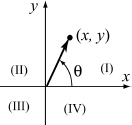
12. Write a user-defined MATLAB function that determines the angle that forms by the intersection of two lines. For the function name and arguments, use th=anglines(A,B,C). The input arguments to the function are vectors with the coordinates of the points A, B, and C, as shown in the figure, which can be two- or three-dimensional. The output th is the angle in degrees. Use the function anglines for determining the angle for the following cases:

(a) A(-5, −1, 6), B(2.5, 1.5, −3.5), C(−2.3, 8, 1)

(b) A(−5.5, 0), B(3.5, −6.5), C(0, 7)

13. Write a user-defined MATLAB function that determines the unit vector in the direction of the line that connects two points (A and B) in space. For the function name and arguments, use n = unitvec(A,B). The input to the function are two vectors A and B, each with the Cartesian coordinates of the corresponding point. The output is a vector with the components of the unit vector in the direction from A to B. If points A and B have two coordinates each (they are in the x y plane), then n is a two-element vector. If points A and B have three coordinate each (general points in space), then n is a three-element vector. Use the function to determine the following unit vectors:

(a) In the direction from point (1.2, 3.5) to point (12, 15)

(b) In the direction from point (−10, −4, 2.5) to point (−13, 6, −5)

14. Write a user-defined MATLAB function that determines the cross product of two vectors. For the function name and arguments, use w=crosspro(u,v). The input arguments to the function are the two vectors, which can be two- or three-dimensional. The output w is the result (a vector). Use the function crosspro for determining the cross product of:

(a) Vectors a = 3i + 11j and b = 14i − 7.3j

(b) Vectors c = −6i + 14.2j + 3k and d = 6.3i − 8j − 5.6k

15. The area of a triangle ABC can be calculated by:

where AB is the vector from point A to point B and AC is the vector from point A to point C. Write a user-defined MATLAB function that determines the area of a triangle given its vertices’ coordinates. For the function name and arguments, use [Area] = TriArea(A,B,C). The input arguments A, B, and C, are vectors, each with the coordinates of the corresponding vertex. Write the code of TriArea such that it has two subfunctions—one that determines the vectors AB and AC and another that executes the cross product. (If available, use the user-defined functions from Problem 14). The function should work for a triangle in the x-y plane (each vertex is defined by two coordinates) or for a triangle in space (each vertex is defined by three coordinates). Use the function to determine the areas of triangles with the following vertices:

(a) A = (1, 2), B = (10, 3), C = (6, 11)

(b) A = (−1.5, −4.2, −3), B = (−5.1, 6.3, 2), C = (12.1, 0, −0.5)

16. Write a user-defined MATLAB function that determines the circumference of a triangle when the coordinates of the vertices are given. For the function name and arguments, use [cr] = cirtriangle(A,B,C). The input arguments A,B,C are vectors with the coordinates of the vertices, and the output variable cr is the circumference. The function should work for a triangle in the x-y plane (each vertex is defined by two coordinates) or for a triangle in space (each vertex is defined by three coordinates). Write the code of cirtriangle such that it has a subfunction or an anonymous function for calculating the distance between two points. Use the function to determine the circumference of triangles with the following vertices:

(a) A = (1, 2), B = (10, 3), C = (6, 11)

(b) A = (−1.5, −4.2, −3), B = (−5.1, 6.3, 2), C = (12.1, 0, −0.5)

17. Write a user-defined function that plots a circle given the coordinates of the center and a point on the circle. For the function name and arguments, use circlePC(c,p). The input argument c is a two-element vector with the x and y coordinates of the center and the input argument p is a two-element vector with the x and y coordinates of the a point on the circle. This function has no output arguments. Use the function to plot the following two circles (both in the same figure):

(a) Center at x = 7.2, y = −2.9, point on the circle at x = −1.8, y = 0.5

(b) Center at x = −0.9, y = −3.3, point on the circle at x = 0, y = 10

18. Write a user-defined MATLAB function that converts integers written in decimal form to binary form. Name the function b=Bina(d), where the input argument d is the integer to be converted and the output argument b is a vector with 1s and 0s that represents the number in binary form. The largest number that could be converted with the function should be a binary number with 16 1s. If a larger number is entered as d, the function should display an error message. Use the function to convert the following numbers:

(a) 100

(b) 1002

(c) 52,601

(c) 200,090

19. Write a user-defined function that plots a triangle and the circle that circumscribes the triangle, given the coordinates of its vertices. For the function name and arguments, use TriCirc(A,B,C). The input arguments are vectors with the x and y coordinates of the vertices, respectively. This function has no output arguments. Use the function with the points (1.5, 3), (9, 10.5), and (6, −3.8).

20. Write a user-defined function that plots an ellipse with axes that are parallel to the x and y axes, given the coordinates of its center and the length of the axes. For the function name and arguments, use ellipseplot(xc,yc,a,b). The input arguments xc and yc are the coordinates of the center, and a and b are half the lengths of the horizontal and vertical axes (see figure), respectively. This function has no output arguments. Use the function to plot the following ellipses:

(a) xc = 3.5, yc = 2.0, a = 8.5, b = 3

(b) xc = −5, yc = 1.5, a = 4, b = 8

21. In polar coordinates a two-dimensional vector is given by its radius and angle (r, θ). Write a user-defined MATLAB function that adds two vectors that are given in polar coordinates. For the function name and arguments, use [r th]= AddVecPol(r1,th1,r2,th2), where the input arguments are (r₁, θ₁) and (r₂, θ₂), and the output arguments are the radius and angle of the result. Use the function to carry out the following additions:

(a) r₁ = (5, 23°), r₂ = (12, 40°)

(b) r₁ = (6, 80°), r₂ = (15, 125°)

22. Write a user-defined function that finds all the prime numbers between two numbers m and n. Name the function pr=prime(m,n), where the input arguments m and n are positive integers and the output argument pr is a vector with the prime numbers. If m > n is entered when the function is called, the error message “The value of n must be larger than the value of m.” is displayed. If a negative number or a number that is not an integer is entered when the function is called, the error message “The input argument must be a positive integer.” is displayed. Do not use MATLAB’s built-in functions primes and isprime. Use the function with:

(a) prime(12,80)

(b) prime(21,63.5)

(c) prime(100,200)

(d) prime(90,50)

23. The geometric mean GM of a set of n positive numbers x₁, x₂, …, x_n is defined by:

GM = (x₁ · x₂ · … · x_n)^1/n

Write a user-defined function that calculates the geometric mean of a set of numbers. For function name and arguments use GM=Geomean(x), where the input argument x is a vector of numbers (any length) and the output argument GM is their geometric mean. The geometric mean is useful for calculating the average of rates. The following table gives the inflation rates in the United States from 1978 to 1987 (inflation of 7.6% means 1.076). Use the user-defined function Geomean to calculate the average inflation for the ten-year period.

24. Write a user-defined function that determines the polar coordinates of a point from the Cartesian coordinates in a two-dimensional plane. For the function name and arguments, use [th rad]=CartToPolar(x,y). The input arguments are the x and y coordinates of the point, and the output arguments are the angle θ and the radial distance to the point. The angle θ is in degrees and is measured relative to the positive x axis, such that it is a positive number in quadrants I and II, and a negative number in quadrant III and IV. Use the function to determine the polar coordinates of points (14, 9), (−11, −20), (−15, 4), and (13.5, −23.5).

25. Write a user-defined function that determines the mode of a set of data (the value in the set that occurs most often). For the function name and arguments, use m=mostfrq(x). The input to the function is a vector x of any length with values, and the output m is a two-element vector in which the first element is the value in x that occurs most often, and the second element is the mode. If there are two, or more, values for the mode the output is the message: “There are more than one value for the mode.” Do not use the MATLAB built-in function mode. Test the function three times. For input create a 20-element vector using the following command: x=randi(10,1,20).

26. Write a user-defined function that sorts the elements of a vector from the largest to the smallest. For the function name and arguments, use y=downsort(x). The input to the function is a vector x of any length, and the output y is a vector in which the elements of x are arranged in a descending order. Do not use the MATLAB built-in functions sort, max, or min. Test your function on a vector with 14 numbers (integers) randomly distributed between −30 and 30. Use the MATLAB randi function to generate the initial vector.

27. Write a user-defined function that sorts the elements of a matrix. For the function name and arguments, use B = matrixsort(A), where A is any size (m × n) matrix and B is a matrix of the same size with the elements of A rearranged in descending order row after row with the (1,1) element the largest and the (m,n) element the smallest. If available, use the user-defined function downsort from Problem 26 as a subfunction within matrixsort.

Test your function on a 4 × 7 matrix with elements (integers) randomly distributed between −30 and 30. Use MATLAB’s randi function to generate the initial matrix.

28. Write a user-defined function that finds the largest element of a matrix. For the function name and arguments, use [Em,rc] = matrixmax(A), where A is any size matrix. The output argument Em is the value of the largest element, and rc is a two-element vector with the address of the largest element (row and column numbers). If there are two, or more, elements that have the maximum value, the output argument rc is a two-column matrix where the rows list the addresses of the elements. Test the function three times. For input create a 4 × 6 matrix using the following command: x=randi([-20 100],4,6)

29. Write a user-defined MATLAB function that calculates the determinant of a 3 × 3 matrix by using the formula:

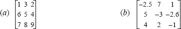
For the function name and arguments, use d3 = det3by3(A), where the input argument A is the matrix and the output argument d3 is the value of the determinant. Write the code of det3by3 such that it has a subfunction that calculates the 2 × 2 determinant. Use det3by3 for calculating the determinants of:

30. A two-dimensional state of stress at a point in a loaded material in the direction defined by the x-y coordinate system is defined by three components of stress σ_xx, σ_yy, and τ_xy. The stresses at the point in the direction defined by the x′-y′ coordinate system are calculated by the stress transformation equations:

where θ is the angle shown in the figure. Write a user-defined MATLAB function that determines the stresses σ_x′x′, σ_y′y′, and τ_x′y′ given the stresses σ_xx, σ_yy, τ_xy, and the angle θ. For the function name and arguments, use [Stran]=StressTrans(S,th). The input argument S is a vector with the values of the three stress components σ_xx, σ_yy, and τ_xy, and the input argument th is a scalar with the value of θ. The output argument Stran is a vector with the values of the three stress components σ_x′x′, σ_y′y′, and τ_x′y′.

Use the function to determine the stresses transformation for the following cases:

(a) σ_xx = 160 MPa, σ_yy = −40 MPa, and τ_xy = 60 MPa, θ = 20°

(b) σ_xx = −18 Ksi, σ_yy = 10 Ksi, and τ_xy = −8 Ksi, θ = 65°

31. The dew point temperature T_d and the relative humidity RH can be calculated (approximately) from the dry-bulb T and wet-bulb T_w temperatures by (http://www.wikipedia.org):

where the temperatures are in degrees Celsius, RH is in %, and p_sta is the barometric pressure in units of millibars.

Write a user-defined MATLAB function that calculates the dew point temperature and relative humidity for given dry-bulb and wet-bulb temperatures in degrees Fahrenheit (°F) and barometric pressure in inches of mercury (inHg). For the function name and arguments, use [Td,RH] = DewptRhum(T,Tw,BP), where the input arguments T,Tw,BP are dry-bulb and wet-bulb temperatures in °F and BP is the barometric pressure in inHg, respectively. The output arguments Td,RH are the dew point temperature in °F and the relative humidity in %. The values of the output arguments should be rounded to the nearest tenth. Use anonymous function or subfunctions inside DewptRhum to convert units.

Use the user-defined function DewptRhum for calculating the dew point temperature and relative humidity for the following cases:

(a) T = 78 °F, T_w = 66 °F, p_sta = 29.09 inHg

(b) T = 97 °F, T_w = 88 °F, p_sta = 30.12 mbar

32. In a lottery the player has to select several numbers out of a list. Write a user-defined function that generates a list of n integers that are uniformly distributed between the numbers a and b. All the selected numbers on the list must be different. For function name and arguments, use x=lotto(a,b,n) where the input argument are the numbers a and b, and n, respectively. The output argument x is a vector with the selected numbers.

(a) Use the function to generate a list of seven numbers from the numbers 1 through 59.

(b) Use the function to generate a list of eight numbers from the numbers 50 through 65.

(c) Use the function to generate a list of nine numbers from the numbers −25 through −2.

33. The Taylor’s series expansion for cosx about x = 0 is given by:

where x is in radians. Write a user-defined function that determines cosx using Taylor’s series expansion. For function name and arguments, use y=cosTay(x), where the input argument x is the angle in degrees and the output argument y is the value for cosx. Inside the user-defined function, use a loop for adding the terms of the Taylor’s series. If a_n is the nth term in the series, then the sum s_n of the n terms is S_n = S_n−1 + a_n. In each pass, calculate the estimated error E given by . Stop adding terms when E ≤ 0.000001. Since cos(θ) = cos (θ ± 360n) write the user-defined function such that if the angle is larger than 360°, or smaller than −360°, then the taylor series will be calculated using the smallest number of terms (using a value for x that is closest to 0).

Use cosTay for calculating:

(a) cos67°

(b) cos200°

(c) cos−80°

(d) cos794°

(e) cos20000°

(f) cos−738°

Compare the values calculated using cosTay with the values obtained by using MATLAB’s built-in cosd function.

34. Write a user-defined function that determines the coordinate y_c of the centroid of the U-shaped cross-sectional area shown in the figure. For the function name and arguments, use yc = centroidU(w,h,t,d), where the input arguments w, h, t, and d, are the dimensions shown in the figure and the output argument yc is the coordinate y_c.

Use the function to determine y_c for an area with w = 10 in., h = 7 in., d = 1.75 in., and t = 0.5 in.

35. The area moment of inertia I_xo of a rectangle about the axis x_o passing through its centroid is . The moment of inertia about an axis x that is parallel to x_o is given by , where A is the area of the rectangle, and d_x is the distance between the two axes.

Write a MATLAB user-defined function that determines the area moment of inertia I_xc of a “U” beam about the axis that passes through its centroid (see drawing). For the function name and arguments use Ixc=IxcT-Beam(w,h,t,d), where the input arguments w, h, t, and d are the dimensions shown in the figure and the output argument Ixc is I_xc. For finding the coordinate y_c of the of the centroid, use the user-defined function centroidU from Problem 34 as a subfunction inside IxcUBeam.
(The moment of inertia of a composite area is obtained by dividing the area into parts and adding the moments of inertia of the parts.)

Use the function to determine the moment of inertia of a “U” beam w = 12 in., h = 8 in., d = 2 in., and t = 0.75 in.

36. In a low-pass RL filter (a filter that passes signals with low frequencies), the ratio of the magnitudes of the voltages is given by:

where ω is the frequency of the input signal.

Write a user-defined MATLAB function that calculates the magnitude ratio. For the function name and arguments, use RV = LRFilt(R,L,w). The input arguments are R, the size of the resistor in Ω (ohms); L, the size of the capacitor in H (Henry); and w, the frequency of the input signal in rad/s. Write the function such that w can be a vector.

Write a program in a script file that uses the LRFilt function to generate a plot of RV as a function of ω for 10 ≤ ω ≤ 10⁶ rad/s. The plot has a logarithmic scale on the horizontal axis (ω). When the script file is executed, it asks the user to enter the values of R and L. Label the axes of the plot.

Run the script file with R = 600 Ω, and L = 0.14 μF.

37. A circuit that filters out a certain frequency is shown in the figure. In this filter, the ratio of the magnitudes of the voltages is given by:

where ω is the frequency of the input signal.

Write a user-defined MATLAB function that calculates the magnitude ratio. For the function name and arguments, use RV=filtfreq(R,C,L,w). The input arguments are R the size of the resistor in Ω (ohms); C, the size of the capacitor in F (farads); L, the inductance of the coil in H (henrys); and w, the frequency of the input signal in rad/s. Write the function such that w can be a vector.

Write a program in a script file that uses the filtfreq function to generate a plot with two graphs of RV as a function of ω for 10 ≤ ω ≤ 10⁴ rad/s. In one graph C = 160 μF, L = 45 mH, and R = 200 Ω, and in the second graph C and L are the same and R = 50 Ω. The plot has a logarithmic scale on the horizontal axis (ω). Label the axes and display a legend.

38. The first derivative of a function f(x) at a point x = x₀ can be approximated with the two-point central difference formula:

where h is a small number relative to x₀. Write a user-defined function function (see Section 7.9) that calculates the derivative of a math function f(y) by using the two-point central difference formula. For the user-defined function name, use dfdx=Funder(Fun,x0), where Fun is a name for the function that is passed into Funder, and x0 is the point where the derivative is calculated. Use h = x₀/100 in the two-point central difference formula. Use the user-defined function Funder to calculate the following:

(a) The derivative of f(x) = x³e^2x at x₀ = 0.6

(b) The derivative of at x₀ = 2.5

In both cases compare the answer obtained from Funder with the analytical solution (use format long).

39. The new coordinates (X_r, Y_r) of a point in the x-y plane that is rotated about the z axis at an angle θ (positive is clockwise) are given by

X_r = X₀cosθ − Y₀sinθ
Y_r = X₀sinθ + Y₀cosθ

where (X₀, Y₀) are the coordinates of the point before the rotation. Write a user-defined function that calculates (X_r, Y_r) given (X₀, Y₀) and θ. For function name and arguments, use [xr,yr]=rotation(x,y,q), where the input arguments are the initial coordinates and the rotation angle in degrees and the output arguments are the new coordinates.

(a) Use rotation to determine the new coordinates of a point originally at (6.5, 2.1) that is rotated about the z-axis by 25°.

(b) Consider the function y = (x − 7)² + 1.5 for 5 ≤ x ≤ 9. Write a program in a script file that makes a plot of the function. Then use rotation to rotate all the points that make up the first plot and make a plot of the rotated function. Make both plots in the same figure and set the range of both axes at 0 to 10.

40. In lottery the player has to guess correctly r numbers that are drawn out of n numbers. The probability, P, of guessing m numbers out of the r numbers can be calculated by the expression:

where . Write a user-defined MATLAB function that calculates P. For the function name and arguments, use P = ProbLottery(m,r,n). The input arguments are m the number of correct guesses; r, the number of numbers that need to be guessed; and n, the number of numbers available. Use a subfunction inside ProbLottery for calculating C_{x, y}.

(a) Use ProbLottery for calculating the probability of correctly selecting 3 of 6 the numbers that are drawn out of 49 numbers in a lottery game.

(b) Consider a lottery game in which 6 numbers are drawn out of 49 numbers. Write a program in a script file that displays a table with seven raws and two columns. The first column has the numbers 0, 1, 2, 3, 4, 5, and 6, which are the number of numbers guessed correctly. The second column show the corresponding probability of making the guess.