Chapter 11

Symbolic Math

All of the mathematical operations done with MATLAB in the first 10 chapters were numerical. The operations were carried out by writing numerical expressions that could contain numbers and variables with preassigned numerical values. When a numerical expression is executed by MATLAB, the outcome is also numerical (a single number or an array with numbers). The number, or numbers, are either exact or a floating point–approximated value. For example, typing 1/4 gives 0.2500—an exact value, and typing 1/3 gives 0.3333—an approximated value.

Many applications in math, science, and engineering require symbolic operations, which are mathematical operations with expressions that contain symbolic variables (variables that don’t have specific numerical values when the operation is executed). The result of such operations is also a mathematical expression in terms of the symbolic variables. One simple example involves solving an algebraic equation that contains several variables and solving for one variable in terms of the others. If a, b, and x are symbolic variables, and ax − b = 0, x can be solved in terms of a and b to give x = b/a. Other examples of symbolic operations are analytical differentiation or integration of mathematical expressions. For instance, the derivative of 2t³ + 5t − 8 with respect to t is 6t² + 5.

MATLAB has the capability of carrying out many types of symbolic operations. The numerical part of the symbolic operation is carried out by MATLAB exactly, with no approximation of numerical values. For example, the result of adding and is and not 0.5833x.

Symbolic operations can be performed by MATLAB once the Symbolic Math Toolbox is installed. The Symbolic Math Toolbox is a collection of MATLAB functions that are used for execution of symbolic operations. The commands and functions for the symbolic operations have the same style and syntax as those for the numerical operations. The symbolic operations themselves are executed primarily by MuPad®, which is mathematical software designed for this purpose. The MuPad software is embedded within MATLAB and is automatically activated when a symbolic MATLAB function is executed. MuPad can also be used as separate independent software. That software uses the MuPAD language, which has a completely different structure and commands than MATLAB. The Symbolic Math Toolbox is included in the student version of MATLAB. In the standard version, the toolbox is purchased separately. To check if the Symbolic Math Toolbox is installed on a computer, the user can type the command ver in the Command Window. In response, MATLAB displays information about the version that is used as well as a list of the toolboxes that are installed.

The starting point for symbolic operations is symbolic objects. Symbolic objects are made of variables and numbers that, when used in mathematical expressions, tell MATLAB to execute the expression symbolically. Typically, the user first defines (creates) the symbolic variables (objects) that are needed, and then uses them to create symbolic expressions that are subsequently used in symbolic operations. If needed, symbolic expressions can be used in numerical operations

The first section in this chapter describes how to define symbolic objects and how to use them to create symbolic expressions. The second section shows how to change the form of existing expressions. Once a symbolic expression has been created, it can be used in mathematical operations. MATLAB has a large selection of functions for this purpose. The next four sections (11.3–11.6) describe how to use MATLAB to solve algebraic equations, to carry out differentiation and integration, and to solve differential equations. Section 11.7 covers plotting symbolic expressions. How to use symbolic expressions in subsequent numerical calculations is explained in the following section.

11.1   SYMBOLIC OBJECTS AND SYMBOLIC EXPRESSIONS

A symbolic object can be a variable (without a preassigned numerical value), a number, or an expression made of symbolic variables and numbers. A symbolic expression is a mathematical expression containing one or more symbolic objects. When typed, a symbolic expression may look like a standard numerical expression. However, because the expression contains symbolic objects, it is executed by MATLAB symbolically.

11.1.1   Creating Symbolic Objects

Symbolic objects can be variables or numbers. They can be created with the sym and/or syms commands. A single symbolic object can be created with the sym command:

where the string, which is the symbolic object, is assigned to a name. The string can be:

   A single letter or a combination of several letters (no spaces). Examples: ‘a’, ‘x’, ‘yad’.

   A combination of letters and digits starting with a letter and with no spaces Examples: ‘xh12’, ‘r2d2’.

   A number. Examples: ‘15’, ‘4’.

In the first two cases (where the string is a single letter, a combination of several letters, or a combination of letters and digits), the symbolic object is a symbolic variable. In this case it is convenient (but not necessary) to give the object the same name as the string. For example, a, bb, and x, can be defined as symbolic variables as follows:

The name of the symbolic object can be different from the name of the variable. For example:

As mentioned, symbolic objects can also be numbers. The numbers don’t have to be typed as strings. For example, the sym command is used next to create symbolic objects from the numbers 5 and 7 and assign them to the variables c and d, respectively.

As shown, when a symbolic object is created and a semicolon is not typed at the end of the command, MATLAB displays the name of the object and the object itself in the next two lines. The display of symbolic objects starts at the beginning of the line and is not indented as is the display of numerical variables. The difference is illustrated below, where a numerical variable is created.

Several symbolic variables can be created in one command by using the syms command, which has the form:

The command creates symbolic objects that have the same names as the symbolic variables. For example, the variables y, z, and d can all be created as symbolic variables in one command by typing:

When the syms command is executed, the variables it creates are not displayed automatically—even if a semicolon is not typed at the end of the command.

11.1.2   Creating Symbolic Expressions

Symbolic expressions are mathematical expressions written in terms of symbolic variables. Once symbolic variables are created, they can be used for creating symbolic expressions. The symbolic expression is a symbolic object (the display is not indented). The form for creating a symbolic expression is:

A few examples are:

When a symbolic expression, which includes mathematical operations that can be executed (addition, subtraction, multiplication, and division), is entered, MATLAB executes the operations as the expression is created. For example:

Notice that all the calculations are carried out exactly, with no numerical approximation. In the last example, and were added by MATLAB to give , and was added to . The operations with the terms that contain only numbers in the symbolic expression are carried out exactly. In the last example, is replaced by .

The difference between exact and approximate calculations is demonstrated in the following example, where the same mathematical operations are carried out—once with symbolic variables and once with numerical variables.

An expression that is created can include both symbolic objects and numerical variables. However, if an expression includes a symbolic object (or several), all the mathematical operations will be carried out exactly. For example, if c is replaced by a in the last expression, the result is exact, as it was in the first example.

Additional facts about symbolic expressions and symbolic objects:

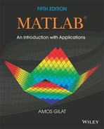
   Symbolic expressions can include numerical variables that have been obtained from the execution of numerical expressions. When these variables are inserted in symbolic expressions their exact value is used, even if the variable was displayed before with an approximated value. For example:

   The double(S) command can be used to convert a symbolic expression (object) S that is written in an exact form to numerical form. (The name “double” comes from the fact that the command returns a double-precision floating-point number representing the value of S.) Two examples are shown. In the first, the p from the last example is converted into numerical form. In the second, a symbolic object is created and then converted into numerical form.

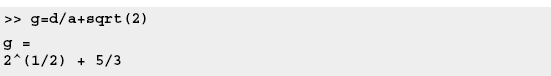
   A symbolic object that is created can also be a symbolic expression written in terms of variables that were not first created as symbolic objects. For example, the quadratic expression ax² + bx + c can be created as a symbolic object named f by using the sym command:

It is important to understand that in this case, the variables a, b, c, and x included in the object do not exist individually as independent symbolic objects (the whole expression is one object). This means that it is impossible to perform symbolic math operations associated with the individual variables in the object. For example, it will not be possible to differentiate f with respect to x. This is different from the way in which the quadratic expression was created in the first example in this section, where the individual variables are first created as symbolic objects and then used in the quadratic expression.

   Existing symbolic expressions can be used to create new symbolic expressions. This is done by simply using the name of the existing expression in the new expression. For example:

11.1.3   The findsym Command and the Default Symbolic Variable

The findsym command can be used to find which symbolic variables are present in an existing symbolic expression. The format of the command is:

The findsym(S)command displays the names of all the symbolic variables (separated by commas) that are in the expression S in alphabetical order. The findsym(S,n) command displays n symbolic variables that are in expression S in the default order. For one-letter symbolic variables, the default order starts with x, and followed by letters, according to their closeness to x. If there are two letters equally close to x, the letter that is after x in alphabetical order is first (y before w, and z before v). The default symbolic variable in a symbolic expression is the first variable in the default order. The default symbolic variable in an expression S can be identified by typing findsym(S,1). Examples:

11.2   CHANGING THE FORM OF AN EXISTING SYMBOLIC EXPRESSION

Symbolic expressions are either created by the user or by MATLAB as the result of symbolic operations. The expressions created by MATLAB might not be in the simplest form or in a form that the user prefers. The form of an existing symbolic expression can be changed by collecting terms with the same power, by expanding products, by factoring out common multipliers, by using mathematical and trigonometric identities, and by many other operations. The following subsections describe several of the commands that can be used to change the form of an existing symbolic expression.

11.2.1   The collect, expand, and factor Commands

The collect, expand, and factor commands can be used to perform the mathematical operations that are implied by their names.

The collect command:

The collect command collects the terms in the expression that have the variable with the same power. In the new expression, the terms will be ordered in decreasing order of power. The command has the forms

where S is the expression. The collect(S) form works best when an expression has only one symbolic variable. If an expression has more than one variable, MATLAB will collect the terms of one variable first, then those of a second variable, and so on. The order of the variables is determined by MATLAB. The user can specify the first variable by using the collect(S, variable_name) form of the command. Examples:

Note that when collect(T) is used, the reformatted expression is written in order of decreasing powers of x, but when collect(T,y) is used, the reformatted expression is written in order of decreasing powers of y.

The expand command:

The expand command expands expressions in two ways. It carries out products of terms that include summation (used with at least one of the terms), and it uses trigonometric identities and exponential and logarithmic laws to expand corresponding terms that include summation. The form of the command is:

where S is the symbolic expression. Two examples are:

The factor command:

The factor command changes an expression that is a polynomial to a product of polynomials of a lower degree. The form of the command is:

where S is the symbolic expression. An example is:

11.2.2   The simplify and simple Commands

The simplify and simple commands are both general tools for simplifying the form of an expression. The simplify command uses built-in simplification rules to generate a simpler form of the expression than the original. The simple command is programmed to generate a form of the expression with the least number of characters. Although there is no guarantee that the form with the least number of characters is the simplest, in actuality this is often the case.

The simplify command:

The simplify command uses mathematical operations (addition, multiplication, rules of fractions, powers, logarithms, etc.) and functional and trigonometric identities to generate a simpler form of the expression. The format of the simplify command is:

Two examples are:

The simple command:

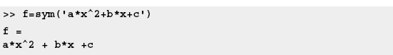
The simple command finds the form of the expression with the fewest number of characters. In many cases this form is also the simplest. When the command is executed, MATLAB creates several forms of the expression by applying the collect, expand, factor, and simplify commands, and other simplification functions that are not covered here. Then MATLAB returns the expression with the shortest form. The simple command has the following three forms:

The difference between the forms is in the output. The use of two of the forms is shown next.

The use of the simple(S) form of the command is not demonstrated because the display of the output is lengthy. MATLAB displays 10 different tries and assigns the shortest form to ans. The reader should try to execute the command and examine the output display.

11.2.3   The pretty Command

The pretty command displays a symbolic expression in a format resembling the mathematical format in which expressions are generally typed. The command has the form

Example:

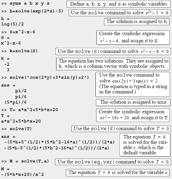
11.3   SOLVING ALGEBRAIC EQUATIONS

A single algebraic equation can be solved for one variable, and a system of equations can be solved for several variables with the solve function.

Solving a single equation:

An algebraic equation can have one or several symbolic variables. If the equation has one variable, the solution is numerical. If the equation has several symbolic variables, a solution can be obtained for any of the variables in terms of the others. The solution is obtained by using the solve command, which has the form

   The argument eq can be the name of a previously created symbolic expression, or an expression that is typed in. When a previously created symbolic expression S is entered for eq, or when an expression that does not contain the = sign is typed in for eq, MATLAB solves the equation eq = 0.

   An equation of the form f(x) = g(x) can be solved by typing the equation (including the = sign) as a string for eq.

   If the equation to be solved has more than one variable, the solve(eq) command solves for the default symbolic variable (see Section 11.1.3). A solution for any of the variables can be obtained with the solve (eq,var) command by typing the variable name for var.

   If the user types solve(eq), the solution is assigned to the variable ans.

   If the equation has more than one solution, the output h is a symbolic column vector with a solution at each element. The elements of the vector are symbolic objects. When an array of symbolic objects is displayed, each row is enclosed with square brackets (see the following examples).

The following examples illustrate the use of the solve command.

   It is also possible to use the solve command by typing the equation to be solved as a string, without having the variables in the equation first created as symbolic objects. However, if the solution contains variables (when the equation has more than one variable), the variables do not exist as independent symbolic objects. For example:

The equation can also be solved for a different variable. For example, a solution for g is obtained by:

Solving a system of equations:

The solve command can also be used for solving a system of equations. If the number of equations and the number of variables are the same, the solution is numerical. If the number of variables is greater than the number of equations, the solution is symbolic for the desired variables in terms of the other variables. A system of equations (depending on the type of equations) can have one or several solutions. If the system has one solution, each of the variables for which the system is solved has one numerical value (or expression). If the system has more than one solution, each of the variables can have several values.

The format of the solve command for solving a system of n equations is:

   The arguments eq1,eq2,...,eqn are the equations to be solved. Each argument can be a name of a previously created symbolic expression, or an expression that is typed in as a string. When a previously created symbolic expression S is entered, the equation is S = 0. When a string that does not contain the = sign is typed in, the equation is expression = 0. An equation that contains the = sign must be typed as a string.

   In the first format, if the number of equations n is equal to the number of variables in the equations, MATLAB gives a numerical solution for all the variables. If the number of variables is greater than the number of equations n, MATLAB gives a solution for n variables in terms of the rest of the variables. The variables for which solutions are obtained are chosen by MATLAB according to the default order (Section 11.1.3).

   When the number of variables is greater than the number of equations n, the user can select the variables for which the system is solved. This is done by using the second format of the solve command and entering the names of the variables var1,var2,...,varn.

The output from the solve command, which is the solution of the system, can have two different forms. One is a cell array and the other is a structure. A cell array is an array in which each of the elements can be an array. A structure is an array in which the elements (called fields) are addressed by textual field designators. The fields of a structure can be arrays of different sizes and types. Cell arrays and structures are not presented in detail in this book, but a short explanation is given below so that the reader will be able to use them with the solve command.

When a cell array is used in the output of the solve command, the command has the following form (in the case of a system of three equations):

[varA, varB, varC] = solve(eq1,eq2,eq3)

   Once the command is executed, the solution is assigned to the variables varA, varB, and varC, and the variables are displayed with their assigned solution. Each of the variables will have one or several values (in a column vector) depending on whether the system of equations has one or several solutions.

   The user can select any names for varA, varB, and varC. MATLAB assigns the solution for the variables in the equations in alphabetical order. For example, if the variables for which the equations are solved are x, u, and t, the solution for t is assigned to varA, the solution for u is assigned to varB, and the solution for x is assigned to varC.

The following examples show how the solve command is used for the case where a cell array is used in the output:

In the example above, notice that the system of two equations is solved by MATLAB for x and y in terms of t, since x and y are the first two variables in the default order. The system, however, can be solved for different variables. As an example, the system is solved next for y and t in terms of x (using the second form of the solve command:

When a structure is used in the output of the solve command, the command has the form (in the case of a system of three equations)

AN = solve(eq1,eq2,eq3)

   AN is the name of the structure.

   Once the command is executed the solution is assigned to AN. MATLAB displays the name of the structure and the names of the fields of the structure, which are the names of the variables for which the equations are solved. The size and the type of each field is displayed next to the field name. The content of each field, which is the solution for the variable, is not displayed.

   To display the content of a field (the solution for the variable), the user has to type the address of the field. The form for typing the address is: structure_name.field_name (see example below).

As an illustration the system of equations solved in the last example is solved again using a structure for the output.

Sample Problem 11-1 shows the solution of a system of equations that has two solutions.

Sample Problem 11-1: Intersection of a circle and a line

The equation of a circle in the x y plane with radius R and its center at point (2, 4) is given by (x − 2)² + (y − 4)² = R². The equation of a line in the plane is given by . Determine the coordinates of the points (as a function of R) where the line intersects the circle.

Solution

The solution is obtained by solving the system of the two equations for x and y in terms of R. To show the difference in the output between using cell array and structure output forms of the solve command, the system is solved twice. The first solution has the output in a cell array:

The second solution has the output in a structure:

11.4   DIFFERENTIATION

Symbolic differentiation can be carried out by using the diff command. The form of the command is:

   Either S can be the name of a previously created symbolic expression, or an expression can be typed in for S.

   In the diff(S) command, if the expression contains one symbolic variable, the differentiation is carried out with respect to that variable. If the expression contains more than one variable, the differentiation is carried out with respect to the default symbolic variable (Section 11.1.3).

   In the diff(S,var) command (which is used for differentiation of expressions with several symbolic variables) the differentiation is carried out with respect to the variable var.

   The second or higher (nth) derivative can be determined with the diff(S,n) or diff(S,var,n) command, where n is a positive number. n = 2 for the second derivative, n = 3 for the third, and so on.

Some examples are:

   It is also possible to use the diff command by typing the expression to be differentiated as a string directly in the command without having the variables in the expression first created as symbolic objects. However, the variables in the differentiated expression do not exist as independent symbolic objects.

11.5   INTEGRATION

Symbolic integration can be carried out by using the int command. The command can be used for determining indefinite integrals (antiderivatives) and definite integrals. For indefinite integration the form of the command is:

   Either S can be the name of a previously created symbolic expression, or an expression can be typed in for S.

   In the int(S) command, if the expression contains one symbolic variable, the integration is carried out with respect to that variable. If the expression contains more than one variable, the integration is carried out with respect to the default symbolic variable (Section 11.1.3).

   In the int(S,var) command, which is used for integration of expressions with several symbolic variables, the integration is carried out with respect to the variable var.

Some examples are:

For definite integration the form of the command is:

   a and b are the limits of integration. The limits can be numbers or symbolic variables.

For example, determination of the definite integral with MATLAB is:

   It is possible also to use the int command by typing the expression to be integrated as a string without having the variables in the expression first created as symbolic objects. However, the variables in the integrated expression do not exist as independent symbolic objects.

   Integration can sometimes be a difficult task. A closed-form answer may not exist, or if it exists, MATLAB might not be able to find it. When that happens MATLAB returns int(S) and the message Explicit integral could not be found.

11.6   SOLVING AN ORDINARY DIFFERENTIAL EQUATION

An ordinary differential equation (ODE) can be solved symbolically with the dsolve command. The command can be used to solve a single equation or a system of equations. Only single equations are addressed here. Chapter 10 discusses using MATLAB to solve first-order ODEs numerically. The reader’s familiarity with the subject of differential equations is assumed. The purpose of this section is to show how to use MATLAB for solving such equations.

A first-order ODE is an equation that contains the derivative of the dependent variable. If t is the independent variable and y is the dependent variable, the equation can be written in the form

A second-order ODE contains the second derivative of the dependent variable (it can also contain the first derivative). Its general form is:

A solution is a function y = f(t) that satisfies the equation. The solution can be general or particular. A general solution contains constants. In a particular solution the constants are determined to have specific numerical values such that the solution satisfies specific initial or boundary conditions.

The command dsolve can be used for obtaining a general solution or, when the initial or boundary conditions are specified, for obtaining a particular solution.

General solution:

For obtaining a general solution, the dsolve command has the form:

   eq is the equation to be solved. It has to be typed as a string (even if the variables are symbolic objects).

   The variables in the equation don’t have to first be created as symbolic objects. (If they have not been created, then, in the solution the variables will not be symbolic objects.)

   Any letter (lowercase or uppercase), except D can be used for the dependent variable.

   In the dsolve(‘eq’) command the independent variable is assumed by MATLAB to be t (default).

   In the dsolve(‘eq’,‘var’) command the user defines the independent variable by typing it for var (as a string).

   In specifying the equation the letter D denotes differentiation. If y is the dependent variable and t is the independent variable, Dy stands for . For example, the equation is typed in as ‘Dy + 3*y = 100’.

   A second derivative is typed as D2, third derivative as D3, and so on. For example, the equation = sin(t) is typed in as: ‘D2y + 3*Dy + 5*y = sin(t)’.

   The variables in the ODE equation that is typed in the dsolve command do not have to be previously created symbolic variables.

   In the solution MATLAB uses C1, C2, C3, and so on, for the constants of integration.

For example, a general solution of the first-order ODE is obtained by:

A general solution of the second-order ODE is obtained by:

The following examples illustrate the solution of differential equations that contain symbolic variables in addition to the independent and dependent variables.

Particular solution:

A particular solution of an ODE can be obtained if boundary (or initial) conditions are specified. A first-order equation requires one condition, a second-order equation requires two conditions, and so on. For obtaining a particular solution, the dsolve command has the form

   For solving equations of higher order, additional boundary conditions have to be entered in the command. If the number of conditions is less than the order of the equation, MATLAB returns a solution that includes constants of integration (C1, C2, C3, and so on).

   The boundary conditions are typed in as strings in the following:

Math form	MATLAB form
y(a)= A	‘y(a)=A’
y’(a)= A	‘Dy (a)=A’
y’’(a)= A	‘D2y(a)=A’

   The argument ‘var’ is optional and is used to define the independent variable in the equation. If none is entered, the default is t.

For example, the first-order ODE , with the initial condition y(0) = 5 is solved with MATLAB by:

The second-order ODE , y(0) = 1, , can be solved with MATLAB by:

Additional examples of solving differential equations are shown in Sample Problem 11-5.

If MATLAB cannot find a solution, it returns an empty symbolic object and the message Warning: explicit solution could not be found.

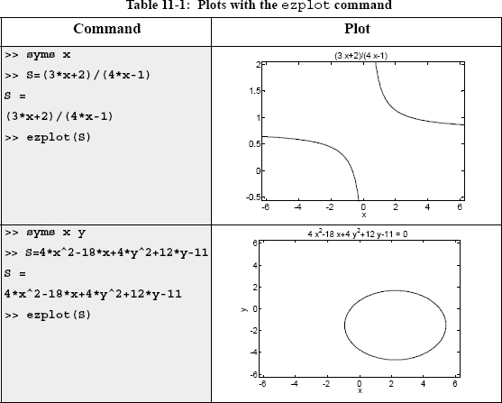
11.7   PLOTTING SYMBOLIC EXPRESSIONS

In many cases, there is a need to plot a symbolic expression. This can easily be done with the ezplot command. For a symbolic expression S that contains one variable var, MATLAB considers the expression to be a function, and the command creates a plot of versus var. For a symbolic expression that contains two symbolic variables var1 and var2, MATLAB considers the expression to be a function in the form, and the command creates a plot of one variable versus the other.

To plot a symbolic expression S that contains one or two variables, the ezplot command is:

•   S is the symbolic expression to be plotted. It can be the name of a previously created symbolic expression, or an expression can be typed in for S.

•   It is also possible to type the expression to be plotted as a string without having the variables in the expression first created as symbolic objects.

•   If S has one symbolic variable, a plot of S(var) versus (var) is created, with the values of var (the independent variable) on the abscissa (horizontal axis), and the values of S(var) on the ordinate (vertical axis).

•   If the symbolic expression S has two symbolic variables, var1 and var2, the expression is assumed to be a function with the form S(var1, var2) = 0. MATLAB creates a plot of one variable versus the other variable. The variable that is first in alphabetic order is taken to be the independent variable. For example, if the variables in S are x and y, then x is the independent variable and is plotted on the abscissa and y is the dependent variable plotted on the ordinate. If the variables in S are u and v, then u is the independent variable and v is the dependent variable.

•   In the ezplot(S) command, if S has one variable (S(var)), the plot is over the domain −2π < var < 2 π (default domain) and the range is selected by MATLAB. If S has two variables (S(var1,var2)), the plot is over −2π < var1 < 2π and −2π < var2 < 2π.

•   In the ezplot(S,[min,max]) command the domain for the independent variable is defined by min and max:—min < var < max—and the range is selected by MATLAB.

•   In the ezplot(S,[xmin,xmax,ymin,ymax]) command the domain for the independent variable is defined by xmin and xmax, and the domain of the dependent variable is defined by ymin and ymax.

The ezplot command can also be used to plot a function that is given in a parametric form. In this case two symbolic expressions, S1 and S2, are involved, where each expression is written in terms of the same symbolic variable (independent parameter). For example, for a plot of y versus x where x = x(t) and y = y(t), the form of the ezplot command is:

•   S1 and S2 are symbolic expressions containing the same single symbolic variable, which is the independent parameter. S1 and S2 can be the names of previously created symbolic expressions, or expressions can be typed in.

•   The command creates a plot of S2(var) versus S1(var). The symbolic expression that is typed first in the command (S1 in the definition above) is used for the horizontal axis, and the expression that is typed second (S2 in the definition above) is used for the vertical axis.

•   In the ezplot(S1,S2)command the domain of the independent variable is 0 < var < 2π (default domain).

•   In the ezplot(S1,S2,[min,max]) command the domain for the independent variable is defined by min and max: min < var < max.

Additional comments:

Once a plot is created, it can be formatted in the same way as plots created with the plot or fplot format. This can be done in two ways: by using commands or by using the Plot Editor (see Section 5.4). When the plot is created, the expression that is plotted is displayed automatically at the top of the plot. MATLAB has additional plot functions for plotting two-dimensional polar plots and for plotting three-dimensional plots. For more information, the reader is referred to the Help menu of the Symbolic Math Toolbox.

Several examples of using the ezplot command are shown in Table 11-1.

11.8 NUMERICAL CALCULATIONS WITH SYMBOLIC EXPRESSIONS

Once a symbolic expression is created by the user or by the output from any of MATLAB’s symbolic operations, there may be a need to substitute numbers for the symbolic variables and calculate the numerical value of the expression. This can be done by using the subs command. The subs command has several forms and can be used in different ways. The following describes several forms that are easy to use and are suitable for most applications. In one form, the variable (or variables) for which a numerical value is substituted and the numerical value itself are typed inside the subs command. In another form, each variable is assigned a numerical value in a separate command and then the variable is substituted in the expression.

The subs command in which the variable and its value are typed inside the command is shown first. Two cases are presented—one for substituting a numerical value (or values) for one symbolic variable, and the other for substituting numerical values for two or more symbolic variables.

Substituting a numerical value for one symbolic variable:

A numerical value (or values) can be substituted for one symbolic variable when a symbolic expression has one or more symbolic variables. In this case the subs command has the form:

•   number can be one number (a scalar), or an array with many elements (a vector or a matrix).

•   The value of S is calculated for each value of number and the result is assigned to R, which will have the same size as number (scalar, vector, or matrix).

•   If S has one variable, the output R is numerical. If S has several variables and a numerical value is substituted for only one of them, the output R is a symbolic expression.

An example with an expression that includes one symbolic variable is:

In the last example, notice that when the numerical value of the symbolic expression is calculated, the answer is numerical (the display is indented). An example of substituting numerical values for one symbolic variable in an expression that has several symbolic variables is:

Substituting a numerical value for two or more symbolic variables:

A numerical value (or values) can be substituted for two or more symbolic variables when a symbolic expression has several symbolic variables. In this case the subs command has the following form (it is shown for two variables, but it can be used in the same form for more):

•   The variables var1 and var2 are the variables in the expression S for which the numerical values are substituted. The variables are typed as a cell array (inside curly braces {}). A cell array is an array of cells where each cell can be an array of numbers or text.

•   The numbers number1,number2 substituted for the variables are also typed as a cell array (inside curly braces {}). The numbers can be scalars, vectors, or matrices. The first cell in the numbers cell array (number1) is substituted for the variable that is in the first cell of the variable cell array (var1), and so on.

•   If all the numbers that are substituted for variables are scalars, the outcome will be one number or one expression (if some of the variables are still symbolic).

•   If, for at least one variable, the substituted numbers are an array, the mathematical operations are executed element-by-element and the outcome is an array of numbers or expressions. It should be emphasized that the calculations are performed element-by-element even though the expression S is not typed in the element-by-element notation. This also means that all the arrays substituted for different variables must be of the same size.

•   It is possible to substitute arrays (of the same size) for some of the variables and scalars for other variables. In this case, in order to carry out element-by-element operations, MATLAB expands the scalars (array of 1s times the scalar) to produce an array result.

The substitution of numerical values for two or more variables is demonstrated in the next examples.

A second method for substituting numerical values for symbolic variables in a symbolic expression is to first assign numerical values to the variables and then use the subs command. In this method, once the symbolic expression exists (at which point the variables in the expression are symbolic) the variables are assigned numerical values. Then the subs command is used in the form:

Once the symbolic variables are redefined as numerical variables they can no longer be used as symbolic. The method is demonstrated in the following examples.

11.9 EXAMPLES OF MATLAB APPLICATIONS

Sample Problem 11-2: Firing angle of a projectile

A projectile is fired at a speed of 210 m/s and an angle θ. The projectile’s intended target is 2,600 m away and 350 m above the firing point.

(a) Derive the equation that has to be solved in order to determine the angle θ? such that the projectile will hit the target.

(b) Use MATLAB to solve the equation derived in part (a).

(c) For the angle determined in part (b), use the ezplot command to make a plot of the projectile’s trajectory.

Solution

(a) The motion of the projectile can be analyzed by considering the horizontal and vertical components. The initial velocity v₀ can be resolved into horizontal and vertical components:

v_0x = v₀ cos(θ) and v_0y = v₀ sin(θ)

In the horizontal direction the velocity is constant, and the position of the projectile as a function of time is given by:

x = v_0x^t

Substituting x = 2600 m for the horizontal distance that the projectile travels to reach the target and 210 cos(θ) for v_0x, and solving for t gives:

In the vertical direction the position of the projectile is given by:

Substituting y = 350 m for the vertical coordinate of the target, 210 sin (θ) for v_0x g = 9.81, and t gives:

The solution of this equation gives the angle θ at which the projectile has to be fired.

(b) A solution of the equation derived in part (a) obtained by using the solve command (in the Command Window) is:

(c) The solution from part (b) shows that there are two possible angles and thus two trajectories. In order to make a plot of a trajectory, the x and y coordinates of the projectile are written in terms of t (parametric form):

The domain for t is t = 0 to .

These equations can be used in the ezplot command to make the plots shown in the following program written in a script file.

When this program is executed, the following plot is generated in the Figure Window:

Sample Problem 11-3: Bending resistance of a beam

The bending resistance of a rectangular beam of width b and height h is proportional to the beam’s moment of inertia I, defined by . A rectangular beam is cut out of a cylindrical log of radius R. Determine b and h (as a function of R) such that the beam will have maximum I.

Solution

The problem is solved by following these steps:

1. Write an equation that relates R, h, and b.

2. Derive an expression for I in terms of h.

3. Take the derivative of I with respect to h.

4. Set the derivative equal to zero and solve for h.

5. Determine the corresponding b.

The first step is carried out by looking at the triangle in the figure. The relationship between R, h, and b is given by the Pythagorean theorem as . Solving this equation for b gives .

The rest of the steps are done using MATLAB:

Sample Problem 11-4: Fuel level in a tank

The horizontal cylindrical tank shown is used to store fuel. The tank has a diameter of 6 m and is 8 m long. The amount of fuel in the tank can be estimated by looking at the level of the fuel through a narrow vertical glass window at the front of the tank. A scale that is marked next to the window shows the levels of the fuel corresponding to 40, 60, 80, 120, and 160 thousand liters. Determine the vertical positions (measured from the ground) of the lines of the scale.

Solution

The relationship between the level of the fuel and its volume can be written in the form of a definite integral. Once the integration is carried out, an equation is obtained for the volume in terms of the fuel’s height. The height corresponding to a specific volume can then be determined from solving the equation for the height.

The volume of the fuel V can be determined by multiplying the area of the cross section of the fuel A (the shaded area) by the length of the tank L. The cross-sectional area can be calculated by integration.

The width w of the top surface of the fuel can be written as a function of y. From the triangle in the figure on the right, the variables y, w, and R are related by:

Solving this equation for w gives:

The volume of the fuel at height h can now be calculated by substituting w in the integral in the equation for the volume and carrying out the integration. The result is an equation that gives the volume V as a function of h. The value of h for a given V is obtained by solving the equation for h. In the present problem values of h have to be determined for volumes of 40, 60, 80, 120, and 160 thousand liters. The solution is given in the following MATLAB program (script file):

When the script file is executed, the outcomes from commands that don’t have a semicolon at the end are displayed. The display in the Command Window is:

Units: The unit for length in the solution is meters, which correspond to m³ for the volume (1 m³ = 1,000 L).

Sample Problem 11-5: Amount of medication in the body

The amount M of medication present in the body depends on the rate at which the medication is consumed by the body and on the rate at which the medication enters the body, where the rate at which the medication is consumed is proportional to the amount present in the body. A differential equation for M is

where k is the proportionality constant and p is the rate at which the medication is injected into the body.

(a) Determine k if the half-life of the medication is 3 hours.

(b) A patient is admitted to a hospital and the medication is given at a rate of 50 mg per hour. (Initially there is no medication in the patient’s body.) Derive an expression for M as a function of time.

(c) Plot M as a function of time for the first 24 hours.

Solution

(a) The proportionality constant can be determined from considering the case in which the medication is consumed by the body and no new medication is given. In this case the differential equation is:

The equation can be solved with the initial condition M = M₀ at t = 0:

The solution gives M as a function of time:

A half-life of 3 hours means that at t = 3 hours Substituting this information in the solution gives , and the constant k is determined from solving this equation:

(b) For this part the differential equation for M is:

The constant k is known from part (a), and p = 50 mg/h is given. The initial condition is that in the beginning there is no medication in the patient’s body, or M = 0 at t = 0. The solution of this equation with MATLAB is:

(c) A plot of Mtb as a function of time for 0 < ≤ t ≤ 24 can be done by using the ezplot command:

In the actual display of the last expression that was generated by MATLAB (Mtt = . . .) the numbers have many more decimal digits than shown above. The numbers were shortened so that they will fit on the page.

The plot that is generated is:

11.10 PROBLEMS

1. Define x as a symbolic variable and create the two symbolic expressions

S₁ = x²(x − 6)+ 4(3x − 2) and S₂ = (x + 2)² − 8x

Use symbolic operations to determine the simplest form of each of following expressions:

(a) S₁ · S₂

(b)

(c) S₁ + S₂

(d) Use the subs command to evaluate the numerical value of the result from part (c) for x = 5.

2. Define y as a symbolic variable and create the two symbolic expressions

S₁ = x(x² + 6x + 12) + 8 and S₂ = (x − 3)² + 10x − 5

Use symbolic operations to determine the simplest form of each of following expressions:

(a) S₁ · S₂

(b)

(c) S₁ + S₂

(d) Use the subs command to evaluate the numerical value of the result from part (c) for x = 3.

3. Define x and y as symbolic variables and create the two symbolic expressions

Use symbolic operations to determine the simplest form of S · T. Use the subs command to evaluate the numerical value of the result for x = 9 and y = 2.

4. Define x as a symbolic variable.

(a) Derive the equation of the polynomial that has the roots x = −2, x = −0.5, x = 2, and x = 4.5.

(b) Determine the roots of the polynomial

f(x) = x⁶ − 6.5x⁵ − 58x⁴ + 167.5x³ + 728x² − 890x − 1400

by using the factor command.

5. Use the commands from Section 11.2 to show that:

(a) sin(4x) = 4sinxcosx − 8sin³x cosx

(b)

6. Use the commands from Section 11.2 to show that:

7. The folium of Descartes is the graph shown in the figure. In parametric form its equation is given by:

(a) Use MATLAB to show that the equation of the folium of Descartes can also be written as:

x³ + y³ = 3xy

(b) Make a plot of the folium for the domain shown in the figure by using the ezplot command.

8. A water tower has the geometry shown in the figure (the lower part is a cylinder with radius R and height h, and the upper part is a half sphere with radius R). Determine the radius R if h = 10m and the volume is 1,050 m³. (Write an equation for the volume in terms of the radius and the height. Solve the equation for the radius, and use the double command to obtain a numerical value.

9. The relation between the tension T and the steady shortening velocity v in a muscle is given by the Hill equation:

(T + a)(v + b) = (T₀ + a)b

where a and b are positive constants and T₀ is the isometric tension, i.e., the tension in the muscle when v = 0. The maximum shortening velocity occurs when T = 0.

(a) Using symbolic operations, create the Hill equation as a symbolic expression. Then use subs to substitute T = 0, and finally solve for v to show that v_max = (bT₀)/a.

(b) Use v_max from part (a) to eliminate the constant b from the Hill equation, and show that .

10. Consider the two ellipses in the x y plane given by the equations

(a) Use the ezplot command to plot the two ellipses in the same figure.

(b) Determine the coordinates of the points where the ellipses intersect.

11. A 120 in.–long beam AB is attached to the wall with a pin at point A and to a 66 in.–long cable CD. A load W = 200 lb is attached to the beam at point B. The tension in the cable T and the x and y components of the force at A (F_Ax and F_Ay) can be calculated from the equations:

where L and L_c are the lengths of the beam and the cable, respectively, and d is the distance from point A to point D where the cable is attached.

(a) Use MATLAB to solve the equations for the forces T, F_Ax, and F_Ay in terms of d, L, L_C, and W. Determine F_A given by .

(b) Use the subs command to substitute W = 200 lb, L = 120 in., and L_c = 66 in. into the expressions derived in part (a). This will give the forces as a function of the distance d.

(c) Use the ezplot command to plot the forces T and F_A (both in the same figure as functions of d, for d starting at 20 and ending at 70 in.

(d) Determine the distance d where the tension in the cable is the smallest. Determine the value of this force.

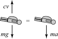
12. A box of mass m is being pulled by a rope as shown. The force F in the rope as a function of x can be calculated from the equations:

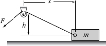
where N and μ are the normal force and friction coefficient between the box and surface, respectively. Consider the case where m = 18kg, h = 10 m, μ = 0.55, and g = 9.81 m/s².

(a) Use MATLAB to derive an expression for F, in terms of x, h, m, g, and μ.

(b) Use the subs command to substitute m = 18kg, h = 10 m, μ = 0.55, and g = 9.81 m/s² into the expressions that were derived in part (a). This will give the force as a function of the distance x.

(c) Use the ezplot command to plot the force F as a function of x, for x starting at 5 and ending at 30 m.

(d) Determine the distance x where the force that is required to pull the box is the smallest, and determine the magnitude of that force.

13. The mechanical power output P in a contracting muscle is given by:

where T is the muscle tension, v is the shortening velocity (max of v_max), T₀ is the isometric tension (i.e., tension at zero velocity), and k is a non-dimensional constant that ranges between 0.15 and 0.25 for most muscles. The equation can be written in non-dimensional form:

where p = (Tv)/(T_0^vmax), and u = v/v_max. Consider the case k = 0.25.

(a) Plot p versus u for 0 ≤ u ≤ 1.

(b) Use differentiation to find the value of u where p is maximum.

(c) Find the maximum value of p.

14. The equation of a circle is x² + y² = R², where R is the radius of the circle. Write a program in a script file that first derives the equation (symbolically) of the tangent line to the circle at the point (x₀, y₀) on the upper part of the circle (i.e., for −R < x₀ < R and 0 < y₀). Then for specific values of −R < x₀, and y₀ the program makes a plot, like the one shown on the right, of the circle and the tangent line. Execute the program with R = 10 and x₀ = 7.

15. A tracking radar antenna is locked on an airplane flying at a constant altitude of 5 km, and a constant speed of 540 km/h. The airplane travels along a path that passes exactly above the radar station. The radar starts the tracking when the airplane is 100 km away.

(a) Derive an expression for the angle θ of the radar antenna as a function of time.

(b) Derive an expression for the angular velocity of the antenna, , as a function of time.

(c) Make two plots on the same page, one of θ versus time and the other of versus time, where the angle is in degrees and the time is in minutes for 0 ≤ t ≤ 20 min.

16. Evaluate the following indefinite integrals:

17. Define x as a symbolic variable and create the symbolic expression

Plot S in the domain 0 ≤ x ≤ π and calculate the integral .

18. The parametric equations of an ellipsoid are:

x = a cosusinv, y = b sinusinv, z = c cosv

where 0 ≤ u ≤ 2π and −π ≤ v ≤ 0

Show that the differential volume element of the ellipsoid shown is given by:

dV = −πabcsin³vdv

Use MATLAB to evaluate the integral of dV from −π to 0 symbolically and show that the volume of the ellipsoid is .

19. The one-dimensional diffusion equation is given by:

Show that the following are solutions to the diffusion equation.

(a) , where A and B are constants.

(b) u = Aexp(−αx)cos(αx − 2mα²t + B)+C where A, B, C, and α, are constants.

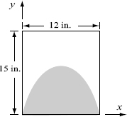
20. A ceramic tile has the design shown in the figure. The shaded area is painted red and the rest of the tile is white. The border line between the red and the white areas follows the equation

y = −kx² + 12kx

Determine k such that the areas of the white and the red colors will be the same.

21. Show that the location of the centroid y_c of the half-circle area shown is given by . The coordinate y_c can be calculated by:

22. For the half-circle area shown in the previous problem, show that the moment of inertia about the x axis, I_x, is given by . The moment of inertia I_x can be calculated by:

23. The rms value of an AC voltage is defined by

where T is the period of the waveform.

(a) A voltage is given by v(t) = Vcos(ωt). Show that and is independent of ω. (The relationship between the period T and the radian frequency ω is .)

(b) A voltage is given by v(t) = 2.5 cos(350t)+ 3 V. Determine v_rms.

24. The spread of an infection from a single individual to a population of N uninfected persons can be described by the equation

with initial condition x(0) = N

where x is the number of uninfected individuals and R is a positive rate constant. Solve this differential equation symbolically for x(t). Also, determine symbolically the time t at which the infection rate dx/dt is maximum.

25. The Maxwell-Boltzmann probability density function f(v) is given by

where m (kg) is the mass of each molecule, v (m/s) is the speed, T (K) is the temperature, and k = 1.38 × 10⁻²³ J/K is Boltzmann’s constant. The most probable speed v_p corresponds to the maximum value of f(v) and can be determined from . Create a symbolic expression for f(v), differentiate it with respect to v and show that . Calculate v_p for oxygen molecules . Make a plot of f(v) versus v for 0 ≤ v ≤ 2500 m/s for oxygen molecules

26. The velocity of a skydiver whose parachute is still closed can be modeled by assuming that the air resistance is proportional to the velocity. From Newton’s second law of motion the relationship between the mass m of the skydiver and his velocity v is given by (down is positive)

where c is a drag constant and g is the gravitational constant (g = 9.81 m/s²).

(a) Solve the equation for v in terms of m, g, c, and t, assuming that the initial velocity of the skydiver is zero.

(b) It is observed that 4 s after a 90 kg skydiver jumps out of an airplane, his velocity is 28 m/s. Determine the constant c.

(c) Make a plot of the skydiver velocity as a function of time for 0 ≤ t ≤ 30s.

27. A resistor R (R = 0.4Ω) and an inductor L (L = 0.08H) are connected as shown. Initially, the switch is connected to point A and there is no current in the circuit. At t = 0 the switch is moved from A to B, so that the resistor and the inductor are connected to v (v_s = 6 V), and current starts flowing in the circuit. The switch remains connected to B until the voltage on the resistor reaches 5 V. At that time (t_BA) the switch is moved back to A.

The current i in the circuit can be calculated from solving the differential equations:

The voltage across the resistor,v_R, at any time is given by v_R = iR.

(a)  Derive an expression for the current i in terms of R, L, v_s, and t for 0 ≤ t ≤ t_BA by solving the first differential equation.

(b)  Substitute the values of R, L, and v_S in the solution for i, and determine the time t_BA when the voltage across the resistor reaches 5 V.

(c)  Derive an expression for the current i in terms of R, L, and t, for t_BA ≤t by solving the second differential equation.

(d)  Make two plots (on the same page), one for v_R versus t for 0 ≤ t ≤ t_BA and the other for v_R versus t for t_BA ≤ t ≤ 2t_BA.

28. Determine the general solution of the differential equation

Show that the solution is correct. (Derive the first derivative of the solution, and then substitute back into the equation.)

29. Determine the solution of the following differential equation that satisfies the given initial conditions. Plot the solution for 0 ≤ t ≤ 7.

30. The current, i, in a series RLC circuit when the switch is closed at t = 0 can be determined from the solution of the 2nd-order ODE

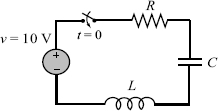
where R, L, and C are the resistance of the resistor, the inductance of the inductor, and the capacitance of the capacitor, respectively.

(a) Solve the equation for i in terms of L, R, C, and t, assuming that at t = 0 t = 0 and di/dt = 8.

(b) Use the subs command to substitute L = 3 H, R = 10Ω, and C = 80 μF into the expression that were derived in part (a). Make a plot of i versus t for 0 ≤ t ≤ 1. (Underdamped response.)

(c) Use the subs command to substitute L = 3 H, R = 200Ω, and C = 1200 μF into the expression that were derived in part (a). Make a plot of i versus t for 0 ≤ t ≤ 2.s. (Overdamped response.)

(d) Use the subs command to substitute L = 3 H, R = 201 Ω, and C = 300 μF into the expression that were derived in part (a). Make a plot of i versus t for 0 ≤ t ≤ 2 s. (Critically damped response.)

31. Damped free vibrations can be modeled by a block of mass m that is attached to a spring and a dash-pot as shown. From Newton’s second law of motion, the displacement x of the mass as a function of time can be determined by solving the differential equation

where k is the spring constant and c is the damping coefficient of the dashpot. If the mass is displaced from its equilibrium position and then released, it will start oscillating back and forth. The nature of the oscillations depends on the size of the mass and the values of k and c.

For the system shown in the figure, m = 10kg and N/m. At time t = 0 the mass is displaced to x =0.18m and then released from rest. Derive expressions for the displacement x and the velocity v of the mass, as a function of time. Consider the following two cases:

(a) c = 3 (N s)/m.

(b) c = 50(N s)/m.

For each case, plot the position x and the velocity v versus time (two plots on one page). For case (a) take 0 ≤ t ≤ 20 s, and for case (b) take 0 ≤ t ≤ 10 s.