Chapter 9

Applications in Numerical Analysis

Numerical methods are commonly used for solving mathematical problems that are formulated in science and engineering where it is difficult or impossible to obtain exact solutions. MATLAB has a large library of functions for numerically solving a wide variety of mathematical problems. This chapter explains a number of the most frequently used of these functions. It should be pointed out here that the purpose of this book is to show users how to use MATLAB. Some general information on the numerical methods is given, but the details, which can be found in books on numerical analysis, are not included.

The following topics are presented in this chapter: solving an equation with one unknown, finding a minimum or a maximum of a function, numerical integration, and solving a first-order ordinary differential equation.

9.1  SOLVING AN EQUATION WITH ONE VARIABLE

An equation with one variable can be written in the form f(x) = 0. A solution to the equation (also called a root) is a numerical value of x that satisfies the equation. Graphically, a solution is a point where the function f(x) crosses or touches the x axis. An exact solution is a value of x for which the value of the function is exactly zero. If such a value does not exist or is difficult to determine, a numerical solution can be determined by finding an x that is very close to the solution. This is done by the iterative process, where in each iteration the computer determines a value of x that is closer to the solution. The iterations stop when the difference in x between two iterations is smaller than some measure. In general, a function can have zero, one, several, or an infinite number of solutions.

In MATLAB a zero of a function can be determined with the command (built-in function) fzero with the form:

The built-in function fzero is a MATLAB function function (see Section 7.9), which means that it accepts another function (the function to be solved) as an input argument.

Additional details on the arguments of fzero:

•  x is the solution, which is a scalar.

•  function is the function to be solved. It can be entered in several different ways:

1.  The simplest way is to enter the mathematical expression as a string.

2.  The function is created as a user-defined function in a function file and then the function handle is entered (see Section 7.9.1).

3.  The function is created as an anonymous function (see Section 7.8.1) and then the name of the anonymous function (which is the name of the handle) is entered (see Section 7.9.1).

(As explained in Section 7.9.2, it is also possible to pass a user-defined function and an inline function into a function function by using its name. However, function handles are more efficient and easier to use, and should be the preferred method.)

•  The function has to be written in a standard form. For example, if the function to be solved is xe^−x = 0.2, it has to be written as f(x) = xe^−x − 0.2 = 0. If this function is entered into the fzero command as a string, it is typed as: ‘x*exp(-x)-0.2’.

•  When a function is entered as an expression (string), it cannot include predefined variables. For example, if the function to be entered is f(x) = xe^−x −0.2, it is not possible to define b=0.2 and then enter ‘x*exp(-x)-b’.

•  x0 can be a scalar or a two-element vector. If it is entered as a scalar, it has to be a value of x near the point where the function crosses (or touches) the x axis. If x0 is entered as a vector, the two elements have to be points on opposite sides of the solution. If f(x) crosses the x axis, then has a f(x0(1)) different sign than f(x0(2)). When a function has more than one solution, each solution can be determined separately by using the fzero function and entering values for x0 that are near each of the solutions.

•  A good way to find approximately where a function has a solution is to make a plot of the function. In many applications in science and engineering the domain of the solution can be estimated. Often when a function has more than one solution only one of the solutions will have a physical meaning.

Sample Problem 9-1: Solving a nonlinear equation

Determine the solution of the equation xe^−x = 0.2.

Solution

The equation is first written in the form of a function: f(x) = xe^−x −0.2. A plot of the function, shown on the right, shows that the function has one solution between 0 and 1 and another solution between 2 and 3. The plot is obtained by typing

in the Command Window. The solutions of the function are found by using the fzero command twice. First the equation is entered as a string expression, and a value of x0 between 0 and 1 (x0 = 0.7) is used. Second, the equation to be solved is written as an anonymous function, which is then used in fzero with x0 between 2 and 3 (x0 = 2.8). This is shown below:

Additional comments:

•  The fzero command finds zeros of a function only where the function crosses the x axis. The command does not find a zero at points where the function touches but does not cross the x axis.

•  If a solution cannot be determined, NaN is assigned to x.

•  The fzero command has additional options (see the Help Window). Two of the more important options are:
[x fval]=fzero(function, x0) assigns the value of the function at x to the variable fval.
x=fzero(function, x0, optimset(‘display’,‘iter’)) displays the output of each iteration during the process of finding the solution.

•  When the function can be written in the form of a polynomial, the solution, or the roots, can be found with the roots command, as explained in Chapter 8 (Section 8.1.2).

•  The fzero command can also be used to find the value of x where the function has a specific value. This is done by translating the function up or down. For example, in the function of Sample Problem 9-1 the first value of x where the function is equal to 0.1 can be determined by solving the equation xe^−x −0.3 = 0. This is shown below:

9.2 FINDING A MINIMUM OR A MAXIMUM OF A FUNCTION

In many applications there is a need to determine the local minimum or maximum of a function of the form y = f(x). In calculus the value of x that corresponds to a local minimum or maximum is determined by finding the zero of the derivative of the function. The value of y is determined by substituting the x into the function. In MATLAB the value of x where a one-variable function f(x) within the interval x₁ ≤ x ≤ x₂ has a minimum can be determined with the fminbnd command which has the form:

•  The function can be entered as a string expression, or as a function handle, in the same way as with the fzero command. See Section 9.1 for details.

•  The value of the function at the minimum can be added to the output by using the option

[x fval]=fminbnd(function,x1,x2)

where the value of the function at x is assigned to the variable fval.

•  Within a given interval, the minimum of a function can either be at one of the end points of the interval or at a point within the interval where the slope of the function is zero (local minimum). When the fminbnd command is executed, MATLAB looks for a local minimum. If a local minimum is found, its value is compared to the value of the function at the end points of the interval. MATLAB returns the point with the actual minimum value for the interval.

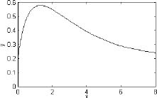
For example, consider the function f(x) = x³ − 12x² + 40.25x − 36.5, which is plotted in the interval 0 ≤ x ≤ 8 in the figure on the right. It can be observed that there is a local minimum between 5 and 6, and that the absolute minimum is at x = 0. Using the fminbnd command with the interval 3 ≤ x ≤ 8 to find the location of the local minimum and the value of the function at this point gives:

Notice that the fminbnd command gives the local minimum. If the interval is changed to 0 ≤ x ≤ 8, fminbnd gives:

For this interval the fminbnd command gives the absolute minimum which is at the end point x = 0.

•  The fminbnd command can also be used to find the maximum of a function. This is done by multiplying the function by −1 and finding the minimum. For example, the maximum of the function f(x) = xe^−x −0.2 (from Sample Problem 9-1) in the interval 0 ≤ x ≤ 8 can be determined by finding the minimum of the function f(x) = − xe^−x + 0.2 as shown below:

9.3 NUMERICAL INTEGRATION

Integration is a common mathematical operation in science and engineering. Calculating area and volume, velocity from acceleration, and work from force and displacement are just a few examples where integrals are used. Integration of simple functions can be done analytically, but more involved functions are frequently difficult or impossible to integrate analytically. In calculus courses the integrand (the quantity to be integrated) is usually a function. In applications of science and engineering the integrand can be a function or a set of data points. For example, data points from discrete measurements of flow velocity can be used to calculate volume.

It is assumed in the presentation below that the reader has knowledge of integrals and integration. A definite integral of a function f(x) from a to b has the form:

The function f(x) is called the integrand, and the numbers a and b are the limits of integration. Graphically, the value of the integral q is the area between the graph of the function, the x axis, and the limits a and b (the shaded area in the figure). When a definite integral is calculated analytically f(x) is always a function. When the integral is calculated numerically f(x) can be a function or a set of points. In numerical integration the total area is obtained by dividing the area into small sections, calculating the area of each section, and adding them up. Various numerical methods have been developed for this purpose. The difference between the methods is in the way that the area is divided into sections and the method by which the area of each section is calculated. Books on numerical analysis include details of the numerical techniques.

The following discussion describes how to use the three MATLAB built-in integration functions quad, quadl, and trapz. The quad and quadl commands are used for integration when f(x) is a function, and trapz is used when f(x) is given by data points.

The quad command:

The form of the quad command, which uses the adaptive Simpson method of integration, is:

•  The function can be entered as a string expression or as a function handle, in the same way as with the fzero command. See Section 9.1 for details. The first two methods are demonstrated in Sample Problem 9-2.

•  The function f(x) must be written for an argument x that is a vector (use element-by-element operations) such that it calculates the value of the function for each element of x.

•  The user has to make sure that the function does not have a vertical asymptote between a and b.

•  quad calculates the integral with an absolute error that is smaller than 1.0e–6. This number can be changed by adding an optional tol argument to the command:

q = quad(‘function’,a,b,tol)

tol is a number that defines the maximum error. With larger tol the integral is calculated less accurately but faster.

The quadl command:

The form of the quadl (the last letter is a lowercase L) command is exactly the same as that of the quad command:

All of the comments that are listed for the quad command are valid for the quadl command. The difference between the two commands is the numerical method used for calculating the integration. The quadl command uses the adaptive Lobatto method, which can be more efficient for high accuracies and smooth integrals.

Sample Problem 9-2: Numerical integration of a function

Use numerical integration to calculate the following integral:

Solution

For illustration, a plot of the function for the interval 0 ≤ x ≤ 8 is shown on the right. The solution uses the quad command and shows how to enter the function in the command in two ways. In the first, it is entered directly by typing the expression as an argument. In the second, an anonymous function is created and its name is subsequently entered in the command.

The use of the quad command in the Command Window, with the function to be integrated typed in as a string, is shown below. Note that the function is typed with element-by-element operations.

The second method is to first create a user-defined function that calculates the function to be integrated. The function file (named y=Chap9Sam2(x)) is:

Note again that the function is written with element-by-element operations such that the argument x can be a vector. The integration is then done in the Command Window by typing the handle @Chap9Sam2 for the argument function in the quad command as shown below:

The trapz command:

The trapz command can be used for integrating a function that is given as data points. It uses the numerical trapezoidal method of integration. The form of the command is

where x and y are vectors with the x and y coordinates of the points, respectively. The two vectors must be of the same length.

9.4 ORDINARY DIFFERENTIAL EQUATIONS

Differential equations play a crucial role in science and engineering since they are in the foundation of virtually every physical phenomenon that is involved in engineering applications. Only a limited number of differential equations can be solved analytically. Numerical methods, on the other hand, can result in an approximate solution to almost any equation. Obtaining a numerical solution might not be simple task however. This is because a numerical method that can solve any equation does not exist. Instead, there are many methods that are suitable for solving different types of equations. MATLAB has a large library of tools that can be used for solving differential equations. To fully utilize the power of MATLAB, however, requires that the user have knowledge of differential equations and the various numerical methods that can be used for solving them.

This section describes in detail how to use MATLAB to solve a first-order ordinary differential equation. The possible numerical methods that can be used for solving such an equation are described in general terms, but are not explained from a mathematical point of view. This section provides information for solving simple, “nonproblematic” first-order equations. This solution provides the basis for solving higher-order equations and systems of equations.

An ordinary differential equation (ODE) is an equation that contains an independent variable, a dependent variable, and derivatives of the dependent variable. The equations that are considered here are of first order with the form

where x and y are the independent and dependent variables, respectively. A solution is a function y = f(x) that satisfies the equation. In general, many functions can satisfy a given ODE, and more information is required for determining the solution of a specific problem. The additional information is the value of the function (the dependent variable) at some value of the independent variable.

Steps for solving a single first-order ODE:

For the remainder of this section the independent variable is taken as t (time). This is done because in many applications time is the independent variable, and also to be consistent with the information in the Help menu of MATLAB.

Step 1: Write the problem in a standard form.

Write the equation in the form:

As shown above, three pieces of information are needed for solving a first order ODE: An equation that gives an expression for the derivative of y with respect to t, the interval of the independent variable, and the initial value of y. The solution is the value of y as a function of t between and t₀ and t_f.

An example of a problem to solve is:

Step 2: Create a user-defined function (in a function file) or an anonymous function.

The ODE to be solved has to be written as a user-defined function (in a function file) or as an anonymous function. Both calculate for given values of t and y. For the example problem above, the user-defined function (which is saved as a separate file) is:

When an anonymous function is used, it can be defined in the Command Window, or be within a script file. For the example problem here the anonymous function (named ode1) is:

Step 3: Select a method of solution.

Select the numerical method that you would like MATLAB to use in the solution. Many numerical methods have been developed to solve first-order ODEs, and several of the methods are available as built-in functions in MATLAB. In a typical numerical method, the time interval is divided into small time steps. The solution starts at the known point y₀, and then by using one of the integration methods the value of y is calculated at each time step. Table 9-1 lists seven ODE solver commands, which are MATLAB built-in functions that can be used for solving a first-order ODE. A short description of each solver is included in the table.

Table 9-1: MATLAB ODE Solvers

In general, the solvers can be divided into two groups according to their ability to solve stiff problems and according to whether they use on-step or multi-step methods. Stiff problems are ones that include fast and slowly changing components and require small time steps in their solution. One-step solvers use information from one point to obtain a solution at the next point. Multistep solvers use information from several previous points to find the solution at the next point. The details of the different methods are beyond the scope of this book.

It is impossible to know ahead of time which solver is the most appropriate for a specific problem. A suggestion is to first try ode45, which gives good results for many problems. If a solution is not obtained because the problem is stiff, trying the solver ode15s is suggested.

Step 4: Solve the ODE.

The form of the command that is used to solve an initial value ODE problem is the same for all the solvers and for all the equations that are solved. The form is:

Additional information:

solver_name	Is the name of the solver (numerical method) that is used (e.g. ode45 or ode23s)
ODEfun	The function from Step 2 that calculates for given values of t and y. If it was written as a user-defined function, the function handle is entered. If it was written as an anonymous function, the name of the anonymous function is entered. (See the example that follows.)
tspan	A vector that specifies the interval of the solution. The vector must have at least two elements but can have more. If the vector has only two elements, the elements must be [t0 tf], which are the initial and final points of the solution interval. The vector tspan can have, however, additional points between the first and last points. The number of elements in tspan affects the output from the command. See [t,y] below.
y0	The initial value of y (the value of y at the first point of the interval).
[t,y]	The output, which is the solution of the ODE. t and y are column vectors. The first and the last points are the beginning and end points of the interval. The spacing and number of points in between depends on the input vector tspan. If tspan has two elements (the beginning and end points), the vectors t and y contain the solution at every integration step calculated by the solver. If tspan has more than two points (additional points between the first and the last), the vectors t and y contain the solution only at these points. The number of points in tspan does not affect the time steps used for the solution by the program.

For example, consider the solution to the problem stated in Step 1:

If the ODE function is written as a user-defined function (see Step 2), then the solution with MATLAB’s built-in function ode45 is obtained by:

The solution is obtained with the solver ode45. The name of the user-defined function from Step 2 is ODEexp1. The solution starts at t = 1 and ends at t = 3 with increments of 0.5 (according to the vector tspan). To show the solution, the problem is solved again below using tspan with smaller spacing, and the solution is plotted with the plot command.

If the ODE function is written as an anonymous function called ode1 (see Step 2), then the solution (same as shown above) is obtained by typing: [t y]=ode45(ode1,[1:0.5:3],4.2).

9.5 EXAMPLES OF MATLAB APPLICATIONS

Sample Problem 9-3: The gas equation

The ideal gas equation relates the volume (V in L), temperature (T in K), pressure (P in atm), and the amount of gas (number of moles n) by:

where R = 0.08206 (L atm)/(mol K) is the gas constant.

The van der Waals equation gives the relationship between these quantities for a real gas by

where a and b are constants that are specific for each gas.

Use the fzero function to calculate the volume of 2 mol CO₂ at temperature of 50° C, and pressure of 6 atm. For CO₂, a = 3.59 (L² atm)/mol², and b = 0.0427 L/mol.

Solution

The solution written in a script file is shown below.

The program first calculates an estimated value of the volume using the ideal gas equation. This value is then used in the fzero command for the estimate of the solution. The van der Waals equation is written as a user-defined function named Waals, which is shown below:

In order for the script and function files to work correctly, the variables P, T, n, a, b, and R are declared global. When the script file (saved as Chap9SamPro3) is executed in the Command Window, the value of V is displayed, as shown next:

Sample Problem 9-4: Maximum viewing angle

To get the best view of a movie, a person has to sit at a distance x from the screen such that the viewing angle θ is maximum. Determine the distance x for which θ is maximum for the configuration shown in the figure.

Solution

The problem is solved by writing a function for the angle θ in terms of x, and then finding the x for which the angle is maximum. In the triangle that includes θ, one side is given (the height of the screen), and the other two sides can be written in terms of x, as shown in the figure. One way in which θ can be written in terms of x is by using the Law of Cosines:

The angle θ is expected to be between 0 and π/2. Since cos(0) = 1 and the cosine is decreasing with increasing θ, the maximum angle corresponds to the smallest cos(θ). A plot of cos(θ) as a function of x shows that the function has a minimum between 10 and 20. The commands for the plot are:

The minimum can be determined with the fminbnd command:

Sample Problem 9-5: Water flow in a river

To estimate the amount of water that flows in a river during a year, a section of the river is made to have a rectangular cross section as shown. In the beginning of every month (starting at January 1st) the height h of the water and the speed v of the water flow are measured. The first day of measurement is taken as 1, and the last day—which is January 1st of the next year—is day 366. The following data was measured:

Use the data to calculate the flow rate, and then integrate the flow rate to obtain an estimate of the total amount of water that flows in the river during a year.

Solution

The flow rate, Q (volume of water per second), at each data point is obtained by multiplying the water speed by the width and height of the cross-sectional area of the water that flows in the channel:

Q = vwh (m³/s)

The total amount of water that flows is estimated by the integral:

The flow rate is given in cubic meters per second, which means that time must have units of seconds. Since the data is given in terms of days, the integral is multiplied by (60 · 60 · 24) s/day.

The following is a program written in a script file that first calculates Q and then carries out the integration using the trapz command. The program also generates a plot of the flow rate versus time.

When the file (saved as Chap9SamPro5) is executed in the Command Window, the estimated amount of water is displayed and the plot is generated. Both are shown below:.

Sample Problem 9-6: Car crash into a safety bumper

A safety bumper is placed at the end of a racetrack to stop out-of-control cars. The bumper is designed such that the force that the bumper applies to the car is a function of the velocity v and the displacement x of the front edge of the bumper according to the equation:

F = Kv³(x + 1)³

where K = 30 (s kg)/m⁵ is a constant.

A car with a mass m of 1,500 kg hits the bumper at a speed of 90 km/h. Determine and plot the velocity of the car as a function of its position for 0 ≤ x ≤ 3 m.

Solution

The deceleration of the car once it hits the bumper can be calculated from Newton’s second law of motion,

ma = −Kv³(x + 1)³

which can be solved for the acceleration a as a function of v and x:

The velocity as a function of x can be calculated by substituting the acceleration in the equation

vdv = adx

which gives

The last equation is a first-order ODE that needs to be solved for the interval 0 ≤ x ≤ 3 with the initial condition v = 90 km/h at x = 0.

A numerical solution of the differential equation with MATLAB is shown in the following program, which is written in a script file:

Note that the function handle @bumper is used for passing the user-defined function bumper into ode45. The listing of the user-defined function with the differential equation, named bumper, is:

When the script file executes (saved as Chap9SamPro6) the vectors x and v are displayed in the Command Window (actually, they are displayed on the screen one after the other, but to save room they are displayed below next to each other).

The plot generated by the program of the velocity as a function of distance is:

9.6 PROBLEMS

1.  Determine the solution of the equation e^0.3x − x² = −4.

2.  Determine the solution of the equation .

3.  Determine the two roots of the equation x³ − 5x^2.5 + e^0.9x + 4(x + 1) = −2.

4.  Determine the positive roots of the equation x² − 5xsin(3x) + 3 = 0.

5.  A box of mass m = 25 kg is being pulled by a rope. The force that is required to move the box is given by:

where μ = 0.55 is the friction coefficient and g = 9.81m/s². Determine the angle θ, if the pulling force is 150 N.

6.  A scale is made of two springs, as shown in the figure. The springs are nonlinear such that the force they apply is given by F_s = K₁u + K₂u³, where the K’s are constants and u = L − L₀ is the elongation of the spring ( and are the current and initial lengths of the springs, respectively). Initially, the springs are not stretched. When an object is attached to the ring, the springs stretch and the ring is displaced downward a distance x. The weight of the object can be expressed in terms of the distance x by:

For the given scale a = 0.22 m, b = 0.08 m, and the springs’ constants are K₁ = 1600N/m and K₂ = 100000 N/m³. Plot W as a function of x for 0 ≤ x ≤ 0.25. Determine the distance x when a 400 N object is attached to the scale.

7.  An estimate of the minimum velocity required for a round flat stone to skip when it hits the water is given by (Lyderic Bocquet, “The Physics of Stone Skipping,” Am. J. Phys., vol. 71, no. 2, February 2003)

where M and d are the stone mass and diameter, ρ_w is the water density, C is a coefficient, θ is the tilt angle of the stone, β is the incidence angle, and g = 9.81 m/s². Determine d if V = 0.8 m/s. (Assume that M = 0.1 kg, C = 1, ρ_w = 1000 kg/m³, and β = θ = 10°.)

8.  The diode in the circuit shown is forward biased. The current I flowing through the diode is given by:

where v_D is the voltage drop across the diode, T is the temperature in kelvins, Is = 10⁻¹² A is the saturation current, q = 1.6 × 10⁻¹⁹ coulombs is the elementary charge value, and k = 1.38 × 10⁻²³ joule/K is Boltzmann’s constant. The current I flowing through the circuit (the same as the current in the diode) is given also by:

Determine v_D if v_s V, T = 297 K, and R = 1000 Ω. (Substitute I from one equation into the other equation and solve the resulting nonlinear equation.)

9.  Determine the minimum and the maximum of the function

.

10.  A paper cup shaped as a frustum of a cone with R₂ = 2R₁ is designed to have a volume of 250 cm³. Determine R₁, R₂, and h such that the least amount of paper will be used for making the cup.
The volume and the surface area of the paper cup are given by:

11.  Consider again the block that is being pulled in Problem 5. Determine the angle θ at which the force that is requires to pull the box is the smallest. What is the magnitude of this force?

12.  Determine the dimensions (radius r and height h) and the volume of the cylinder with the largest volume that can be made inside of a sphere with a radius R of 14 in.

13.  Consider the ellipse . Determine the sides a and b of the rectangle with the largest area that can be enclosed by the ellipse.

14.  Planck’s radiation law gives the spectral radiancy R as a function of the wave length λ and temperature T (in kelvins):

where c = 3.0 × 10⁸ m/s is the speed of light, h = 6.63 × 10⁻³⁴ J s is Planck’s constant, and k = 1.38 × 10⁻²³ J/K is the Boltzmann’s constant.

Plot R as a function of λ for 0.2 × 10⁻⁶ ≤ λ ≤ 6.0 × 10⁻⁶ m at K, T = 1500 K, and determine the wavelength that gives the maximum R at this temperature.

15.  A 108 in.–long beam AB is attached to the wall with a pin at point A and to a 68 in.–long cable CD. A load W = 205 lb is attached to the beam at point B. The tension in the cable T is given by

where L and L_C are the lengths of the beam and the cable, respectively, and d is the distance from point A to point D, where the cable is attached. Make a plot of T versus d. Determine the distance d where the tension in the cable is the smallest.

16.  Use MATLAB to calculate the following integral:

(a)

(b)

17.  Use MATLAB to calculate the following integrals:

(a)

(b)

18.  The speed of a race car during the first seven seconds of a race is given by:

Determine the distance the car traveled during the first six seconds.

19.  The shape of the centroid line of the Gateway Arch in St. Louis can be modeled approximately with the equation:

By using the equation:

determine the length of the arch.

20.  The flow rate Q (volume of fluid per second) in a round pipe can be calculated by:

For turbulent flow the velocity profile can be estimated by: . Determine Q for R = 0.25 in., n = 7, v_max = 80 in./s.

21.  The electric field E due to a charged circular disk at a point at a distance z along the axis of the disk is given by

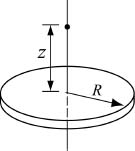
where σ is the charge density, ε₀ is the permittivity constant, ε₀ = 8.85 × 10⁻¹² C²/(N m²), and R is the radius of the disk. Determine the electric field at a point located 5 cm from a disk with a radius of 6 cm, charged with σ = 300 3956;C/m².

22.  The length of a curve given by a parametric equation x(t), y(t) is given by:

The cardioid curve shown in the figure is given by: x = 2b costt − b cos 2t, and y = 2b sint − b sin 2t with 0 ≤ t ≤ 2π. Plot the cardioid with b = 5 and determine the length of a the curve.

23.  The variation of gravitational acceleration g with altitude y is given by

where R = 6371 km is the radius of the earth, and g₀ = 9.81m/s² is the gravitational acceleration at sea level. The change in the gravitational potential energy, ΔU, of an object that is raised from the earth is given by:

Determine the change in the potential energy of a satellite with a mass of 500 kg that is raised from the surface of the earth to a height of 800 km.

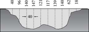
24.  A cross section of a river with measurements of its depth at intervals of 40 ft is shown in the figure. Use numerical integration to estimate the cross-sectional area of the river.

25.  An approximate map of the state of Texas is shown in the figure. For determining the area of the state, the map is divided into two parts (one above and one below the x axis). Determine the area of the state by numerically integrating the two areas. For each part make a list of the coordinate y of the border as a function of x. Start with x = 0 and use increments of 50 mi, such that the last point is x = 750. Compare the result with the actual area of Ohio, which is 261,797 square miles.

26.  A cross-sectional area has the geometry of half an ellipse, as shown in the figure to the right. The coordinate of the centroid of the area can be calculated by:

where A is the area given by , and M_y is the moment of the area about the y axis, given by:

Determine when a = 40 mm and b = 15 mm.

27.  The orbit of Pluto is elliptical in shape, with a = 5.9065 × 10⁹ km and b = 5.7208 × 10⁹ km. The perimeter of an ellipse can be calculated by

where . Determine the distance Pluto travels in one orbit. Calculate the average speed at which Pluto travels (in km/h) if one orbit takes about 248 years.

28.  The Fresnel integrals are:

Calculate s(x) and C(x) for 0 ≤ x ≤ 4 (use spacing of 0.05). In one figure plot two graphs—one of versus x and the other of C(x) versus x. In a second figure plot S(x) versus C(x).

29.  Use a MATLAB built-in function to numerically solve:

In one figure plot the numerical solution as a solid line and the exact solution as discrete points.

Exact solution: .

30.  Use a MATLAB built-in function to numerically solve:

In one figure plot the numerical solution as a solid line and the exact solution as discrete points.

Exact solution: .

31.  Use a MATLAB built-in function to numerically solve:

Plot the solution.

32.  Use a MATLAB built-in function to numerically solve:

Plot the solution.

33.  The growth of a fish is often modeled by the von Bertalanffy growth model:

where w is the weight and a and b are constants. Solve the equation for w for the case a = lb^1/3, b = 2 day^–1, and lb. Make sure that the selected time span is just long enough so that the maximum weight is approached. What is the maximum weight for this case? Make a plot of w as a function of time.

34.  A water tank shaped as an ellipsoid (a = 1.5 m, b = 4.0 m, c = 3m) has a circular hole at the bottom, as shown. According to Torricelli’s law, the speed v of the water that is discharging from the hole is given by

where h is the height of the water and g = 9.81 m/s². The rate at which the height, h, of the water in the tank changes as the water flows out through the hole is given by

where r_h is the radius of the hole.

Solve the differential equation for y. The initial height of the water is h = 5.9 m. Solve the problem for different times and find an estimate for the time when h = 0.1 m. Make a plot of y as a function of time.

35.  The sudden outbreak of an insect population can be modeled by the equation

The first term relates to the well-known logistic population growth model where N is the number of insects, R is an intrinsic growth rate, and C is the carrying capacity of the local environment. The second term represents the effects of bird predation. Its effect becomes significant when the population reaches a critical size N_c. r is the maximum value that the second term can reach at large values of N.

Solve the differential equation for 0 ≤ t ≤ 50 days and two growth rates, R = 0.55 and R = 0.58 day^–1, and with N(0) = 10000. The other parameters are C = 10⁴, N_c = 10⁴, r = 10⁴ day^–1. Make one plot comparing the two solutions and discuss why this model is called an “outbreak” model.

36.  An airplane uses a parachute and other means of braking as it slows down on the runway after landing. Its acceleration is given by a = −0.0035v² − 3 m/s². Since , the rate of change of the velocity is given by:

Consider an airplane with a velocity of 300 km/h that opens its parachute and starts decelerating at t = 0 s.

(a) By solving the differential equation, determine and plot the velocity as a function of time from t = 0 s until the airplane stops.

(b) Use numerical integration to determine the distance x the airplane travels as a function of time. Make a plot of x versus time.

37.  The population growth of species with limited capacity can be modeled by the equation:

where N is the population size, N_M is the limiting number for the population, and k is a constant. Consider the case where N_M = 5000, k = 0.000095 1/yr, and N(0) = 100. Determine N for 0 ≤ t ≤ 20. Make a plot of N as a function of t.

38.  An RL circuit includes a voltage source v_s, a resistor R = 1.8 Ω, and an inductor L = 0.4 H, as shown in the figure. The differential equation that describes the response of the circuit is

where i_L is the current in the inductor. Initially i_L = 0, and then at t = 0 the voltage source is changed. Determine the response of the circuit for the following three cases:

(a) v_s = 10sin(30πt) V for t ≥ 0.

(b) v_s = 10e^−t/0.06 sin(30πt) V for t ≥ 0.

Each case corresponds to a different differential equation. The solution is the current in the inductor as a function of time. Solve each case for 0 ≤ t ≤ 0.4 s. For each case plot v_s and i_L versus time (make two separate plots on the same page).

39.  Tumor growth can be modeled with the equation

where A(t) is the area of the tumor and α, k, and υ are constants. Solve the equation for 0 ≤ t ≤ 30 days, given α = 0.8, k = 60, υ = 0.25, and A(0) = 1 mm². Make a plot of A as a function of time.

40.  The velocity of an object that falls freely due to the earth gravity can be modeled by the equation:

where m is the mass of the object, g = 9.81 m/s², is and k is a constant. Solve the equation for v for the case m = 5 kg, k = 0.05 kg/m, 0 ≤ t ≤ 15 s and v(0) = 0 m/s. Make a plot of v as a function of time.