Despite the fact that everything varies, measurements often cluster around certain intermediate values; this attribute is called central tendency. Even if the data themselves do not show much tendency to cluster round some central value, the parameters derived from repeated experiments (e.g. replicated sample means) almost inevitably do (this is called the central limit theorem; see p. 70). We need some data to work with. The data are in a vector called y stored in a text file called yvalues

yvals <- read.csv("c:\temp\yvalues.csv")
attach(yvals)

So how should we quantify central tendency? Perhaps the most obvious way is just by looking at the data, without doing any calculations at all. The data values that occur most frequently are called the mode, and we discover the value of the mode simply by drawing a histogram of the data like this:

hist(y)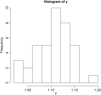

So we would say that the modal class of y was between 1.10 and 1.12 (we will see how to control the location of the break points in a histogram later).

The most straightforward quantitative measure of central tendency is the arithmetic mean of the data. This is the sum of all the data values divided by the number of data values, n. The capital Greek sigma just means ‘add up all the values’ of what follows; in this case, a set of y values. So if we call the arithmetic mean ‘y bar’, , we can write

The formula shows how we would write a general function to calculate arithmetic means for any vector of y values. First, we need to add them up. We could do it like this:

y[1] + y[2] + y[3] + . . . + y[n]

but that is very long-winded, and it supposes that we know the value of n in advance. Fortunately, there is a built-in function called sum that works out the total for any length of vector, so

total <- sum(y)

gives us the value for the numerator. But what about the number of data values? This is likely to vary from application to application. We could print out the y values and count them, but that is tedious and error-prone. There is a very important, general function in R to work this out for us. The function is called length(y) and it returns the number of numbers in the vector called y:

n <- length(y)

So our recipe for calculating the arithmetic mean would be ybar <- total/n.

ybar <- total/n

[1] 1.103464

There is no need to calculate the intermediate values, total and n, so it would be more efficient to write ybar <- sum(y)/length(y). To put this logic into a general function we need to pick a name for the function, say arithmetic.mean, then define it as follows:

arithmetic.mean <- function(x) sum(x)/length(x)

Notice two things: we do not assign the answer sum(x)/length(x) to a variable name like ybar; and the name of the vector x used inside the function(x) may be different from the names on which we might want to use the function in future (y, for instance). If you type the name of a function on its own, you get a listing of the contents:

arithmetic.mean

function(x) sum(x)/length(x)

Now we can test the function on some data. First we use a simple data set where we know the answer already, so that we can check that the function works properly: say

data <- c(3,4,6,7)

where we can see immediately that the arithmetic mean is 5.

arithmetic.mean(data)

[1] 5

So that's OK. Now we can try it on a realistically big data set:

arithmetic.mean(y)

[1] 1.103464

You will not be surprised to learn that R has a built-in function for calculating arithmetic means directly, and again, not surprisingly, it is called mean. It works in the same way as did our home-made function:

mean(y)

[1] 1.103464

Arithmetic mean is not the only quantitative measure of central tendency, and in fact it has some rather unfortunate properties. Perhaps the most serious failing of the arithmetic mean is that it is highly sensitive to outliers. Just a single extremely large or extremely small value in the data set will have a big effect on the value of the arithmetic mean. We shall return to this issue later, but our next measure of central tendency does not suffer from being sensitive to outliers. It is called the median, and is the ‘middle value’ in the data set. To write a function to work out the median, the first thing we need to do is sort the data into ascending order:

sorted <- sort(y)

Now we just need to find the middle value. There is slight hitch here, because if the vector contains an even number of numbers, then there is no middle value. Let us start with the easy case where the vector contains an odd number of numbers. The number of numbers in the vector is given by length(y)and the middle value is half of this:

length(y)/2

[1] 19.5

So the median value is the 20th value in the sorted data set. To extract the median value of y we need to use 20 as a subscript, not 19.5, so we should convert the value of length(y)/2 into an integer. We use ceiling (‘the smallest integer greater than’) for this:

ceiling(length(y)/2)

[1] 20

So now we can extract the median value of y:

sorted[20]

[1] 1.108847

or, more generally:

sorted[ceiling(length(y)/2)]

[1] 1.108847

or even more generally, omitting the intermediate variable called sorted:

sort(y)[ceiling(length(y)/2)]

[1] 1.108847

But what about the case where the vector contains an even number of numbers? Let us manufacture such a vector, by dropping the first element from our vector called y using negative subscripts like this:

y.even <- y[-1]

length(y.even)

[1] 38

The logic is that we shall work out the arithmetic average of the two values of y on either side of the middle; in this case, the average of the 19th and 20th sorted values:

sort(y.even)[19]

[1] 1.108847

sort(y.even)[20]

[1] 1.108853

So in this case, the median would be:

(sort(y.even)[19]+sort(y.even)[20])/2

[1] 1.10885

But to make it general we need to replace the 19 and 20 by

ceiling(length(y.even)/2)

and

ceiling(1+length(y.even)/2)

respectively.

The question now arises as to how we know, in general, whether the vector y contains an odd or an even number of numbers, so that we can decide which of the two methods to use. The trick here is to use ‘modulo’. This is the remainder (the amount ‘left over’) when one integer is divided by another. An even number has modulo 0 when divided by 2, and an odd number has modulo 1. The modulo function in R is %% (two successive percent symbols) and it is used where you would use slash / to carry out a regular division. You can see this in action with an even number, 38, and odd number, 39:

38%%2

[1] 0

39%%2

[1] 1

Now we have all the tools we need to write a general function to calculate medians. Let us call the function med and define it like this:

med <- function(x) {
modulo <- length(x)%%2
if (modulo == 0)  (sort(x)[ceiling(length(x)/2)]+sort(x)[ceiling(1+length(x)/2)])/2
else  sort(x)[ceiling(length(x)/2)]
}

Notice that when the if statement is true (i.e. we have an even number of numbers) then the expression immediately following the if statement is evaluated (this is the code for calculating the median with an even number of numbers). When the if statement is false (i.e. we have an odd number of numbers, and modulo == 1) then the expression following the else statement is evaluated (this is the code for calculating the median with an odd number of numbers). Let us try it out, first with the odd-numbered vector y, then with the even-numbered vector y.even, to check against the values we obtained earlier.

med(y)
[1] 1.108847
med(y.even)
[1] 1.10885

Both of these check out. Again, you will not be surprised that there is a built-in function for calculating medians, and helpfully it is called median:

median(y)
[1] 1.108847
median(y.even)
[1] 1.10885

For processes that change multiplicatively rather than additively, then neither the arithmetic mean nor the median is an ideal measure of central tendency. Under these conditions, the appropriate measure is the geometric mean. The formal definition of this is somewhat abstract: the geometric mean is the nth root of the product of the data. If we use capital Greek pi (∏) to represent multiplication, and y ‘hat’ () to represent the geometric mean, then

Let us take a simple example we can work out by hand: the numbers of insects on five different plants were as follows: 10, 1, 1000, 1, 10. Multiplying the numbers together gives 100 000. There are five numbers, so we want the fifth root of this. Roots are hard to do in your head, so we will use R as a calculator. Remember that roots are fractional powers, so the fifth root is a number raised to the power 1/5 = 0.2. In R, powers are denoted by the ^ symbol (the caret), which is found above number 6 on the keyboard:

100000^0.2

[1] 10

So the geometric mean of these insect numbers is 10 insects per stem. Note that two of the five counts were exactly this number, so it seems a reasonable estimate of central tendency. The arithmetic mean, on the other hand, is hopeless for these data, because the large value (1000) is so influential: 10 + 1 + 1000 + 1 + 10 = 1022 and 1022/5 = 204.4. Note that none of the counts were close to 204.4, so the arithmetic mean is a poor estimate of central tendency in this case.

insects <- c(1,10,1000,10,1)
mean(insects)

[1] 204.4

Another way to calculate geometric mean involves the use of logarithms. Recall that to multiply numbers together we add up their logarithms. And to take roots, we divide the logarithm by the root. So we should be able to calculate a geometric mean by finding the antilog (exp) of the average of the logarithms (log) of the data:

exp(mean(log(insects)))

[1] 10

Writing a general function to compute geometric means is left to you as an exercise.

The use of geometric means draws attention to a general scientific issue. Look at the figure below, which shows numbers varying through time in two populations. Now ask yourself ‘Which population is the more variable?’ Chances are, you will pick the upper line:

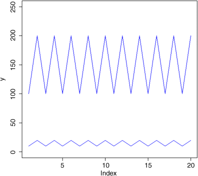
But now look at the scale on the y axis. The upper population is fluctuating 100, 200, 100, 200 and so on. In other words, it is doubling and halving, doubling and halving. The lower curve is fluctuating 10, 20, 10, 20, 10, 20 and so on. It, too, is doubling and halving, doubling and halving. So the answer to the question is: ‘They are equally variable’. It is just that one population has a higher mean value than the other (150 vs. 15 in this case). In order not to fall into the trap of saying that the upper curve is more variable than the lower curve, it is good practice to graph the logarithms rather than the raw values of things like population sizes that change multiplicatively.

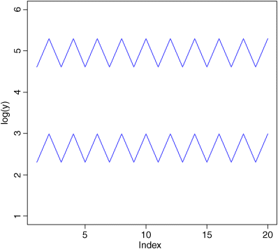
Now it is clear that both populations are equally variable.

Finally, we should deal with a rather different measure of central tendency. Consider the following problem. An elephant has a territory which is a square of side 2 km. Each morning, the elephant walks the boundary of this territory. It begins the day at a sedate pace, walking the first side of the territory at a speed of 1 km/hr. On the second side, he has sped up to 2 km/hr. By the third side he has accelerated to an impressive 4 km/hr, but this so wears him out, that he has to return on the final side at a sluggish 1 km/hr. So what is his average speed over the ground? You might say he travelled at 1, 2, 4 and 1 km/hr so the average speed is (1 + 2 + 4 + 1)/4 = 8/4 = 2 km/hr. But that is wrong. Can you see how to work out the right answer? Recall that velocity is defined as distance travelled divided by time taken. The distance travelled is easy: it is just 4 × 2 = 8 km. The time taken is a bit harder. The first edge was 2 km long and, travelling at 1 km/hr, this must have taken 2 hr. The second edge was 2 km long and, travelling at 2 km/hr, this must have taken 1 hr. The third edge was 2 km long and, travelling at 4 km/hr, this must have taken 0.5 hr. The final edge was 2 km long and, travelling at 1 km/hr, this must have taken 2 hr. So the total time taken was 2 + 1 + 0.5 + 2 = 5.5 hr. So the average speed is not 2 km/hr but 8/5.5 = 1.4545 km/hr.

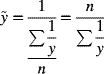
The way to solve this problem is to use the HARMONIC MEAN. This is the reciprocal of the average of the reciprocals. Remember that a reciprocal is ‘one over’. So the average of our reciprocals is . The reciprocal of this average is the harmonic mean . In symbols, therefore, the harmonic mean, , (y ‘curl’) is given by

In R, we would write either

v <- c(1,2,4,1)
length(v)/sum(1/v)

[1] 1.454545

or

1/mean(1/v)

[1] 1.454545