
10
Multiple Regression
In multiple regression we have a continuous response variable and two or more continuous explanatory variables (i.e. there are no categorical explanatory variables). In many applications, multiple regression is the most difficult of all the statistical models to do well. There are several things that make multiple regression so challenging:
- the studies are often observational (rather than controlled experiments)
- we often have a great many explanatory variables
- we often have rather few data points
- missing combinations of explanatory variables are commonplace
There are several important statistical issues, too:
- the explanatory variables are often correlated with one another (non-orthogonal)
- there are major issues about which explanatory variables to include
- there could be curvature in the response to the explanatory variables
- there might be interactions between explanatory variables
- the last three issues all tend to lead to parameter proliferation
There is a temptation to become personally attached to a particular model. Statisticians call this ‘falling in love with your model’. It is as well to remember the following truths about models:
- all models are wrong
- some models are better than others
- the correct model can never be known with certainty
- the simpler the model, the better it is
Fitting models to data is the central function of R. The process is essentially one of exploration; there are no fixed rules and no absolutes. The object is to determine a minimal adequate model from the large set of potential models that might be used to describe the given set of data. In this book we discuss five types of model:
- the null model
- the minimal adequate model
- the current model
- the maximal model
- the saturated model
The stepwise progression from the saturated model (or the maximal model, whichever is appropriate) through a series of simplifications to the minimal adequate model is made on the basis of deletion tests; these are F tests, AIC, t tests or chi-squared tests that assess the significance of the increase in deviance that results when a given term is removed from the current model.
Models are representations of reality that should be both accurate and convenient. However, it is impossible to maximize a model's realism, generality and holism simultaneously, and the principle of parsimony (Occam's razor; see p. 8) is a vital tool in helping to choose one model over another. Thus, we would only include an explanatory variable in a model if it significantly improved the fit of a model. Just because we went to the trouble of measuring something, that does not mean we have to have it in our model. Parsimony says that, other things being equal, we prefer:
- a model with n – 1 parameters to a model with n parameters
- a model with k – 1 explanatory variables to a model with k explanatory variables
- a linear model to a model which is curved
- a model without a hump to a model with a hump
- a model without interactions to a model containing interactions between variables
Other considerations include a preference for models containing explanatory variables that are easy to measure over variables that are difficult or expensive to measure. Also, we prefer models that are based on a sound mechanistic understanding of the process over purely empirical functions.
Parsimony requires that the model should be as simple as possible. This means that the model should not contain any redundant parameters or factor levels. We achieve this by fitting a maximal model then simplifying it by following one or more of these steps:
- remove non-significant interaction terms
- remove non-significant quadratic or other non-linear terms
- remove non-significant explanatory variables
- group together factor levels that do not differ from one another
- in ANCOVA, set non-significant slopes of continuous explanatory variables to zero
subject, of course, to the caveats that the simplifications make good scientific sense, and do not lead to significant reductions in explanatory power.
Just as there is no perfect model, so there may be no optimal scale of measurement for a model. Suppose, for example, we had a process that had Poisson errors with multiplicative effects amongst the explanatory variables. Then, one must chose between three different scales, each of which optimizes one of three different properties:
- the scale of
 would give constancy of variance
 - the scale of
 would give approximately normal errors
 - the scale of ln(y) would give additivity
Thus, any measurement scale is always going to be a compromise, and you should choose the scale that gives the best overall performance of the model.
| Model | Interpretation |
| Saturated model | One parameter for every data point Fit: perfect Degrees of freedom: none Explanatory power of the model: none |
| Maximal model | Contains all (p) factors, interactions and covariates that might be of any interest. Many of the model's terms are likely to be insignificant Degrees of freedom: n − p − 1 Explanatory power of the model: it depends |
| Minimal adequate model | A simplified model with Fit: less than the maximal model, but not significantly so Degrees of freedom: n − p′ − 1 Explanatory power of the model: r2 = SSR/SSY |
| Null model | Just one parameter, the overall mean Fit: none; SSE = SSY Degrees of freedom: n − 1 Explanatory power of the model: none |
The Steps Involved in Model Simplification
There are no hard and fast rules, but the procedure laid out below works well in practice. With large numbers of explanatory variables, and many interactions and non-linear terms, the process of model simplification can take a very long time. But this is time well spent because it reduces the risk of overlooking an important aspect of the data. It is important to realize that there is no guaranteed way of finding all the important structures in a complex dataframe.
| Step | Procedure | Explanation |
| 1 | Fit the maximal model | Fit all the factors, interactions and covariates of interest. Note the residual deviance. If you are using Poisson or binomial errors, check for overdispersion and rescale if necessary |
| 2 | Begin model simplification | Inspect the parameter estimates using summary. Remove the least significant terms first, using update -, starting with the highest-order interactions |
| 3 | If the deletion causes an insignificant increase in deviance | Leave that term out of the model. Inspect the parameter values again. Remove the least significant term remaining |
| 4 | If the deletion causes a significant increase in deviance | Put the term back in the model using update + . These are the statistically significant terms as assessed by deletion from the maximal model |
| 5 | Keep removing terms from the model | Repeat steps 3 or 4 until the model contains nothing but significant terms. This is the minimal adequate model. If none of the parameters is significant, then the minimal adequate model is the null model |
Caveats
Model simplification is an important process, but it should not be taken to extremes. For example, the interpretation of deviances and standard errors produced with fixed parameters that have been estimated from the data should be undertaken with caution. Again, the search for ‘nice numbers’ should not be pursued uncritically. Sometimes there are good scientific reasons for using a particular number (e.g. a power of 0.66 in an allometric relationship between respiration and body mass). Again, it is much more straightforward, for example, to say that yield increases by 2 kg per hectare for every extra unit of fertilizer, than to say that it increases by 1.947 kg. Similarly, it may be preferable to say that the odds of infection increase 10-fold under a given treatment, rather than to say that the logits increase by 2.321 (without model simplification this is equivalent to saying that there is a 10.186-fold increase in the odds). It would be absurd, however, to fix on an estimate of 6 rather than 6.1 just because 6 is a whole number.
Order of Deletion
Remember that when explanatory variables are correlated (as they almost always are in multiple regression), order matters. If your explanatory variables are correlated with each other, then the significance you attach to a given explanatory variable will depend upon whether you delete it from a maximal model or add it to the null model. If you always test by model simplification then you won't fall into this trap.
The fact that you have laboured long and hard to include a particular experimental treatment does not justify the retention of that factor in the model if the analysis shows it to have no explanatory power. ANOVA tables are often published containing a mixture of significant and non-significant effects. This is not a problem in orthogonal designs, because sums of squares can be unequivocally attributed to each factor and interaction term. But as soon as there are missing values or unequal weights, then it is impossible to tell how the parameter estimates and standard errors of the significant terms would have been altered if the non-significant terms had been deleted. The best practice is this
- say whether your data are orthogonal or not
- present a minimal adequate model
- give a list of the non-significant terms that were omitted, and the deviance changes that resulted from their deletion
Readers can then judge for themselves the relative magnitude of the non-significant factors, and the importance of correlations between the explanatory variables.
The temptation to retain terms in the model that are ‘close to significance’ should be resisted. The best way to proceed is this. If a result would have been important if it had been statistically significant, then it is worth repeating the experiment with higher replication and/or more efficient blocking, in order to demonstrate the importance of the factor in a convincing and statistically acceptable way.
Carrying Out a Multiple Regression
For multiple regression, the approach recommended here is that before you begin modelling in earnest you do two things:
- use tree models to investigate whether there are complicated interactions
- use generalized additive models to investigate curvature
Let us begin with an example from air pollution studies. How is ozone concentration related to wind speed, air temperature and the intensity of solar radiation?
ozone.pollution <- read.csv("c:\temp\ozone.data.csv")attach(ozone.pollution)names(ozone.pollution)[1] "rad" "temp" "wind" "ozone"
In multiple regression, it is always a good idea to use the pairs function to look at all the correlations:
pairs(ozone.pollution,panel=panel.smooth)
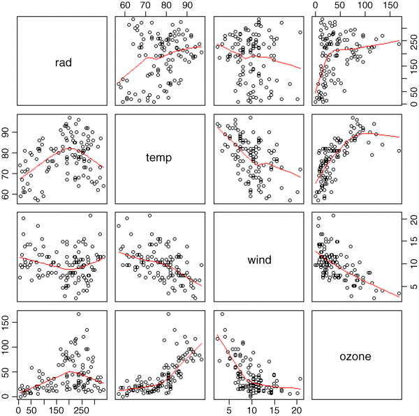
The response variable, ozone concentration, is shown on the y axis of the bottom row of panels: there is a strong negative relationship with wind speed, a positive correlation with temperature and a rather unclear, but possibly humped relationship with radiation.
A good way to start a multiple regression problem is using non-parametric smoothers in a generalized additive model (gam) like this:
library(mgcv)par(mfrow=c(2,2))model <- gam(ozone~s(rad)+s(temp)+s(wind))plot(model,col= "blue")
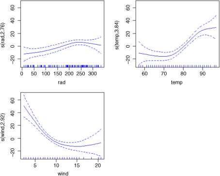
The confidence intervals are sufficiently narrow to suggest that the curvature in all three relationships might be real.
The next step might be to fit a tree model to see whether complex interactions between the explanatory variables are indicated. The older tree function is better for this graphical search for interactions than is the more modern rpart (but the latter is much better for statistical modelling):
par(mfrow=c(1,1))library(tree)model <- tree(ozone~.,data=ozone.pollution)plot(model)text(model)
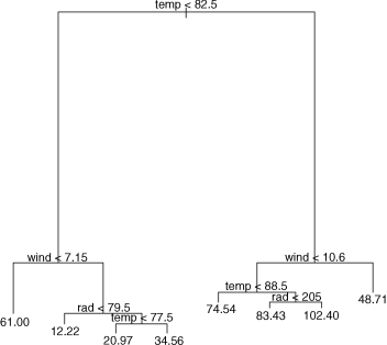
This shows that temperature is far and away the most important factor affecting ozone concentration (the longer the branches in the tree, the greater the deviance explained). Wind speed is important at both high and low temperatures, with still air being associated with higher mean ozone levels (the figures at the ends of the branches are mean ozone concentrations). Radiation shows an interesting, but subtle effect. At low temperatures, radiation matters at relatively high wind speeds (>7.15), whereas at high temperatures, radiation matters at relatively low wind speeds (<10.6); in both cases, however, higher radiation is associated with higher mean ozone concentration. The tree model therefore indicates that the interaction structure of the data is not particularly complex (this is a reassuring finding).
Armed with this background information (likely curvature of responses and a relatively uncomplicated interaction structure), we can begin the linear modelling. We start with the most complicated model: this includes interactions between all three explanatory variables plus quadratic terms to test for curvature in response to each of the three explanatory variables:
model1 <- lm(ozone~temp*wind*rad+I(rad^2)+I(temp^2)+I(wind^2))summary(model1)Coefficients:Estimate Std. Error t value Pr (>|t|)(Intercept) 5.683e+02 2.073e+02 2.741 0.00725 **temp -1.076e+01 4.303e+00 -2.501 0.01401 *wind -3.237e+01 1.173e+01 -2.760 0.00687 **rad -3.117e-01 5.585e-01 -0.558 0.57799I(rad^2) -3.619e-04 2.573e-04 -1.407 0.16265I(temp^2) 5.833e-02 2.396e-02 2.435 0.01668 *I(wind^2) 6.106e-01 1.469e-01 4.157 6.81e-05 ***temp:wind 2.377e-01 1.367e-01 1.739 0.08519 .temp:rad 8.403e-03 7.512e-03 1.119 0.26602wind:rad 2.054e-02 4.892e-02 0.420 0.67552temp:wind:rad -4.324e-04 6.595e-04 -0.656 0.51358Residual standard error: 17.82 on 100 degrees of freedomMultiple R-squared: 0.7394, Adjusted R-squared: 0.7133F-statistic: 28.37 on 10 and 100 DF, p-value: < 2.2e-16
The three-way interaction is clearly not significant, so we remove it to begin the process of model simplification:
model2 <- update(model1,~. – temp:wind:rad)summary(model2)
Next, we remove the least significant two-way interaction term, in this case wind:rad:
model3 <- update(model2,~. - wind:rad)summary(model3)
Then we try removing the temperature by wind interaction:
model4 <- update(model3,~. - temp:wind)summary(model4)
We shall retain the marginally significant interaction between temp and rad (p = 0.04578) for the time being, but leave out all other interactions. In model4, the least significant quadratic term is for rad, so we delete this:
model5 <- update(model4,~. - I(rad^2))summary(model5)
This deletion has rendered the temp:rad interaction insignificant, and caused the main effect of radiation to become insignificant. We should try removing the temp:rad interaction:
model6 <- update(model5,~. - temp:rad)summary(model6)Coefficients:Estimate Std. Error t value Pr (>|t|)(Intercept) 291.16758 100.87723 2.886 0.00473 **temp -6.33955 2.71627 -2.334 0.02150 *wind -13.39674 2.29623 -5.834 6.05e-08 ***rad 0.06586 0.02005 3.285 0.00139 **I(temp^2) 0.05102 0.01774 2.876 0.00488 **I(wind^2) 0.46464 0.10060 4.619 1.10e-05 ***Residual standard error: 18.25 on 105 degrees of freedomMultiple R-Squared: 0.713, Adjusted R-squared: 0.6994F-statistic: 52.18 on 5 and 105 DF, p-value: 0
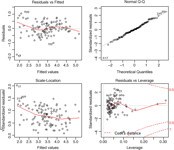
Now we are making progress. All the terms in model6 are significant. At this stage, we should check the assumptions, using plot(model6):
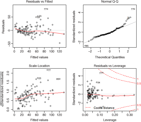
There is a clear pattern of variance increasing with the mean of the fitted values. This is bad news (heteroscedasticity). Also, the normality plot is distinctly curved; again, this is bad news. Let us try transformation of the response variable. There are no zeros in the response, so a log transformation is worth trying. We need to repeat the entire process of model simplification from the very beginning, because transformation alters the variance structure and the linearity of all the relationships.
model7 <- lm(log(ozone)~temp*wind*rad+I(rad^2)+I(temp^2)+I(wind^2))
We can speed up the model simplification using the step function:
model8 <- step(model7)summary(model8)Coefficients:Estimate Std. Error t value Pr(>|t|)(Intercept) 7.724e-01 6.350e-01 1.216 0.226543temp 4.193e-02 6.237e-03 6.723 9.52e-10 ***wind -2.211e-01 5.874e-02 -3.765 0.000275 ***rad 7.466e-03 2.323e-03 3.215 0.001736 **I(rad^2) -1.470e-05 6.734e-06 -2.183 0.031246 *I(wind^2) 7.390e-03 2.585e-03 2.859 0.005126 **Residual standard error: 0.4851 on 105 degrees of freedomMultiple R-squared: 0.7004, Adjusted R-squared: 0.6861F-statistic: 49.1 on 5 and 105 DF, p-value: < 2.2e-16
This simplified model following transformation has a different structure than before: all three main effects are significant and there are still no interactions between variables, but the quadratic term for temperature has gone and a quadratic term for radiation remains in the model. We need to check that transformation has improved the problems that we had with non-normality and non-constant variance:
plot(model8)
This shows that the variance and normality are now reasonably well behaved, so we can stop at this point. We have found the minimal adequate model. Our initial impressions from the tree model (no interactions) and the generalized additive model (a good deal of curvature) have been borne out by the statistical modelling.
A Trickier Example
In this example we introduce two new but highly realistic difficulties: more explanatory variables, and fewer data points. This is another air pollution dataframe, but the response variable this time is sulphur dioxide concentration. There are six continuous explanatory variables:
pollute <- read.csv("c:\temp\sulphur.dioxide.csv")attach(pollute)names(pollute)[1] "Pollution" "Temp" "Industry" "Population" "Wind"[6] "Rain" "Wet.days"
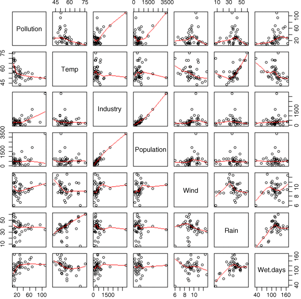
Here are the 36 paired scatterplots:
pairs(pollute,panel=panel.smooth)
This time, let us begin with the tree model rather than the generalized additive model.
par(mfrow=c(1,1))library(tree)model <- tree(Pollution~.,data=pollute)plot(model)text(model)
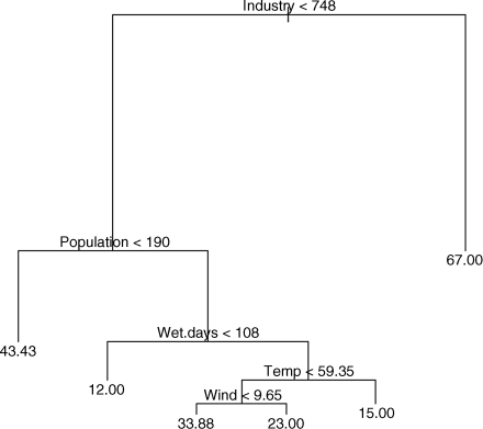
This tree model is much more complicated than we saw in the previous ozone example. It is interpreted as follows. The most important explanatory variable is industry, and the threshold value separating low and high values of industry is 748. The right hand branch of the tree indicates the mean value of air pollution for high levels of industry (67.00). The fact that this limb is unbranched means that no other variables explain a significant amount of the variation in pollution levels for high values of industry. The left-hand limb does not show the mean values of pollution for low values of industry, because there are other significant explanatory variables. Mean values of pollution are only shown at the extreme ends of branches. For low values of industry, the tree shows us that population has a significant impact on air pollution. At low values of population (< 190) the mean level of air pollution was 43.43. For high values of population, the number of wet days is significant. Low numbers of wet days (< 108) have mean pollution levels of 12.00, while temperature has a significant impact on pollution for places where the number of wet days is large. At high temperatures (> 59.35 °F) the mean pollution level was 15.00, while at lower temperatures the run of wind is important. For still air (wind < 9.65) pollution was higher (33.88) than for higher wind speeds (23.00).
The virtues of tree-based models are numerous:
- they are easy to appreciate and to describe to other people
- the most important variables stand out
- interactions are clearly displayed
- non-linear effects are captured effectively
- the complexity of the behaviour of the explanatory variables is plain to see
We conclude that the interaction structure is highly complex. We shall need to carry out the linear modelling with considerable care.
Start with some elementary calculations. With six explanatory variables, how many interactions might we fit? Well, there are 5 + 4 + 3 + 2 + 1 = 15 two-way interactions for a start. Plus 20 three-way, 15 four-way and 6 five-way interactions, and 1 six-way interaction for good luck. Then there are quadratic terms for each of the six explanatory variables. So we are looking at about 70 parameters that might be estimated from the data with a complete maximal model. But how many data points do we have?
length(Pollution)[1] 41
Oops! We are planning to estimate almost twice as many parameters as there are data points. That's taking over-parameterization to new heights. This leads us to a very general and extremely important question: how many data points does one need per parameter to be estimated?
Of course there can be no hard and fast answer to this, but perhaps there are some useful rules of thumb? To put the question another way, given that I have 41 data points, how many parameters is it reasonable to expect that I shall be able to estimate from the data?
As an absolute minimum, one would need at least three data points per parameter (remember that any two points can always be joined perfectly by a straight line). Applying this to our current example means that the absolute maximum we should try to estimate would be 41/3 = 13 parameters (one for the intercept plus 12 slopes). A more conservative rule of thumb might suggest 10 data points per parameter, under which more stringent criteria we would be allowed to estimate an intercept and just three slopes.
It is at this stage that the reality bites. If I cannot fit all of the explanatory variables I want, then how do I choose which ones to fit? This is a problem because:
- main effects can appear to be non-significant when a relationship is strongly curved (see p. 148) so if I don't fit a quadratic term (using up an extra parameter in the process) I shan't be confident about leaving a variable out of the model
- main effects can appear to be non-significant when interactions between two or more variables are pronounced (see p. 174)
- interactions can only be investigated when variables appear together in the same model (interactions between two continuous explanatory variables are typically included in the model as a function of the product of the two variables, and both main effects should be included when we do this)
The ideal strategy is to fit a maximal model containing all the explanatory variables, with curvature terms for each variable, along with all possible interactions terms, and then simplify this maximal model, perhaps using step to speed up the initial stages. In our present example, however, this is completely out of the question. We have far too many variables and far too few data points.
In this example, it is impossible to fit all combinations of variables simultaneously and hence it is highly likely that important interaction terms could be overlooked. We know from the tree model that the interaction structure is going to be complicated, so we need to concentrate on that. Perhaps a good place to start is by looking for curvature, to see if we can eliminate this as a major cause of variation. Fitting all the variables and their quadratic terms requires an intercept and 12 slopes to be estimated, and this is right at the extreme limit of three data points per parameter:
model1 <- lm(Pollution~Temp+I(Temp^2)+Industry+I(Industry^2)+Population+I(Population^2)+Wind+I(Wind^2)+Rain+I(Rain^2)+Wet.days+I(Wet.days^2))summary(model1)Coefficients:Estimate Std. Error t value Pr (>|t|)(Intercept) -6.641e+01 2.234e+02 -0.297 0.76844Temp 5.814e-01 6.295e+00 0.092 0.92708I(Temp^2) -1.297e-02 5.188e-02 -0.250 0.80445Industry 8.123e-02 2.868e-02 2.832 0.00847 **I(Industry^2) -1.969e-05 1.899e-05 -1.037 0.30862Population -7.844e-02 3.573e-02 -2.195 0.03662 *I(Population^2) 2.551e-05 2.158e-05 1.182 0.24714Wind 3.172e+01 2.067e+01 1.535 0.13606I(Wind^2) -1.784e+00 1.078e+00 -1.655 0.10912Rain 1.155e+00 1.636e+00 0.706 0.48575I(Rain^2) -9.714e-03 2.538e-02 -0.383 0.70476Wet.days -1.048e+00 1.049e+00 -0.999 0.32615I(Wet.days^2) 4.555e-03 3.996e-03 1.140 0.26398Residual standard error: 14.98 on 28 degrees of freedomMultiple R-squared: 0.7148, Adjusted R-squared: 0.5925F-statistic: 5.848 on 12 and 28 DF, p-value: 5.868e-05
So that's our first bit of good news. In this unsimplified model, there is no evidence of curvature for any of the six explanatory variables. Only the main effects of industry and population are significant in this (highly over-parameterized) model. Let us see what step makes of this:
model2 <- step(model1)summary(model2)Coefficients:Estimate Std. Error t value Pr(>|t|)(Intercept) 54.468341 14.448336 3.770 0.000604 ***I(Temp^2) -0.009525 0.003395 -2.805 0.008150 **Industry 0.065719 0.015246 4.310 0.000126 ***Population -0.040189 0.014635 -2.746 0.009457 **I(Wind^2) -0.165965 0.089946 -1.845 0.073488 .Rain 0.405113 0.211787 1.913 0.063980 .Residual standard error: 14.25 on 35 degrees of freedomMultiple R-squared: 0.6773, Adjusted R-squared: 0.6312F-statistic: 14.69 on 5 and 35 DF, p-value: 8.951e-08
The simpler model shows significant curvature of temperature and marginally significant curvature for wind. Notice that step has removed the linear terms for Temp and Wind; normally when we have a quadratic term we retain the linear term even if its slope is not significantly different from zero. Let us remove the non-significant terms from model2 to see what happens:
model3 <- update(model2, ~.- Rain-I(Wind^2))summary(model3)Coefficients:Estimate Std. Error t value Pr (>|t|)(Intercept) 42.068701 9.993087 4.210 0.000157 ***I(Temp^2) -0.005234 0.003100 -1.688 0.099752 .Industry 0.071489 0.015871 4.504 6.45e-05 ***Population -0.046880 0.015199 -3.084 0.003846 **Residual standard error: 15.08 on 37 degrees of freedomMultiple R-squared: 0.6183, Adjusted R-squared: 0.5874F-statistic: 19.98 on 3 and 37 DF, p-value: 7.209e-08
Simplification reduces the significance of the quadratic term for temperature. We shall need to return to this. The model supports out interpretation of the initial tree model: a main effect for industry is very important, as is a main effect for population.
Now we need to consider the interaction terms. We shall not fit interaction terms without both the component main effects, so we cannot fit all the two-way interaction terms at the same time (that would be 15 + 6 = 21 parameters; well above the rule of thumb maximum value of 13). One approach is to fit the interaction terms in randomly selected sets. With all six main effects, we can afford to assess 13 − 6 = 7 interaction terms at a time. Let us try this. Make a vector containing the names of the 15 two-way interactions:
interactions <- c("ti","tp","tw","tr","td","ip","iw","ir","id","pw","pr","pd","wr","wd","rd")
Now shuffle the interactions into random order using sample without replacement:
sample(interactions)[1] "wr" "wd" "id" "ir" "rd" "pr" "tp" "pw" "ti"[10]"iw" "tw" "pd" "tr" "td" "ip"
It would be pragmatic to test the two-way interactions in three models each containing all the main effects, plus two-way interaction terms five-at-a-time:
model4 <- lm(Pollution~Temp+Industry+Population+Wind+Rain+Wet.days+Wind:Rain+Wind:Wet.days+Industry:Wet.days+Industry:Rain+Rain:Wet.days)model5 <- lm(Pollution~Temp+Industry+Population+Wind+Rain+Wet.days+Population:Rain+Temp:Population+Population:Wind+Temp:Industry+Industry:Wind)model6 <- lm(Pollution~Temp+Industry+Population+Wind+Rain+Wet.days+Temp:Wind+Population:Wet.days+Temp:Rain+Temp:Wet.days+Industry:Population)
Extracting only the interaction terms from the three models, we see:
Industry:Rain -1.616e-04 9.207e-04 -0.176 0.861891Industry:Wet.days 2.311e-04 3.680e-04 0.628 0.534949Wind:Rain 9.049e-01 2.383e-01 3.798 0.000690 ***Wind:Wet.days -1.662e-01 5.991e-02 -2.774 0.009593 **Rain:Wet.days 1.814e-02 1.293e-02 1.403 0.171318Temp:Industry -1.643e-04 3.208e-03 -0.051 0.9595Temp:Population 1.125e-03 2.382e-03 0.472 0.6402Industry:Wind 2.668e-02 1.697e-02 1.572 0.1267Population:Wind -2.753e-02 1.333e-02 -2.066 0.0479 *Population:Rain 6.898e-04 1.063e-03 0.649 0.5214Temp:Wind 1.261e-01 2.848e-01 0.443 0.66117Temp:Rain -7.819e-02 4.126e-02 -1.895 0.06811 .Temp:Wet.days 1.934e-02 2.522e-02 0.767 0.44949Industry:Population 1.441e-06 4.178e-06 0.345 0.73277Population:Wet.days 1.979e-05 4.674e-04 0.042 0.96652
The next step might be to put all of the significant or close-to-significant interactions into the same model, and see which survive:
model7 <- lm(Pollution~Temp+Industry+Population+Wind+Rain+Wet.days+Wind:Rain+Wind:Wet.days+Population:Wind+Temp:Rain)summary(model7)Coefficients:Estimate Std. Error t value Pr (>|t|)(Intercept) 323.054546 151.458618 2.133 0.041226 *Temp -2.792238 1.481312 -1.885 0.069153 .Industry 0.073744 0.013646 5.404 7.44e-06 ***Population 0.008314 0.056406 0.147 0.883810Wind -19.447031 8.670820 -2.243 0.032450 *Rain -9.162020 3.381100 -2.710 0.011022 *Wet.days 1.290201 0.561599 2.297 0.028750 *Temp:Rain 0.017644 0.027311 0.646 0.523171Population:Wind -0.005684 0.005845 -0.972 0.338660Wind:Rain 0.997374 0.258447 3.859 0.000562 ***Wind:Wet.days -0.140606 0.053582 -2.624 0.013530 *
We certainly don't need Temp:Rain
or Population:Windmodel8 <- update(model7,~.-Temp:Rain)summary(model8)
model9 <- update(model8,~.-Population:Wind)summary(model9)Coefficients:Estimate Std. Error t value Pr (>|t|)(Intercept) 290.12137 71.14345 4.078 0.000281 ***Temp -2.04741 0.55359 -3.698 0.000811 ***Industry 0.06926 0.01268 5.461 5.19e-06 ***Population -0.04525 0.01221 -3.707 0.000793 ***Wind -20.17138 5.61123 -3.595 0.001076 **Rain -7.48116 1.84412 -4.057 0.000299 ***Wet.days 1.17593 0.54137 2.172 0.037363 *Wind:Rain 0.92518 0.20739 4.461 9.44e-05 ***Wind:Wet.days -0.12925 0.05200 -2.486 0.018346 *Residual standard error: 11.75 on 32 degrees of freedomMultiple R-squared: 0.7996, Adjusted R-squared: 0.7495F-statistic: 15.96 on 8 and 32 DF, p-value: 3.51e-09All the terms in model7 are significant. Time for a check on the behaviour of the model:
There are two significant two-way interactions, Wind:Rain and Wind:Wet.days. It is time to check the assumptions:
plot(model9)
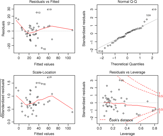
The variance is OK, but there is a strong indication of non-normality of errors. But what about the higher-order interactions? One way to proceed is to specify the interaction level using ^3 in the model formula, but if we do this, we'll run out of degrees of freedom straight away. A sensible option is to fit three-way terms for the variables that already appear in two-way interactions: in our case, that is just one term, Wind:Rain:Wet.days:
model10 <- update(model9,~. + Wind:Rain:Wet.days)summary(model10)Coefficients:Estimate Std. Error t value Pr (>|t|)(Intercept) 278.464474 68.041497 4.093 0.000282 ***Temp -2.710981 0.618472 -4.383 0.000125 ***Industry 0.064988 0.012264 5.299 9.11e-06 ***Population -0.039430 0.011976 -3.293 0.002485 **Wind -7.519344 8.151943 -0.922 0.363444Rain -6.760530 1.792173 -3.772 0.000685 ***Wet.days 1.266742 0.517850 2.446 0.020311 *Wind:Rain 0.631457 0.243866 2.589 0.014516 *Wind:Wet.days -0.230452 0.069843 -3.300 0.002440 **Wind:Rain:Wet.days 0.002497 0.001214 2.056 0.048247 *Residual standard error: 11.2 on 31 degrees of freedomMultiple R-squared: 0.8236, Adjusted R-squared: 0.7724F-statistic: 16.09 on 9 and 31 DF, p-value: 2.231e-09
There is indeed a marginally significant three-way interaction. You should confirm that there is no place for quadratic terms for either Temp or Wind in this model.
That's enough for now. I'm sure you get the idea. Multiple regression is difficult, time-consuming, and always vulnerable to subjective decisions about what to include and what to leave out. The linear modelling confirms the early impression from the tree model: for low levels of industry, the SO2 level depends in a simple way on population (people tend to want to live where the air is clean) and in a complicated way on daily weather (as reflected by the three-way interaction between wind, total rainfall and the number of wet days (i.e. on rainfall intensity)).
Further Reading
- Claeskens, G. and Hjort, N.L. (2008) Model Selection and Model Averaging, Cambridge University Press, Cambridge.
- Draper, N.R. and Smith, H. (1981) Applied Regression Analysis, John Wiley & Sons, New York.
- Fox, J. (2002) An R and S-Plus Companion to Applied Regression, Sage, Thousand Oaks, CA.
- Mosteller, F. and Tukey, J.W. (1977) Data Analysis and Regression, Addison-Wesley, Reading, MA.