Chapter 9
Cash Flow Profiles and Valuation Procedures
9.1 FROM BUSINESS MODELS TO CASH FLOW MODELS
The aim of this chapter is to show that financial valuation methods produce reliable estimates if and only if a specific in-depth business analysis is performed. Such an analysis has to embrace not only strategic and competitive aspects, which are the basis for any valuation task, but also financial dynamics, including the debt profile over time. Such analyses allow the expert to define the most suitable cash flow valuation method to be applied in any specific case. In particular, the analyst has to decide whether to use the aggregated versus the disaggregated approach, and on the treatment of the tax advantages of debt.
Before starting the discussion, it is worth focusing on the analytical process that precedes the final stage of a valuation, that is, the application of a discounted cash flow formula. Exhibit 9.1 summarizes the different necessary steps to better understand the background of the company or project under consideration.
Exhibit 9.1 Understanding the business model and choosing a valuation procedure
|
|
|
|
|
|
|
When valuing a company, a potential issue lies in the fact that standard plan horizons, usually around three to five years long or slightly longer, only explain a small portion of total firm's value. In fact, the bulk of the value is a function of the long-term results obtained beyond the standard plan horizons. It is therefore necessary to define a cash flow model that matches not only the financial dynamics of the medium-term (three to five years) forecasts, but also the assumptions made for the longer-term analysis.
9.2 CASH FLOW PROFILES OF BUSINESS UNITS VERSUS WHOLE ENTITY
If at a multi-business company the business units are independent enough on an operational basis, it could be worthwhile to develop specific cash flow projections and specific assumptions beyond the standard plan horizon for each business area. This estimation process is often referred to by the international community as the sum-of-parts (SOP) approach.
It is important to note that an SOP valuation could sometimes prove to be meaningless. As a matter of fact, horizontal synergies between areas are often such an important element that a comprehensive analysis and valuation is necessary. For instance, when evaluating “multi-utility” companies, it is meaningless to try and assign the existing synergies across different services to a specific business area (i.e., energy, electricity, water). Therefore, in order to choose the most appropriate valuation process, we should follow these steps:
- Look for potential surplus assets or surplus businesses.
- Look for autonomously profitable business units.
- Look for business activities that are best analyzed as a whole due to operations' synergies.
- Analyze the cash flows of the relevant units.
Therefore, the total company value when the company operates in more than one business is obtained as in Exhibit 9.2.
Exhibit 9.2 Multi-business company valuation
| Surplus assets | |
| Specific business areas value (asset value) | |
| Aggregated businesses value (asset value) | |
| Total asset value | |
| Financial (net) debt | |
| Equity value |
9.3 EXAMPLES OF CASH FLOW PROFILES
This section presents some typical cash flow profiles related to EBITDA and FCFO throughout the standard three to five years forecasted plan as well as in the phase beyond that. The choice between EBITDA and FCFO has already been addressed at the beginning of this book and it mainly resides in the level of investments in fixed assets and working capital (and in the related taxes).
Exhibits 9.3 and 9.4 present the cash flow profiles of two public utility companies: one in the natural gas distribution business (Exhibit 9.3) and the other in the hydroelectric generation business (Exhibit 9.4).
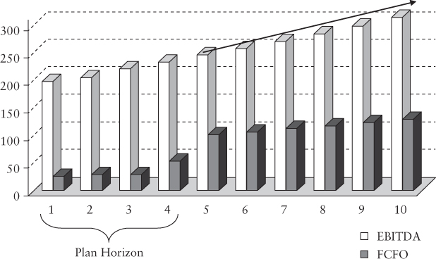
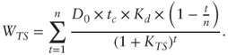
Exhibit 9.3 Cash flow examples: public utility (natural gas distribution)
During the plan horizon, the cash flow of the energy company mirrors the consumption growth associated with new industrial and local client base. Beyond the plan horizon, the FCFO is significantly greater than the FCFO of the final year of the plan horizon (year 4). This is due to the lower long-term growth assumptions both for the expansion of current pipelines and for new acquisitions.
The development of the flow beyond the plan horizon is based on two major assumptions:
- A consumption growth rate in line with the GDP growth rate
- A price to customers that guarantees the full remuneration of invested capital
At this point, it is worth highlighting that the cash flows considered so far are expressed in nominal terms—that is, they include the expected increase in prices.
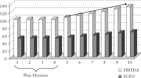
Exhibit 9.4 Cash flow examples: public utility (hydroelectric)
Exhibit 9.4 shows an even simpler case. It represents a company running a hydroelectric power plant. Some of the assumptions are that there is neither the need for extraordinary investments nor the necessity to expand the production capacity. Therefore, the cash flows beyond the plan horizon only grow due to an increase in (regulated) prices mirroring an increase in costs.
As previously stated, the EBITDA is systematically greater than the FCFO. This is due to the fact that the operating cash flow is computed by subtracting the amounts of maintenance investments and taxes from the EBITDA.
Exhibit 9.5 refers to the launch of “print on demand” services for a company in the printing industry. The EBITDA and the FCFO trends during the plan horizon are similar to those of a typical start-up: negative financial results in the first years are followed by a development and expansion phase. In this case, the financial profile is a result of the necessary investments in fixed assets and promotional activities. At the end of the plan horizon, growth is assumed to stop due to the entry of new competitors in the same business area. The decrease in profit margins due to the increase in competition should nevertheless take into account the impact of inflation on cash flow.
Exhibit 9.5 Cash flow examples: print on demand
Exhibit 9.6 shows the cash flow profiles of a company operating in the waste management industry—a landfill, to be precise. Differently from previous scenarios discussed, this venture has a limited life, as the landfill capacity is limited. The flow is simply determined by valuing the waste annually treated on the basis of average margins.
The financial representation (FCFO) highlights that, at the end of the investment's life, the flow is negative. This is due to the need for a new drainage system required to comply with safety regulations.
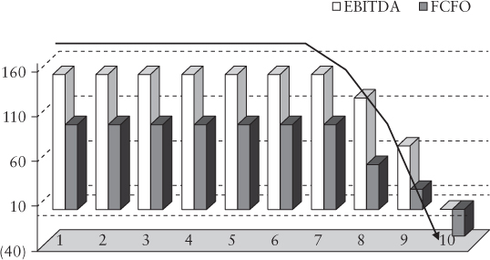
Exhibit 9.6 Cash flow profile examples: waste management company
Exhibit 9.7 illustrates the cash flow projections in industries affected by cyclical dynamics (iron and steel industries). The dashed arrow represents the profile of the cycle projected on the basis of forecasts made by industry experts.
The specific problems for this valuation procedure are not related to the plan's forecast period but to the estimate of a standardized result of long-term cash flows that adequately incorporates the cycle dynamics.
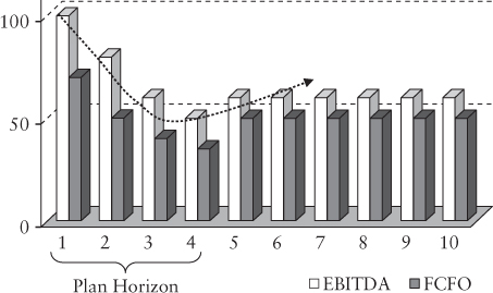
Exhibit 9.7 Cash flow profiles: cyclical sector
A common solution used by financial analysts is to estimate the EBITDA and the FCFO values consistent with a standard scenario based on historical industry performance.
In this specific example, the plan horizon ends with the downturn phase of the cycle. The cash flows used to estimate the terminal value therefore hypothesize an average scenario where the highest results are balanced with the lowest ones. It is assumed afterward that the normalized flow can be projected onto an infinite horizon.
Finally, Exhibit 9.8 shows a bank's cash flow profile. The analysis is carried out in distinct business areas. In this specific case, in addition to the bank's lending activity, there are new businesses with growth perspectives, risk profiles, and capital commitments different from those of the traditional banking activity.
Historical data confirm the high correlation between GDP growth and the bank's traditional business growth. Thus, the traditional lending business is a mature business with a relatively “flat” cash flow profile.
The portfolio management business has a higher growth potential in the short term. However, the growth pace is expected to slow down once the activity reaches a point of competitive equilibrium. As a consequence, the cash flow profiles will eventually grow at a slower pace, showing a high growth rate only for a limited number of years (as shown in Exhibit 9.9).
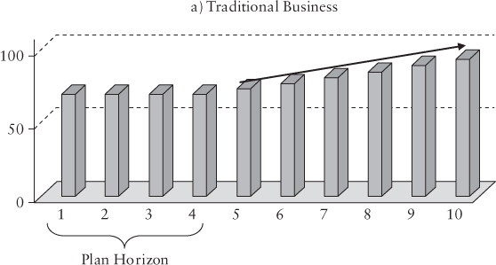
Exhibit 9.8 Cash flow profiles: savings and loans (traditional business)
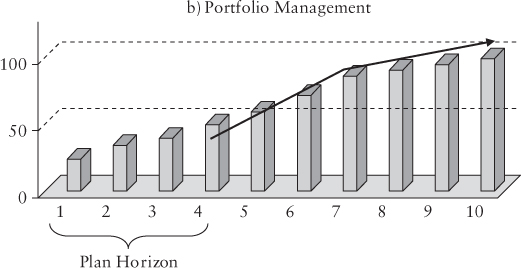
Exhibit 9.9 Cash flow profiles: savings and loans (portfolio management)
On the other end, in this specific example, the investment banking business has interesting growth potential in the medium term. The growth for this specific business has been limited to the plan horizon due to an expected high level of competition and to the cyclical evolution characterizing the investment banking business as a whole (see Exhibit 9.10).
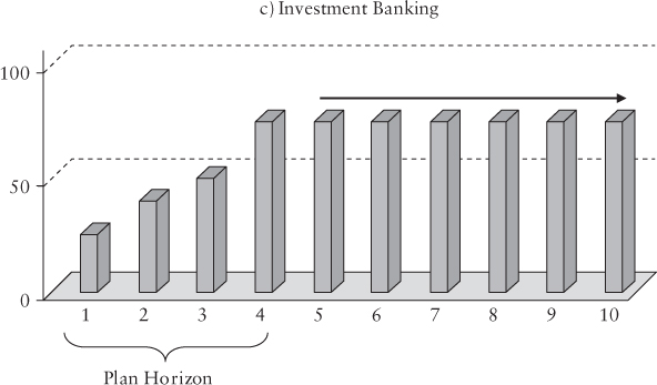
Exhibit 9.10 Cash flow profiles: savings and loans (investment banking)
9.4 PROBLEMS WITH THE IDENTIFICATION OF CASH FLOW MODELS
We have highlighted that one of the key tasks in a valuation is the assessment of company's business model.
The business model credibility is also an important condition to sustain cash flow projections. There are at least two scenarios in which it is extremely difficult, or even impossible, to build a reliable cash flow model:
- Companies lacking a distinctive competitive advantage in terms of strategic or operational resources.
- Captive companies—that is, companies that are incapable of standing autonomously on the market because they heavily depend on one or a few clients.
If such conditions are met, the long-term cash flow profile tends to be highly unpredictable and a mere function of exogenous random factors.
Therefore, the stand-alone valuation of a captive company or of a company without distinctive characteristics should be based on the assumption that it is possible to gather the necessary resources to allow the company to stay and compete autonomously in the market.
9.5 CASH FLOW MODELS IN THE CASE OF RESTRUCTURING
All firms undergoing a restructuring process share two important characteristics:
- Throughout the plan horizon, the company's financial dynamics mirror the restructuring process, which could lead to the divestment of surplus assets or of entire business units. Changes in the working capital can also significantly influence the cash flow profile.
- At the end of the plan, the long-term cash flow profile is based on the likelihood of success of the restructuring as well as on the changes made to keep the key business resources.
Thus, the cash flow credibility depends on the credibility of the restructuring objectives. Due to the importance of future events, different assumptions are usually taken into consideration by using sensitivity analysis and by looking into alternative scenarios.
9.6 DEBT PROFILE ANALYSIS
Debt profile analysis has the following purposes:
- The identification of a realistic model for the pattern of the company's net financial debt
- The valuation of tax shields consistently with the debt profile used in the estimation process
To facilitate the discussion, we will split the problem into two parts, separating the debt profile held during the period covered by the business plan from the debt profile (or its projection) in the period beyond the plan.
9.6.1 Debt Profile in the Business Plan Horizon Forecast
The debt profile analysis during the plan horizon requires the availability of complete economic and financial projections. Therefore the plan should show the expected evolution of the equity capital and of the financial structure. This means that it will also be necessary to estimate the dividend distribution patterns since they impact the level of financial leverage.
The easiest and most transparent valuation process usually includes the independent estimation of tax shields. This is due to the fact that, during the plan horizon, debt follows dynamics determined by the cash flow generated by the business, the debt repayment plan, and the dividend policy. On the other hand, the use of the aggregated valuation method (discounting the FCFO at the WACC*) is questionable, as it gives approximate results.
Exhibit 9.11 highlights the results for a listed company as estimated by a major investment bank. The expert has integrated the four-year business plan with a three-year projection period in order to verify the debt dynamics and the tax benefits associated with leverage. The analyst concluded that, given the same dividend policy and with no buyback deals, the cash flow would allow the complete repayment of the existing debt.
Exhibit 9.11 Relevant forecasts in evaluating WTS (mln / €)
| t1 | t2 | t3 | t4 | t5 | t6 | t7 | |
| Base scenario | |||||||
| EBIT | 40.2 | 47.4 | 55.1 | 61.2 | 67.9 | 73.4 | 78.3 |
| FCFO | (5.8) | 19.2 | 22.1 | 25 | 25.2 | 29.2 | 33.6 |
| FINANCIAL DEBT(NET) | 86.9 | 72.6 | 55.5 | 37.5 | 22.1 | - | - |
| DIVIDENDS | 9.1 | 9.9 | 12 | 13.8 | 16.2 | 18.5 | 20.8 |
| INTEREST ( |
6.4 | 5.4 | 4.1 | 2.8 | 1.6 | - | - |
| TAX SAVINGS ( |
2.3 | 1.9 | 1.5 | 1 | 0.6 | - | - |
| Alternative Scenario | |||||||
| FINANCIAL DEBT | 86.9 | 72.6 | 60 | 60 | 60 | 60 | 60 |
| INTEREST ( |
6.4 | 5.4 | 4.4 | 4.4 | 4.4 | 4.4 | 4.4 |
| TAX SAVINGS ( |
2.3 | 1.9 | 1.6 | 1.6 | 1.6 | 1.6 | 1.6 |
Based on the aforementioned results, the analyst developed two scenarios for the valuation of tax benefits:
- Scenario A: Consistently with the business cash flow generation and the current dividend policy, tax benefits are estimated based on the discounted tax savings throughout the debt repayment period.
- Scenario B: A debt floor is defined (in this case: 60 million euro). A discussion with the management confirmed that the owners were in favor of taking advantage of moderate leverage. In addition, industry analysts would have favorably considered a leverage level of around 60 million euro (corresponding to a 0.5 debt/equity ratio).
Assuming these scenarios, the valuation of tax benefits during the plan horizon changes as follows:
- Scenario A:
- Scenario B:
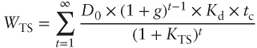
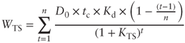
The discounted value of tax savings has been determined using ![]() in both scenarios.
in both scenarios.
9.7 DEBT PROFILE BEYOND THE PLAN HORIZON FORECAST
As mentioned, it is inevitable to use simplified assumptions for the cash flow trend beyond the plan horizon plan. In particular, we assume that:
- Perpetual cash flows are constant.
- Cash flows continue to grow in nominal terms.
- Cash flows continue to grow in real terms with articulated assumptions for the duration of real growth.
The credibility of the assumptions made obviously depends on the business category under consideration.
A similar reasoning can be followed for the cash flow profiles of the tax savings. Choices on tax shields can have a significant impact on the result of the valuation process.
9.8 THE VALUATION OF TAX ADVANTAGES: ALTERNATIVES
After having introduced an overview of the topic, this section discusses the different assumptions that experts consider in the estimation of WTS.
ASSUMPTION 3: WITH REAL GROWTH, THE DEBT PROFILE IS EQUAL TO THE DEBT LEVEL ASSUMED IN THE CASH FLOW (FCFO) PROJECTION
Under this assumption, debt conforms to the FCFO profile through different growth rates, which can be perpetual, differentiated according to the time period, or limited to a predefined period of time. Exhibit 9.13 graphically shows this concept.
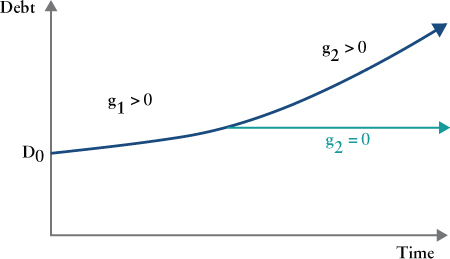
Exhibit 9.13 Debt pattern beyond the plan horizon forecast (assumption 3)
This assumption implies that the debt ratio stays constant over time. In particular, the growth in the value of the business (in nominal and real terms) corresponds to an equivalent increase in leverage.
It is important to remember that, whenever experts determine the terminal value using an aggregated method (i.e., by subtracting the growth rate from the WACC), they implicitly assume that the debt pattern mirrors one of the profiles shown in Exhibit 9.9.
The different relevant formulas are:
- Constant Growth:
from which:
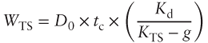
In the previous formulas, g expresses the total FCFO growth rate, which incorporates both the “real” growth rate and inflation dynamics.
In a temporary growth scenario, it is assumed that debt does not even increase in nominal terms once the growth period ends. This assumption can obviously be relaxed if needed.
- Limited Growth:
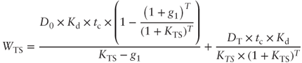
- Staged Growth:
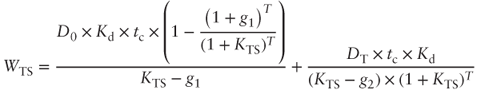
SCENARIO A:1
SCENARIO B:
where:
- n refers to the number of years of the repayment period
- c refers to the debt repayment rate when there is a lower debt floor D*:

Under the assumption that debt decreases to zero, it is possible to assume that first-year repayments are higher than end-of-period repayments. In this case, the analyst could use the discounted cash flow formula for a decreasing annuity:
where g refers to the decreasing debt rate over an infinite horizon.
Exhibit 9.15 shows debt profiles assuming a constant repayment equal to 10 percent of the initial debt amount (A) and assuming decreasing repayment instalments based on a 10 percent yearly rate (B).
It is interesting to highlight that the ![]() values in the two scenarios do not differ significantly as long as we consider normal debt repayment periods (5 to 10 years).
values in the two scenarios do not differ significantly as long as we consider normal debt repayment periods (5 to 10 years).
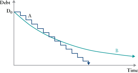
Exhibit 9.15 Debt profiles with constant repayment (A) and decreasing repayment (B)
Before discussing why we may want to relax the assumptions, we will verify their impact on tax benefits in Exhibit 9.16 under the valuation scenario described in section 9.6.
| Assumptions | KTS | WTS | g |
| 1) D constant | 21.6 | 0 | |
| 2) D constant in real terms | 27.5 | 1.50% | |
| 3) D increasing at FCFO growth rate | 36.3 | 3% | |
| 4) D decreasing at 10% | 9.2 | −10% |
It is necessary to point out that the analyst assumed a growth rate for the FCFO equal to 3 percent over an infinite time horizon in the estimation of the terminal value (this rate is the sum of the real growth rate and the inflation effect, estimated at 1.5 percent).
The alternative scenario assumes a lower debt limit of 60 million euros. ![]() is therefore computed based on a final year debt amount of 60 million euros.
is therefore computed based on a final year debt amount of 60 million euros.
![]() has been determined using
has been determined using ![]() in scenarios 1, 2, and 4. Two rates have instead been used in scenario 3:
in scenarios 1, 2, and 4. Two rates have instead been used in scenario 3: ![]() for the tax savings of the original debt amount;
for the tax savings of the original debt amount; ![]() for the incremental debt amount. If
for the incremental debt amount. If ![]() were the only rate used for all debt, we would have obtained a paradoxically lower
were the only rate used for all debt, we would have obtained a paradoxically lower ![]() than the one found in the no-growth scenario.
than the one found in the no-growth scenario.
9.9 GUIDELINES FOR CHOOSING DEBT PATTERNS FOR DETERMINING VALUATIONS
Exhibit 9.16 shows how different choices for the estimate of tax benefits can significantly influence results.
It is important to find the most appropriate and realistic debt pattern to use in the valuation process. Three major guidelines can help experts:
- Business cash flows: Businesses that generate cash flows are usually characterized by low leverage with the exception of abnormal growth periods. When a business generates cash, it is therefore reasonable to assume that debt decreases over, for example, a 10- to 20-year repayment plan.
- Book value of assets: Debt dynamics should be analyzed based on the book value of the company's assets since it would be dangerous to assume that the ratio between debt and assets could exceed acceptable limits.
- Value creation role assumed by leverage in a specific industry: It is useful to mention that leverage is considered an acceptable means of value creation for shareholders only in low risk (and relatively low but stable and visible profitability) industries. In these particular cases, it is then sensible to assume that the debt level increases over a long period or indefinitely.
Going back to one of the examples shown in this paragraph, the investment bank presented two different valuations of its tax benefits:
- In the first scenario, the analyst assumed debt to be repaid by t5. Tax shields are therefore not considered beyond the plan horizon.
- In the second scenario, the 60 million euro floor is used to determine the terminal value. During a discussion with management, it became clear it would be advisable to keep a certain degree of leverage, and to rebalance the financial structure possibly via extraordinary dividend payments and buybacks in favor of shareholders.
Exhibit 9.17 summarizes the valuation of tax shields in both scenarios.
Exhibit 9.17 Valuation of tax shields (mln /€)
Scenario a Scenario b  plan horizon
6.2 9.4  beyond the plan horizon
- 13.1  total
total6.2 22.5
It should be noted that the tax savings for the period beyond the business plan horizon have been discounted at the same ![]() used to determine
used to determine ![]() in the business plan period.
in the business plan period.
9.10 SYNTHETIC AND ANALYTICAL PROCEDURES VALUATION
The financial model application will be analyzed in this chapter based on the distinction between synthetic and analytic procedure. These procedures will be discussed in further details in the next two chapters.
9.10.1 Synthetic Procedure
The synthetic procedure allows us to follow an easy estimation process over long periods of time. It is called synthetic, as it is based on the assumption of some parameters staying constant. In practice, the synthetic procedure can be considered a good method only when some conditions hold. In particular, it is valid under these conditions:
- The company or project under valuation is in an equilibrium situation and it is reasonable to assume that no deviations from equilibrium will happen (steady state).
- The company is in an equilibrium situation and we can reasonably assume that some relationships between variables (investments, revenue growth, and margin growth) hold. This produces a growth cash flow model over a long enough period of time (steady growth).
For instance, going back to the cash flow model introduced in section 9.2 and considering the case of the hydroelectric company, a synthetic valuation formula would be suitable since the long-term cash flow is very similar to a growing perpetuity in nominal terms. This is due to the regulated price mechanism allowing for a full recovery of inflationary effects.
On the other hand, the cash flow profile of an energy company discussed in this chapter could represent a typical example of long-term growth based on the gradual expansion of the distribution channel.
9.10.2 Analytical Procedure
By contrast, the analytical procedure requires specific cash flow projections over the company's plan horizon. In practice, these processes should be used when the company is not at full capacity due to expansions or contractions, new investments, or new restructuring processes.
Considering the limited length of analytical projections (usually not beyond 10 years), these processes require the need to estimate the company value at the end of the forecasted period. This value is usually known as the terminal value (TV).
According to the company's characteristics, the TV can assume two formulations:
- The company value in equilibrium: In this case, the TV is determined following the formulas stemming from the synthetic procedure.
- The liquidation value when the company's life is limited: This scenario can be used, for instance, in the case considered in Exhibit 9.5, regarding the cash flow profiles of a company in the waste management industry. Otherwise, it can be used for companies that are under licensing when their licenses will not be renewed.
9.11 THE STANDARD PROCEDURE
Financial analysts generally use a standard process:
- Analytical projections usually cover a period of 3 to 5 years, which can extend up to 7 to 10 years in some industries. They are based on the business plan built by management, while a potential further extension of the plan is added to take specific characteristics of the business into account (e.g., cyclicality).
- The terminal value is estimated based on the normalized cash flow from the last year of explicit forecast, or of the last 2–3 years especially in case of cyclical industry/companies. Hence, the typical cash flow structure is the one shown in Exhibit 9.18.
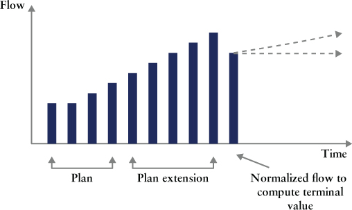
Exhibit 9.18 Typical cash flow projection in DCF valuations
As an alternative to the process we just discussed—also known as the pure DCF method—the TV is also often estimated through multiples of a sample of listed companies with similar characteristics to the firm under consideration. This alternative will later be presented in detail while analyzing the multiples valuation technique.
As already mentioned, the analytical process horizon is often longer than the standard plan horizon. This fact goes back to the previously highlighted issue of cash flows constituting only a small portion of the company value. Analysts dislike this problem and try to extend the forecast period to partially solve it. While analyzing a valuation outcome, discussions often arise about the portion of the company value, respectively represented by the terminal value and by cash flow projections.
In practice, the portion represented by the plan is relevant for two reasons:
- It is a risk measure. As a matter of fact, if the flows over the following five to seven years represent a small portion of the company value (e.g., around 20 percent), the estimated outcomes are quite sensitive to the assumptions made in the terminal value determination.
- If the cash flow plan represents a small portion of the company value, debt financing of an acquisition could be more complex.
Beside the aforementioned reasons, there are no other justifications why the TV should be above or below a specific percentage of the total estimated value.
____________________