1.1 The essence of an econometric model

An econometric model, in the form of a single stochastic equation, is a primary tool in econometrics. The subject of its description consists of a dependent variable Y with y_t observations, where t is the statistical observation’s number (t = 1, …, n) and n is the sample size. The dependent variable is economic in character and represents a specific economic category [1].¹

Explanatory variables marked as X₁, …, X_j, …, X_k, essentially, represent the factors causing variations of the dependent variable Y. Also, some statistical observations are assigned to each dependent variables: x_t1, representing the variable X₁, …, x_tj, representing the variable X_j, … as well as x_tk for the variable X_k.

The most general form of a model with a single stochastic equation can be written as follows:

(1.1)

with one more variable η_t, the random component. This random component gives the model its stochastic character and results from the following:

• The random nature of economic phenomena and processes.
• A conscious and purposeful resignation from complying with less important and statistically insignificant factors.
• Inaccuracies during observation and measurement of economic phenomena and processes.
• A lack of full precision in determining the equation’s analytical form.
• Round-ups in the course of numerical calculations during application of the procedures used to estimate the model’s parameters.

The most frequently used analytical form of the model is linear in character

(1.2)

A shorter version of this model can be written as follows:

(1.3)

In Equations 1.2 and 1.3, some structural parameters (α₁, …, α_j, …, α_k) appear, which are the measures of each explanatory variable’s impact on the dependent variable.² The parameter α₀ is called a constant term of the model and cannot always be interpreted in economic terms.

Product models, in literature also called multiplicative models, are the most commonly used ones among the nonlinear analytical forms of an econometric model. The first variant of this model is the power-law model, in the form

(1.4)

which concisely can be written as

(1.5)

The second multiplicative model is exponential in the form

(1.6)

Briefly, this model can be written as follows:

(1.7)

Finally, it is possible to use a type of a mixed multiplicative model, that is, a model of a power-exponential character. An exemplary power-exponential³ model can be written as follows:

(1.8)

Construction of an econometric model occurs in the following five subsequent stages:

1. specification of the model,
2. identification of the model,
3. estimation of the model’s parameters,
4. verification of the model,
5. application of the model

During the specification stage, the purpose and the scope of the test are established as well as a set of the model’s variables: a dependent variable and explanatory variables. A measurement method for those variables is then indicated. All statistical data necessary for the test, such as the time series or cross-sectional data,⁴ have to be collected. Finally, it is necessary to formulate the model’s hypothesis in an adequate analytical form of an equation(s).⁵ Such a specification results in a hypothetical (theoretical) econometric model.

Model identification becomes necessary in case of a model composed of many stochastic equations. Mathematical accuracy of the model’s structure, which is discussed in Chapter 2, needs to be settled.

Estimation of the model’s parameters involves a selection of an estimator, which is appropriate for the hypothetical econometric model.⁶ An estimator is used for numerical calculations. Using all available statistical information for calculations, the model’s structural parameters and its stochastic structure’s parameters are estimated.

Model verification involves checking its statistical quality and examining the empirical model’s economic logic. Analysis of statistical quality requires using specialized goodness measures⁷ and various statistical tests.

Model application is using the empirical model in accordance with its purpose and its constructional aim. This can serve as a support in economic decision-making. Another line of the model’s use is simulation. The models based on time series are most frequently used in forecasting of economic phenomena and processes.

1.2 Specification of an econometric model

From an economic viewpoint, econometric model’s specification is the key to its proper construction. Any deficiencies in specification can result innumerous defects of that model.

Defining an economic system and its components is fundamental in specification. The components of an economic system are represented by variables: the dependent and the explanatory ones. In the model represented by a dependent variable, many of those components can be defined and measured in several ways. The dependent variable should be defined and explained in such way that it is equivalent⁸ to the economic object or its feature.

For instance, an economic category such as production can be represented by a number of variables. These could, for example, be the value of ready-made production accordingly to its manufacturing costs, the value of a finished production in sale prices, net sales income, gross sales income,⁹ or the amount of the cash inflows from the sales of goods and services. In a given model, depending on the study’s aim, production can be represented by a variable appropriate for a particular case.

Consideration of factors that may influence a given dependent variable (either by stimulating or by impeding it) leads to specification of potential explanatory variables in the model. Influence of these explanatory variables on the dependent variable will be a subject to verification through the empirical model.

After both types of variables, the dependent and the explanatory ones, are determined, it is imperative to collect all statistical data necessary for their analysis. The number of statistical observations done on each potential variable of the model is important and must visibly exceed the number of explanatory variables. A condition of the so-called large statistical sample ought to be met. Lack of essential statistical information, its poor quality, or a significant number of gaps in the statistical material all can preclude the conduction of an econometric investigation based on the model. Slight gaps in statistical data can be complemented by using some statistical techniques (i.e., interpolation and extrapolation). Collection of valid statistical data on the model’s potential defined variables completes the variable specification stage, which allows transition onto the equation specification stage.

Specification of equations consists in determining the number of equations within the model and a choice of an analytical form for each of those equations. Econometrics offers a vast arsenal of possible analytical forms. However, type 1.2 linear equations as well as type 1.4 and 1.6 product equations are most frequently used. The model’s specification stage ends with a choice of the equation’s (equation) analytical form. A hypothetical (theoretical) econometric model is its result.

1.3 Estimation of an econometric model’s parameters

Estimation of the model’s structural parameters and its stochastic structure parameters requires having a theoretical model as well as all necessary data collected on each variable of that model. First, an estimator, that is, a function estimating the model’s parameters, must be selected. An estimator holds the following properties:

1. Unbiasedness – let be an estimator of the parameter θ, based on the set of observations {y_i} as . If equality occurs, then is called the unbiased estimator of the parameter θ. When , the estimator is negatively biased; but if , the estimator is positively biased.
2. Consistency – if the estimator converges in probability to θ, and when , then is the consistent estimator of the parameter θ; , according to probability, seeks to be θ, when
   (1.9)
   It is worth noting that for appropriately large n-values, the consistent estimator is always unbiased. However, the opposite is not always true, since an unbiased estimator does not have to be consistent.
3. Efficiency – let , j = 1, 2 be the two estimators of the parameter that are based on the observation set {y_es}. Efficiency of the estimator , in relation to the estimator _, can be defined as the quotient of
   (1.10)
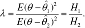
   In this case, we did not limit ourselves to a class of unbiased estimators; thereby H₁ and H₂ do not need to be the error variances. If we limit ourselves to the unbiased estimators and , then H₁ and H₂ are the variances. The estimator is called an effective estimator of the parameter θ, if H₂ ≥ H₁ occurs for each of the other unbiased . In other words, no other unbiased estimator has a variation lower than . It is worth to mention a volatility characteristic that is alternative to a statistical deviation – the estimator’s precision (κ), defined as , where σ is the standard deviation. An estimator of a lower variance, that is, of a lower standard deviation, 87 + 910 is characterized by a higher precision. Thus, a statement can be made that an estimator of a higher efficiency is a more precise estimator.
4. Sufficiency – an estimator is sufficient when it contains all information included in an observation set of the parameter being assessed. Let us suppose that y₁, y₂, …, y_n is an observation sequence in a sample randomly selected from a population having the density function f(y, θ). If is such an estimator of the parameter θ that the conditional expected value does not depend on θ, then is a sufficient estimator.

The ordinary least squares method (OLS), developed by Carl F. Gauss, is the first general estimation method having many mutations. It consists in such selection of an estimator, , so that the sum of squared differences between the observations y_i and their corresponding values of the function is minimal

(1.11)

The OLS method is widely applied in practice, although it requires meeting such criteria, which give the OLS estimator some essential statistical characteristics. Let us consider a linear model

(1.12)

where

and

(1.13)

where

In model 1.12, X is the matrix of observations on the model’s explanatory variables, Y is the vector of an observation on the dependent variable, η is the vector of the random components, α is the vector of the structural parameters, n is the number of statistical observations, and k is the number of explanatory variables. Hypothetical model 1.12 was assigned an empirical model (1.13), in which there are two new vectors:  – an estimator of the vector α, and u – a residue vector. Having the estimator , theoretical values of the dependent variable can be assigned

(1.14)

where a vector of the dependent variable’s theoretical values, which were calculated using the model 1.14, emerges:

The conditions of the OLS method application can be described as follows:

1. An econometric model must be linear in form, such as Equation 1.2. If a nonlinear model can be transformed into a linear one, then the OLS method is allowed. For example, the power-law model 1.4 and the exponential model 1.6 both can be transformed into linear forms using a logarithm of both sides.
2. Mathematical expectation of the random component should be equal to zero:
   (1.15)
3. The random component’s variation (σ²) should be constant and finite, such as
   (1.16)
4. The sequence of matrices of observations on explanatory variables, represented by X, is equal to the number of the model’s structural parameters (k + 1):
   (1.17)
   This means that the n number of statistical observations is higher than the number of the model’s structural parameters. In other words, the model has a positive degree of freedom. Moreover, none of the explanatory variables is a linear combination of another variable of the same type.
5. Explanatory variables should be correlated with the random component. This can be written as
   (1.18)
6. The random component should be devoid of autocorrelation, such as
   (1.19)
   where E(ηη^T) is the matrix of random components’ variances and covariances. Zero elements outside the main diagonal indicate that the covariances of the random components for their various pairs are equal to zero, that is
   (1.20)

The second group of econometric model’s parameters is formed by the stochastic structure’s parameters. They describe a distribution of the random component η. It is usually assumed that distribution of the econometric model’s random component is normal [N(0, σ²)]. The assumption of a normal distribution of the random component η, which has a zero expected value, can be interpreted as follows:

1. positive and negative random deviations compensate each other;
2. the number of positive random deviations is close to the number of negative ones;
3. it can be expected that most random deviations will slightly differ from zero, and over 99.7% of all random deviations should fall within the spectrum of  ±3SD. A standard deviation of the random component (σ) provides information on how much, in plus or in minus, the standard observations of a dependent variable (y_t) deviate from the function . The lower the σ value, the smaller the random part of the explanatory variable.

Using the criterion written as Equation 1.11, the OLS estimator for vector α can be written as follows:

(1.21)

where X^T is a transposition of matrix of observations on the explanatory variables X. The random component’s variance (σ²) needs to be estimated as well. It can be shown that a residue variance (Su²) is the unbiased estimator of a variance of the model’s random component, and it can be calculated using the following equation:

(1.22)

where ŷ_t represents the theoretical values of the dependable variable, which are calculated using the empirical model, while u_t represents the model’s residuals. Alternatively, Equation 1.22 can be written as a matrix

(1.23)

where u is the residual vector, defined in relation to Equation 1.13.

The Aitken’s method, which is a generalized OLS method, also called a generalized method of the least squares,¹⁰ is another method used for estimation of the model’s parameters.

An Aitken estimator () can have the following form:

(1.24)

where a weight matrix Ω appears in the form of

(1.25)

where ω₁, …, ω_t, …, ω_n are the weights, which include the volatility of the random component’s variance for various observations. What is more, when ω₁ = = ω_t = = ω_n = 1, matrix Ω = I; in other words, it becomes a unit matrix of the n degree. As such, the Aitken estimator becomes equipotent to the OLS estimator.

In the Aitken’s method, an estimator of the random component’s variation is given by the following formula:

(1.26)

1.4 Verification of the model

Statistical verification of the model involves using multiple measures which, first and foremost, characterize the random component’s role in that model. The first of such measures is a residual variance, discussed in the previous subsection. It does not have any economic interpretation. The square root of the residual variance

(1.27)

is called standard residual error. Su is expressed in the same measurement unit as the dependent variable y_t. It provides information on how much, on average, during an n number of statistical observations, the theoretical values of the dependent variable ŷ_t, which are calculated using an empirical model, are different from the actual (observed) values of that variable (y_t).

The second-general measure of a model’s accuracy provides information on the relative role of the random component. The convergence factor ϕ² is calculated using the following formula:

(1.28)

where represents the average arithmetic value of an observation on the dependable variable. It measures the relative share of the model’s random fluctuations in the total variability of the dependent variable . The smaller the share of random variability in the total volatility of the dependable variable, the better the empirical model. The convergence factor is a normalized number and meets the condition of . By this criterion, the closer to zero the ϕ² is, the better the empirical model. Expression 100 ϕ² (%) provides information on what percentage of the total variation of the dependable variable y_t is random.

A square root of a multiple-correlation coefficient, also called a coefficient of determination, represented by R², is an alternative measure of the model’s accuracy. This measure indicates which part of the dependable variable’s total fluctuation is generated by explanatory variables of the empirical model.

A coefficient of determination is calculated as follows:

(1.29)

The expression 100 R² provides information on what percentage of the dependable variable’s total fluctuation results from the impact of the set of the empirical model’s explanatory variables. Therefore, the closer to unity the coefficient R² is, the better the model.

The next issue is to examine the random component’s autocorrelation.¹¹ Lack of this autocorrelation means that we are dealing with the so-called pure random component.

The presence of the random component’s autocorrelation means that the random component creates an autoregressive process, in the form of

(1.30)

where ε_t is the pure random component. The autocorrelation coefficients of the random component ρ₁, ρ₂, …, ρ_n−1 with a value different from zero, indicate this autocorrelation’s occurrence. The Durbin–Watson test is a tool used to test the random component’s autocorrelation of the first order.¹² It verifies the null hypothesis, which assumes ρ₁ equal to zero and is written as H₀:ρ₁ = 0. An alternative hypothesis assumes that ρ₁ is positive, and so H₁:ρ₁ > 0.

The Durbin–Watson (DW) statistic tests the null hypothesis and is calculated by the following formula:

(1.31)

where u_t marks the residuals from the t-period (t = 1, …, n), while u_t−1 represents residuals delayed by 1 period. In case of a large sample, the DW statistic falls within 0 ≤ DW ≤ 2, where ρ₁ is positive. Thus, if the DW statistic > 2, the alternative hypothesis ought to be changed to assume occurrence of the random component’s negative autocorrelation; in other words, H₁: ρ₁ < 0. In such cases, a corrected Durbin–Watson statistic should be calculated using the following formula:

(1.32)

The estimated DW (or DW*) values are compared with the test’s critical values: a lower d_l value and an upper d_u value, both taken from Durbin–Watson¹³ tables, on an appropriate γ level of significance.

If, based on the above introduced tools of statistical verification, the empirical model can be considered acceptable, the statistical significance of explanatory variables should be studied as next. Having the empirical econometric model

(1.33)

in which a_j (j = 0, 1, …, k) represents assessments of the structural parameters and u_t represents the residuals. The empirical model, alternatively, can be written as follows:

(1.34)

where ŷ_t represents a theoretical value of the dependable variable in a t (t = 1, …, n) period.

Equations 1.33 and 1.34 differ by their residuals (y_t − ŷ_t =  u_t). Each structural parameter’s estimate (a_j) is characterized by its corresponding average estimation error (j = 0,1, …, k), which is a square root of the jth variance of the structural parameter’s estimate and provides information on that estimate’s accuracy. It is, therefore, necessary to assign estimation variances of the model’s structural parameters. The matrix of the structural parameters’ variations and their covariations [D²(a)] should be assessed, using the following formula:

(1.35)

where Su² is the residual variance provided by Equation 1.22 and (X^TX)⁻¹ is an inverse of the so-called Hess matrix occurring in Equation 1.21. Diagonal elements of the matrix D²(a) are the variances of the structural parameters’ respective estimates, that is

(1.36)

Using the average errors of the structural parameters’ estimations, the empirical model can be written as follows:

(1.37)

where the average estimation errors are written in parenthesis under the structural parameters’ estimates.

Having the model 1.37, a test on explanatory variables’ statistical significance can be conducted. We pose the null hypothesis H₀:α_j = 0 (j = 1, …, k), which means that the jth structural parameter equals zero. In an economic sense, this is a hypothesis about insignificance of the model’s jth explanatory variable. An alternative hypothesis H₁:α_j ≠ 0 assumes that the jth structural parameter is different from zero, which marks statistical significance of the jth explanatory variable.

An empirical statistic of a t-Student serves as a null hypothesis test, provided by the equation¹⁴

(1.38)

where the absolute value of the jth structural parameter’s estimate is in the numerator, while its average estimation error is in the denominator.

The critical value t_γ;n−k−1 should be read from the tables of a t-Student distribution’s critical values. A reasonable level of significance¹⁵ γ is selected arbitrarily. The reading is done while having an −k − 1 number of the degrees of freedom. Comparing the empirical statistic t_j (j = 1, …, k) with the critical value t_γ;n−k−1, we infer the significance of the jth variable. If there is an inequality t_j ≤ t_γ;n-k1, then there is no reason to reject the null hypothesis. Basically, this forces a removal of that variable from the empirical model, then re-estimation of its parameters and verification of the respecified model. When t_j > t_γ;n−k−1, the hull hypothesis is rejected in favor of an alternative hypothesis and we infer a statistically significant impact of the jth explanatory variable on the dependent variable. Statistically insignificant variables are eliminated from the model. In a given iteration, only one irrelevant variable – the one for which the statistic t_j is the smallest – ought to be eliminated. Such recalculation and reverification of the model is done until all empirical variables of the model are statistically relevant on a reasonable level of significance. By doing so, we get an acceptable empirical econometric model.¹⁶ This empirical model is often written as follows:

(1.39)

where the empirical t-Student statistics are under the structural parameters’ estimations. With such a model, we make its economic evaluation, which involves assessing the compatibility of modeling results with economic theory and the logic of economic practice.

1.5 Multiplicative econometric models

Multiplicative models¹⁷ – after linear models – belong to a category of nonlinear models most frequently used in economic research. Both groups of multiplicative models can be converted into linear ones. Let us consider a power-law model 1.4

A logarithm on both sides of the above equation is obtained as follows:

(1.40)

Substituting , , , for j = 1, …, k; model 1.40 can be written as

(1.41)

Equation 1.41 is linear in character due to its parameters. The structural parameters thus can be assessed using the OLS method.

A similar transformation can be done using the exponential model 1.6

Applying a logarithm on both sides to the above equation, we get its following converted form:

(1.42)

Consecutively substituting , , j = 0,1, …, k, the model 1.41 can be written in a linear version

(1.43)

The parameters of Equation 1.43 can be assessed using the OLS method. Using the formula 1.21, we get the following matrices of observations on the dependable variables

Equation 1.21 will take the form

(1.44)

where

Parameters of the equation type 1.43 can also be assessed using the OLS method, while the estimator takes on the following form:

(1.45)

where Y^* has the same form as in the previous case 1.41 and the vector has the form

Let us suppose that the parameters of the power-exponential model in the form of Equation 1.8 were assessed:

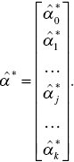
The vector of the structural parameters’ estimates was obtained in the following form:

Thus, the estimates of the structural parameters are known

We note that the estimates of parameters are given in the form of logarithms. It is therefore necessary to perform the following calculations:

The power-exponential empirical model, thus, has the form

(1.46)

In the power-law model, all estimates of the structural parameters are obtained directly (except the a₀ estimate), whereas in the exponential model, additional calculations are always necessary to obtain the estimates a_j (j = 0,1, …, k).

1.6 The limited endogenous variables

The dependent variable of an econometric model should be characterized by a relatively large area of volatility. It should also not be limited. What it means is that it should have neither a lower nor an upper limit. Meanwhile, sometimes the model has variables performing the role of dependable ones with observations , which can have bilateral restrictions. Their specificity is that of having a lower and an upper limit, namely as in

(1.47)

where y_min means the lowest possible observation value of the considered variable, while y_max is the highest possible observation value for this dependable variable.

Let us suppose that the limited variable will be described using a linear model

Figure 1.1 shows a linear econometric model for the limited dependable variable. The consequences of possible extrapolation beyond the statistical observation area are noted. Such an attempt of extrapolation may lead the extrapolated values to fall outside the area of limited variable’s volatility, which is contrary with logic. For instance, the structure indicator, which satisfies the inequality , can be the limited variable. An attempt to extrapolate the variable in the form of a structure indicator can lead the extrapolated values to be less than 0%, or greater than 100%.

Application of one out of many possible transformations of the limited dependent variable could be a possible solution here. The first of such transformations is a basic transformation of the limited variable, given by the following formula:

(1.48)

where the symbols are identical to those in formula 1.46, while on the contrary, represents a basic transformation of the both-sides limited variable . A basic transformation of the limited dependent variable converts it into a variable, which takes its value from the range . A variable in the form of is unlimited in its non-negative values. Still, its lower limit is on the 0 level; thus it has the characteristics of many economic variables that reach non-negative values.

Figure 1.2 shows a basic transformation of the variable , wherein the minimum value of the dependent variable is 0, that is, y_min = 0. It does not, however, change the generality of the idea shown in this figure.

Next important transformation of a both-sides limited variable is the logit transformation, the idea of which is shown in Figure 1.3 and is given by the following formula:

(1.49)

A logit transformation of the limited variable is thus a logarithm of the basic transformation. It converts the variable into a both-sides limited variable. In fact, we can see that the variable in a logit form fulfills the inequality . Thus, application of linear models, such as

(1.50)

or

(1.51)

eliminates the risk associated with extrapolation of the dependent variable beyond the statistical observation area.¹⁸

Estimation of the parameters from a model with a limited dependable variable can be done using the classic least squares method, with application of the procedure provided by Equations 1.21–1.23. Goldberger suggests¹⁹ that in such a case, the Aitken estimator provided by Equation 1.24 is more accurate. As such, a question emerges, how to estimate the components of the matrix Ω provided by Equation 1.25.

In this case, a double-step procedure is required. In the first step, the OLS method should be used to estimate the parameters of the model with an endogenous dummy variable. After theoretical values from a 1.34-type empirical equation are calculated, weights for each observation can be assigned, using the following calculation:

(1.52)

A result, an empirical matrix can be constructed in the following form:

(1.53)

In practice, negative values of the weights w_t can appear. Therefore, it is better to use weight modules calculated using formula 1.52. Matrix then will take the following form:

(1.54)

Aitken estimator for the dummy explanatory variable will then have the following form:

(1.55)

Matrix will have the following structure:

or

(1.56)

Estimator 1.55 provides more effective (precise) parameter assessments of the model with a dummy explanatory variable, in comparison with the OLS estimator.

1.7 Econometric forecasting

1.7.3 Forecasts based on single-equation models

Let us suppose that the following single-equation linear econometric model is used in a prediction

where η_t is the pure random component of a zero expected value. Depending on the applied estimator of the structural parameters’ vector, we can get various predictors.²⁶ If the parameters of the above model were estimated using the least squares method (OLS), the predictor used in the forecast will be according to the OLS method and will have the following form:

(1.57)

where are the estimates of parameters α₀, α₁, …, α_j, …, α_k, calculated using the OLS method. The symbol T represents the forecasted period, wherein T = n + 1, n + 2,…, n + τ. For example, using an estimator of a generalized OLS method (Aitken’s method), we will get a predictor according with the Aitken’s method, and so on. The predictor equation 1.57 can be written in a matrix form as

(1.58)

where is the vector of explanatory variables in the forecasted period T, while the transposed vector of the structural parameters’ estimations has the following form:

A prediction variation for the predictor equation 1.57, thereby for Equation 1.58, is assigned using the formula

(1.59)

where represents a prediction variation of the forecasted variables in the T period, X_T is the vector of explanatory variables’ values in the forecasted period T, σ² – a variation of the model’s random component.²⁷ Equation 1.59 alternatively can be written as

(1.60)

where the matrix of the model’s structural parameters’ variance and covariance , calculated using the OLS method, appears.

It can easily be shown that the following inequality occurs:

(1.61)

This means that prediction accuracy cannot be greater than the accuracy of the model used in the empirical model’s prediction.

Square root of the prediction variance is the average prediction error, that is

(1.62)

The average prediction error is expressed in the units of the forecasted variable Y_T. It allows assessment of prediction accuracy in a period T. The requirement appropriate forecast accuracy is defined by its user, setting the prediction’s limiting error V_G. If the following inequality occurs:

(1.63)

then the forecast is admissible, since it fulfills the requirement of the precision desired by the user. In case of the following:

(1.64)

the forecast is inadmissible, since it is not accurate enough for the user’s needs.

Often, it is difficult for the user to determine the value of the average prediction error V_G for each of the forecasted variables. It is easier to determine the relative limiting error of prediction expressed as a percentage of the forecast’s value. In that case, a prediction accuracy measure is used, such as the relative limiting error calculated using the following formula:

(1.65)

Comparison of the relative average error of prediction with the relative limiting error of prediction allows appropriate decision-making. In case of the following:

(1.66)

the forecast is deemed admissible; in terms of the user’s needs, it is sufficiently accurate. However, in case the following inequality occurs:

(1.67)

the forecast is inadmissible, since from the user’s perspective, it is not precise enough.²⁸

1.7.4 Analysis of econometric forecasts’ precision

Besides using the measures of prediction accuracy, which allow its ex ante type of estimation, it is necessary to observe and to register the realizations of the forecasted variable y_T. Knowledge of the forecasted variable’s realization allows its comparison with the forecast. This enables testing the expired forecast,²⁹ using forecast accuracy measures of the ex post type.

The difference between the forecasted variable’s realization in the T (y_T) period and the (y_Tp) forecast, marked as ω_T, will be called the forecast error; in other words

(1.68)

Even one forecast error observation ω_T can cause a necessity of interference into the forecast results. A grossly inaccurate forecast may emerge. This happens when a forecast error exceeds an average forecast error (). Such a case may signify a future set of inaccurate forecasts, often with homonymous signs of forecast errors.

Emergence of a set of forecast errors with the same sign means that a set of underestimated or overestimated forecasts has formed. A sequence of overestimated forecasts appears, when , in few consecutive forecasted periods. A sequence of underestimated forecasts appears, when inequality occurs in at least three periods. A reaction to such an occurrence should consist in predictor’s correction, which involves a change of the set of explanatory variables in the empirical model, a change of the equation’s analytical form, and supplementation of modeling information with the data resultant from realization of a forecasted variable.³⁰

Valuable information on the accuracy of the forecasted prognoses against the forecasted variable’s realization is provided by the average forecast error δ_υ, which can be calculated using the following formula:

(1.69)

where T (T = t₀ + 1, …, t₀ + υ) denotes the forecasted period’s number and υ represents the amount of expired forecasts. The average forecast error provides information on how much (on average) the forecasted variable’s realizations differ from the earlier estimated forecasts. The meter 1.69, of course, can be calculated only after the forecasted variable’s realization is obtained, that is, while having the υ string of expired variables. The smaller the value of δ_υ, the more accurate the expired forecasts.

As proposed by A. Gadd and H. Wold, Janus coefficient J is an interesting measure of forecast accuracy. It is calculated using the following formula:

(1.70)

where {ŷ_t} is the sequence of endogenous variable’s theoretical values in the sample, on the basis of which empirical model’s parameter estimation was conducted, while n is the number of observations in the statistical sample. All other signs are the same as in formula 1.69. The Janus coefficient, thus, is the quotient of an average squared forecasting error and the average squared equation residuals in the sample. An econometric model can be used as a predictor in the prediction process, as long as the J coefficient is equal to unity or only slightly exceeds 1. If, however, J significantly exceeds 1, predictor correction should be applied, using the newest statistical data.