
6
Econometric model in the analysis of an enterprise’s labor resources
6.1 A study of a mechanism of the demand for labor
In an enterprise, the mechanism of the demand for labor can be described using equations, in which employment functions as the explanatory variable. Familiarity with the mechanism of the employment’s volatility in an enterprise allows recognition of employment stimulators, inhibitors, as well as some neutral1 factors. Small enterprises play a particular role in the study on labor demand, since in those companies lays the biggest potential to generate job positions and consequently, the growth of the domestic product. Also, knowledge about labor demand in large- and medium-sized enterprises can foster creation of the regulators of the processes, both within the company as well as in the so-called outside world. In this chapter, various approaches to econometric modeling of employment in as small-sized enterprise will be presented. Similar procedures can be used to analyze employment in medium- and large-sized enterprises.
A relative ease of establishing and developing small-sized enterprises – within certain limits – provides an opportunity of fast economic growth, thereby reducing the number of the unemployed. Therefore, this group of companies constitutes the biggest opportunity for every economic system. Development of small businesses, thus, should belong to the strategic goals defining our future. Therefore, it is necessary to quickly eliminate the barriers hindering both the creation as well as operation of this group of companies. It is urgently necessary to remove the causes of the decreasing labor demand of small companies. In turn, in small-sized companies, it is necessary to implement new technologies of diagnosing the situation on important fields of their activity, which will contribute to rationalization of the decisions.
In this chapter, we will present the consequences of the changes in various external and internal factors, including an increase in a small-sized enterprise’s tax burdens, on shaping the size of employment. Internal factors result from the actions of the company’s owner, his/her autonomous decisions about the production and its structure, the markets, investments, and the company’s organizational structure. External conditions result from actions of the state, the local government, or the competitive environment, as well as from the condition and the dynamics of the job market.
Development of a small-sized enterprise, in the first phase, generally entails an increase in employment volumes. An increase in production requires greater production potential, embodied in its factors. Job resources of a company result from a dynamic economic calculation. This calculation ultimately settles the company’s employment trends. The components being considered are both the company’s internal elements and external ones. The external and the internal factors sometimes penetrate each other, forming various hybrids.
The products as well as the technology used for its manufacture in reference to the entrepreneur’s resources, both decide about the proportions of the production factors implemented by him/her. The considered costs of each of those factors are generally formed outside the enterprise, only partially being formed directly in the company. A group of institutional factors, which are regulated by the state, plays a large part in creating the demand for labor. These include various solutions contained in law, especially in the labor law, such as, for example:
- working time,
- the minimum wage,
- the burdens of various costs connected with hiring and employee,
- the length and variety of vacation time,
- the conditions related to a conclusion and termination of employment contracts, and
- the benefits associated with absenteeism at work and many others.
Institutional solutions form many of the variables in the enterprise, according to a principle of savings. Thus, the impacts of external factors on the volumes of employment in reality are transferred onto the variables, on which it is possible to conduct statistical observations inside the enterprise. The results of this impact, ultimately, are embodied in the company’s labor resources.
Figures 6.1 and 6.2 demonstrate the changes in the employment volume in the company REX,2 respectively, monthly and quarterly in the years 1996–2006. Both graphs reveal a significant increase in employment since 1998.3 The process of reductions in the company’s labor resources started in 1999. Increases in the sales income were obtained through intensification of business activity.

Figure 6.1 The monthly dynamics of employment in the company REX, in the period from January 1996 to December 2006.
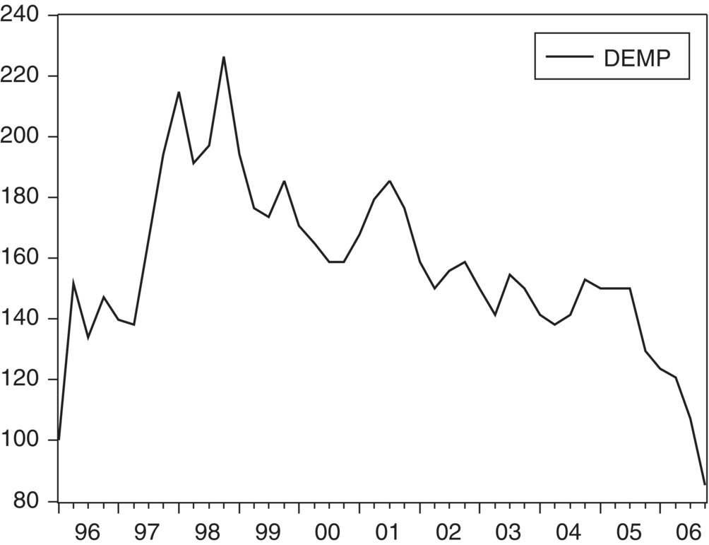
Figure 6.2 The quarterly dynamics of the company REX’s employment in the period from the first trimester of 1996 to the fourth trimester of 2006.
During the period being considered, the cost of labor in the enterprise had significantly increased. The average net wages increased both monthly as well as quarterly, which is illustrated by Figures 6.3 and 6.4. Similar trends occurred in the cost of labor per one employee, which is demonstrated by Figure 6.5. The requirements of the competition on the market, especially of the price competition, forced the company to adjust the costs to the standards of their competitors. It was necessary to take the measures increasing labor efficiency. This resulted in a decrease in the unit cost of the products, or at least in stopping its increase.

Figure 6.3 The monthly changes of the average net wage in the company REX, in the years 1996–2006.

Figure 6.4 The monthly changes in the technical devices into machinery and equipment, in the years 1996–2006.

Figure 6.5 The monthly changes of the VAT tax, in PLN per one employee, in the years 1996–2006.
Consequently, some investments4 appeared which substituted human labor with technology, embodied by machinery and equipment. An increase in the technical devices’ level through machinery and equipment (Figure 6.4) caused an increase in the labor efficiency. Simultaneously, during the period being considered, a process of a decline in an economic efficiency of the wages occurred. Changes in the value of the wage efficiency of the net sales meant that out of each thousand PLN of wages in the enterprise, lower and lower net sales income was obtained. In annual terms, during the initial period, out of a 1000 PLN of the net wages, over 12,000 PLN of the sales income was obtained.
Since 1997, the labor efficiency measured as such, which in 2006 had reached the level of just above 4700 PLN of net sales income per 1000 PLN of the net wages, was systematically declining. The curve of this variable’s trend is slowly decreasing in character. Maintenance of the market position required keeping up with the competitors’ prices. After 2000 begun the process of decreasing prices in this industry, which was forced by a major import of cheap finished products from Asia and especially from China.
In the past period, the burden of the business’ fiscal expenses had been increasing. In addition to the part contained within the labor costs, the burden of the tax on goods and services (Figure 6.5) had been increasing as well. In the initial period (1996–1998), the annual value of VAT, calculated per one employee, oscillated around 8000 PLN. In the subsequent years, it had increased systematically, exceeding the amount of 14000 per one employee in 2006.
As a result, a further decline in the profitability of the enterprises forced them to seek savings. Significant savings of expenses were possible in their largest areas. The costs of labor were in this group. Stopping an excessive increase in the labor costs had induced a process of employment volume reduction in the enterprise.
The volume of the enterprise’s employment resulted from an impact of various internal and external factors. At the same time, a view can be expressed that the internal and the external factors penetrated each other. As a result of that, hybrid variables formed, which embodied the forces inside the company as well as outside it.
A modeling study based on monthly data, from January 1996 until December 2006, was conducted. The dependable variable is expressed by a dynamics index of a constant base.5 The variable DEMP here represents the dynamics index of employment (in percentage points). Autoregressions of the 1st and the 12th order6 were considered in the model. The following explanatory simultaneous variables along with their delays were also considered:
- VATW – the monthly value of the tax on goods and services in PLN per one employee,
- TAM – the technical devices in machinery and equipment, monthly in thousands PLN per one employee.
Each of the explanatory variables was considered with an adequate time-delay from 1 to 12 months.7 In the initial hypothetical version of the model, the dummy seasonal variables and the time variable were also considered. They turned out to be statistically insignificant, similarly to the time-delayed variables. As a result, the following empirical8 model was obtained, which is presented in Table 6.1.
Table 6.1 An empirical monthly econometric model describing the changes in the company REX’s employment dynamics.
| Dependent variable: DEMP | ||||
| Method: least squares | ||||
| Date: 03/25/2014, time: 12:34 | ||||
| Sample(adjusted): 1996:12 2006:12 | ||||
| Included observations: 121 after adjusting endpoints | ||||
| Variable | Coefficient | Standard error | t-Statistic | Probability |
| C | 40.64787 | 8.664094 | 4.691531 | 0.0000 |
| DEMP(−1) | 0.953657 | 0.052992 | 17.99614 | 0.0000 |
| DEMP(−2) | −0.223040 | 0.064047 | −3.482414 | 0.0007 |
| DEMP(−3) | 0.127650 | 0.048642 | 2.624245 | 0.0099 |
| DEMP(−10) | −0.101014 | 0.043173 | −2.339768 | 0.0211 |
| DEMP(−11) | 0.090973 | 0.040679 | 2.236343 | 0.0273 |
| VATW(−6) | −0.004254 | 0.001277 | −3.332787 | 0.0012 |
| TAM | −7.230007 | 0.438921 | −16.47223 | 0.0000 |
| TAM(−1) | 6.833970 | 0.478718 | 14.27555 | 0.0000 |
| R-squared | 0.964636 | Mean dependent var | 180.1653 | |
| Adjusted R-squared | 0.962110 | S.D. dependent var | 32.14507 | |
| S.E. of regression | 6.257127 | Akaike info criterion | 6.576788 | |
| Sum squared resid | 4384.984 | Schwarz criterion | 6.784739 | |
| Log likelihood | −388.8957 | F-statistic | 381.8860 | |
| Durbin–Watson stat | 1.793400 | Prob (F-statistic) | 0.000000 | |
The model in Table 6.1 describes the mechanism of the employment’s9 volatility with high accuracy. The explanatory variables explain 96.8% of the total employment volatility in the enterprise. The actual values of the dynamics indexes differ from the theoretical values calculated on the basis of the model 6.1, on average, by 6.26% points, which is 3.47% of this index’s average monthly value in the years 1996–2006. In the model, there is no autocorrelation of the random component (Figure 6.6).

Figure 6.6 The actual and the theoretical volumes of the labor dynamics indexes (of the model from Table 6.1) and the model’s11 residuals.
Autoregressive10 dependencies play the most important role in description of the employment’s volatility mechanism. Autoregressions of the 1st, 2nd, 3rd, 10th, and 11th order turn out to be statistically significant. At the same time, an impact of the employment delayed by 2 and 10 months signifies the corrections of the signs in the employment changes with those period lengths.
The amount of the tax on goods and services per one employee plays an important role in the formation of the employment volume. The variable VATW(−6) significantly influences the dependable variable. The sum of the signs along those variables is negative (it is equal to −0.003). This means that an increase in the burden of the tax on goods and services, calculated per one employee, results in a decline in employment after the period of 12 months. An increase of that tax has price-making significance; it results in an increase in the prices. After 1 May 2004, a significant increase in the VAT burden is observed, since over 99% of the goods were covered by the 22% tax rate, while earlier on only about half of the company’s goods were under this tax rate.
The current and the delayed by 1 month technical devices in machinery and equipment have significant influence on the size of employment. A negative value of the structural coefficient’s assessment is higher, as far as the module and the openness of the positive parameter’s assessment are concerned. This means that on the balance sheet, expansion of the technical devices into machinery and equipment induces a decline in the company’s employment sizes.
Extracting “clean” internal and external factors, which form the enterprise’s employment, is possible only on a sufficiently high level of abstraction. Empirical assignment of adequate variables to one of the abovementioned groups of employment factors does not seem to be possible.
The variables that possibly can be included in the study, stimulating or hindering the size and the structure of employment, essentially have a hybrid nature. They form a kind of a “mix” of various types of factors. Thus, an empirical definition of the variables representing a particular external or internal factor of employment’s volatility seems to be an illusion.
The econometric model of employment in a small-sized enterprise presented in this work contains explanatory variables of varied nature. Each of those statistically significant variables is a condensate of many employment factors. Only those possibilities – in fact, limited – of empirical studies on employment factors in a small-sized enterprise exist.
The next econometric model of employment in the enterprise is designed to assess the impact that the burden of the tax on goods and services has on companies. This is due to permanent changes within the taxation legislature. Instability of the institutional system is most burdensome for companies. As a result of this situation, it is difficult to conduct long-term policies within the company. This results in an intensified caution when deciding about increasing resources, especially of one of the production factors, which is the labor potential. This factor, on one hand, can guarantee the company’s stability and on the other hand it can potentially be a factor of the biggest risk.12
The enterprise of a printing and publishing industry suffered severely from introduction of the standard VAT rate on almost all of its products.13 This caused significant increases in retail prices for the products manufactured in the company GR. The need had emerged to search for savings, which resulted in a price increase to a lesser extent than the amount of the increase in the tax on goods and services.
The changes in the average rate of the tax on goods and services as well as in the value of this tax14 calculated per one employee, who followed in the company REX in the years 1996–2006, are demonstrated in Figure 6.7. It shows that in the years 1996–2006, the average VAT rate was stabilized at the level of 14–15%, while from 2004 there was a sharp increase in the rate up to almost 22% in 2005 (Figure 6.8).

Figure 6.7 Formation of the average VAT rate for the company REX’s sales income, in the years 1996–2006 (%).

Figure 6.8 The value of the input VAT tax per one employee in the company REX, in the years 1996–2006 (in thousands PLN).
The graph demonstrates the changes in the enterprise’s burdens related to the tax on goods and services calculated per one employee. There is an evident upward trend in the value of the input VAT tax attributable to one employee. Table 6.2 demonstrates the empirical autoregressive-trendy equation of the variable AVAT (Figure 6.9).
Table 6.2 An empirical monthly econometric model describing the changes in the VAT tax per one employee, in the years 1996–2006, in the company REX.
| Dependent variable: VATOW | ||||
| Method: least squares | ||||
| Date: 03/25/14, time: 12:47 | ||||
| Sample (adjusted): 1997:01 2006:12 | ||||
| Included observations: 120 after adjusting endpoints | ||||
| Variable | Coefficient | Standard error | t-Statistic | Probability |
| C | 209.8777 | 81.65109 | 2.570421 | 0.0114 |
| VATOW(−1) | 0.294970 | 0.060779 | 4.853156 | 0.0000 |
| VATOW(−5) | −0.201949 | 0.058704 | −3.440129 | 0.0008 |
| VATOW(−12) | 0.490617 | 0.064510 | 7.605293 | 0.0000 |
| TIME | 2.529976 | 0.804658 | 3.144165 | 0.0021 |
| R-squared | 0.725615 | Mean dependent var | 890.5900 | |
| Adjusted R-squared | 0.716072 | S.D. dependent var | 479.4315 | |
| S.E. of regression | 255.4647 | Akaike info criterion | 13.96482 | |
| Sum squared resid | 7,505,157 | Schwarz criterion | 14.08097 | |
| Log likelihood | −832.8892 | F-statistic | 76.02994 | |
| Durbin–Watson stat | 1.720102 | Prob (F-statistic) | 0.000000 | |

Figure 6.9 The actual and the theoretical values of VAT (of the model from Table 6.2) per one employee as well as the residuals.
An increase in the tax burden, combined with other employment15 destimulants, causes reactions (especially in microenterprises) resultant in a macroeconomic effect, that is, high unemployment in Poland. The below econometric linear model, describing the company REX’s employment mechanism, confirms that.

In the model 6.1, EMPL represents the enterprise’s average annual employment volume, VATOW the annual value of the input tax on goods and services attributed to one employee, AVAT the average annual VAT rate on the company’s goods and services, and u the residuals. The actual and the theoretical employment volumes as well as the residuals, calculated on the basis of the model 6.1, are demonstrated in Figure 6.10.

Figure 6.10 The actual and the theoretical employment volumes as well as the residuals, calculated on the basis of the model 6.1.
An alternative variant of an econometric model, describing the employment volatility in the company REX, has the following power-law17 form:

Both the above employment equations 6.1 and 6.2 describe the volatility mechanism with similar accuracy. The power-law model is characterized by a slightly better value of the Durbin–Watson statistics (Figure 6.11).

Figure 6.11 The actual and the theoretical employment volumes as well as the residuals, calculated on the basis of the model 6.2.16
The empirical models presented clearly indicate the positive role of production and of the annual VAT rate in shaping the employment. The burden of the VAT tax attributed to one employee had a negative impact on the size of employment in the company. Because the VAT rate in the years 2004–2006 had reached its maximum18 level (22%), an increase in employment resultant from the impact of this variable cannot be expect in the future. At the same time, the ready-made production (PROD) was the employment’s stimulator. An increase in the VAT rates on the company REX’s products, after all, caused an increase in the retail prices of those products. It resulted in a decrease in the demand for those products, and consequently, a decrease in the net19 sales income’s value. A decrease in the net sales income entails a decrease in employment in the company.
A decline in productive efficiency of the wages and growth of the tax burdens both increase the risk-related economic activity. It is the statutory liabilities as well as payroll liabilities which belong to the category of the so-called rigid ones, that is, the ones absolutely required in a given time. They can significantly decrease and endanger the company’s financial liquidity, thus making the entrepreneurship more expensive and risky.
The growth of the company REX’s burdens associated with the tax on goods and services attributed to one employee (VATOW) entails a significant decrease in employment. Both models show this. The employment decline observed in the microenterprise REX after 1998 depends on a number of conditions. The causes of employment limitations prior to 2004 were enforced by an additional fiscal factor, which is the growth of the burdens of the VAT tax.
Another model describes the formation mechanism of employment in the enterprise, depending on the fiscal factors. Fiscal operating conditions played a significant role in shaping the demand for labor in small-sized enterprises. During the period passed, the charges to the wages20 of various contributions increase. The costs of labor exhibited the highest growth rate among all groups of costs. The charges of the benefits for Social Security, personal taxes, and the rising cost of the health insurance significantly contributed to this. The growing charges of fiscal labor21 costs are illustrated by Figures 6.12–6.14. Evident upward trends of the fiscal labor costs are noticeable.
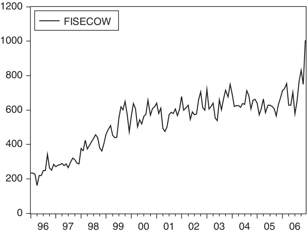
Figure 6.12 The monthly values of the fiscal labor costs in the company REX, in the years 1996–2006 (in PLN per one employee22).

Figure 6.13 The quarterly values of the company REX’s fiscal labor costs, in the years 1996–2006 (in PLN per one employee).

Figure 6.14 The annual fiscal labor costs in the company REX, in PLN per one employee.
Significant seasonal fluctuations of the tax burdens, resultant from the seasonality of the net sales income, are quite natural here. The demand’s specification occurring in the industry is the root cause of the seasonality of both, the fiscal charges to the labor costs per one employee as well as the burden of the VAT tax counted per one employee.
A study of the impact of the tax burdens on the changes of the company REX’s employment volume was conducted. The possibility of autoregressive dependencies of a trend occurrence and of seasonal fluctuations were also taken into consideration. An econometric linear model based on monthly data, covering 132 statistical observations from January 1996 to December 2006, was constructed. In the model the following variables occurred:
- EMPL – the average monthly number of employees,
- EMPL−1, …, EMPL−12 – the variable EMPL delayed adequately from 1 to 12 months,23
- AVAT, AVAT−1, …, AVAT−12 – the value of the VAT tax in PLN per one employee monthly in a current month and the delayed values adequately from 1 to 12 months,
- FISECOW, FISECOW−1, …, FISECOW−12 – the value of the fiscal labor costs in PLN counted per one employee monthly in a current year and the delayed value adequately from 1 to 12 months.24
The empirical model demonstrated in Table 6.3 was obtained as a result of numerical calculations.
Table 6.3 The empirical monthly econometric model describing the changes in the company REX’s employment dynamics, depending on the fiscal factors.
| Dependent variable: EMPL | ||||
| Method: least squares | ||||
| Date: 03/25/2014, time: 14:52 | ||||
| Sample(adjusted): 1996:12 2006:12 | ||||
| Included observations: 121 after adjusting endpoints | ||||
| Variable | Coefficient | Standard error | t-Statistic | Probability |
| C | 2.059000 | 1.028113 | 2.002698 | 0.0476 |
| EMPL(−1) | 0.940299 | 0.082076 | 11.45641 | 0.0000 |
| EMPL(−2) | −0.326948 | 0.108716 | −3.007367 | 0.0032 |
| EMPL(−3) | 0.331766 | 0.080076 | 4.143147 | 0.0001 |
| VATOW(−11) | 0.000680 | 0.000221 | 3.076332 | 0.0026 |
| FISECOW | −0.007940 | 0.001700 | −4.669978 | 0.0000 |
| FISECOW(−1) | 0.004921 | 0.001725 | 2.853569 | 0.0051 |
| R-squared | 0.895239 | Mean dependent var | 18.01653 | |
| Adjusted R-squared | 0.889725 | S.D. dependent var | 3.214507 | |
| S.E. of regression | 1.067462 | Akaike info criterion | 3.024556 | |
| Sum squared resid | 129.9002 | Schwarz criterion | 3.186296 | |
| Log likelihood | −175.9856 | F-statistic | 162.3651 | |
| Durbin–Watson stat | 1.933110 | Prob (F-statistic) | 0.000000 | |
The model is characterized by good stochastic qualities. The explanatory variables considered in the equation explain 89.5% of the total volatility of the single-base employment index. Empirical values of the employment index differ from their corresponding theoretical values, which were calculated on the basis of the equation from Table 6.3, by approximately one employee. The value of the Durbin–Watson statistic indicates that in the model, there is no autocorrelation of the random component (Figure 6.15).

Figure 6.15 The empirical and the theoretical (calculated on the basis of the model from Table 6.3) employment volumes (EMPL) as well as the residuals.
The biggest role in the formation of employment’s volatility in the enterprise plays autoregression, wherein autoregressive dependencies of the first, the second, and the third order have turned out to be statistically significant. This signifies employment inertia, wherein the impact of the employment level delayed by 2 months is characterized by a negative sign of the structural parameter’s assessment, which signifies commutativity of the fluctuations in a 2-month cycle. Autoregressive dependency of the first order is the strongest and it indicates that over 94% of the number of the employed in the previous month makes up current month’s employment.
The value of the tax on goods and services calculated per one employee delayed by 11 months positively influences the volume of employment. An increase in the burden of the VAT tax attributed to one employee entailed an employment increase after 11 months. The burdens of the fiscal costs of employment calculated per one employee negatively influence the current level of employment and positively influence it with a delay by 1 month. However, the sum of the parameter estimates along the variables FISECOW and FISECOW−1 is negative and equals to around −0.0012. This means that the overall relative growth of the burdens of the fiscal labor costs results in a decrease in employment volumes, in the considered here company REX.
In the above models, it has been shown that an excessive growth of the burdens of the fiscal costs to the wages in an enterprise produces consequences in the form of a decline in the demand for labor. Also, the excessive amounts of the tax on goods and services, in a small-sized enterprise, result in a decrease in the level of employment. An increase in the VAT rates causes a decrease in the demand, which results from risen prices of the commodity. Smaller production requires less employment, which ultimately was revealed by the above presented econometric models.
6.2 Econometric modeling of labor intensity of production
Labor-intensity of production as well as labor efficiency belong to a common family of economic categories; one is an inverse of the other.25 Each of those concepts is adequately relevant in an enterprise, providing it with information of a diverse, but a mutually complementary purpose. Ability to measure efficiency and labor intensity is a prerequisite for an accurate diagnosis of the situation and an appropriate support of the ownership decisions in a small company.
A known weakness of Polish small-sized enterprises is their informational negligence. The essence of this neglect lies in the lack of the time-series important for decision-making, which ought to be accumulated to improve decision-making processes. Even the mandatory information, including all the data related to statutory accounts, is not joined together into appropriate series of statistical data. All the more, we cannot speak about its appropriate processing, to prepare the foundations for at least rational decisions. Diagnosis of the situation as well as analysis and prediction of important changes in the enterprise is extremely difficult.
In this part of the book, the tendencies of the changes in the labor intensity of production in a small-sized enterprise will be presented. Depending on the manner of defining the numerator and the denominator of the labor-intensity formula (LC = L/P), various volumes of different economic sense can be obtained. Let us consider two concepts of the labor input (L) in a small company and four conceptual formulas of the production (P).
In Table 6.4 and Figure 6.16, the time series of labor intensity of production in a small-sized enterprise,26 expressed in monetary units, were demonstrated. Labor input, appearing in the numerator, represents the annual, quarterly, or monthly labor costs. The production volume, appearing in the denominator, stands for the net sales income, the cash inflows, the gross sales income, and the values of the finished ready-made production in the sales prices. As such, the numbers in Table 6.4 represent the annual labor costs (in PLN) attributed to one thousand of the production value in one of the meters listed here.
Table 6.4 The company REX’s labor intensity of production in monetary27 units (annually).
Source: The company’s documentation.
| Year | LABCN | LABCC | LABCB | LABCP |
| 1996 | 122.8571 | 102.2092 | 106.9026 | 114.8168 |
| 1997 | 169.5511 | 146.7834 | 147.2799 | 167.2178 |
| 1998 | 237.0013 | 228.9064 | 205.7237 | 225.8646 |
| 1999 | 211.2210 | 199.5265 | 183.7073 | 237.7567 |
| 2000 | 238.3379 | 207.7849 | 208.5811 | 234.7235 |
| 2001 | 254.1660 | 242.9409 | 222.8236 | 263.8387 |
| 2002 | 253.2822 | 226.4211 | 220.6642 | 250.9600 |
| 2003 | 267.2298 | 221.7364 | 233.6039 | 252.7890 |
| 2004 | 282.0118 | 219.2015 | 235.8800 | 249.8138 |
| 2005 | 298.8716 | 244.5517 | 245.1226 | 283.1824 |
| 2006 | 313.7652 | 243.3860 | 257.1385 | 315.9358 |

Figure 6.16 The company REX’s labor intensity of production in monetary units.
Source: Table 6.4.
Symbols in Table 6.4 are:
- LABCN – the cost of labor in PLN attributed to 1000 PLN of the company’s net sales income,
- LABCC – the cost of labor in PLN attributed to 1000 PLN of the cash inflows,
- LABCB – the cost of labor in PLN attributed to 1000 PLN of the gross sales income,
- LABCP – the cost of labor in PLN attributed to 1000 PLN of the finished ready-made production’s value.
In the years 1996–2006, a systematic increase in the labor costs attributed to 1000 PLN of the production value can be seen in each of the labor-intensity’s financial measures that were used. Especially in the 1990s, the labor intensities of a thousand of the production value, of the sales, and of the realization of the company’s28 receivables grew rapidly. Since 2000 the dynamics in each of the time-series considered here decreased significantly, approaching the saturation level. The best situation, from the perspective of the company’s interests, is observed in the labor intensity of the ready-made production, where after 2001 stabilization under this year’s level occurred.
Considering the financial measures of the labor involvement into manufacture and sale of a small-sized enterprise’s production, various upward tendencies of the above presented measures of the labor intensity can be noticed.
The labor intensity of production (of the manufacture and the sales), expressed in a natural measure of labor involvement, has been defined using four measures, which demonstrate the changes in the demand for labor, measured by the average annual number of job positions. These are as follows:
- LABCD – the average annual number of employees attributed to one manufacture of the ready-made production worth 1000,000 PLN,
- LABCB – the average annual number of employees attributed to 1000,000 PLN of the gross sales income,
- LABCN – the average annual number of employees attributed to 1000,000 PLN of the net sales income,
- LABCC – the average annual number of employees attributed to 1000,000 PLN of the cash inflows.
Statistical information about the labor intensity of production, based on the average annual employment, is presented in Table 6.5 and Figure 6.17. Since 1998, there is a marked drop in the demand for workers in the small enterprise. The emerged phenomenon of a decreasing demand for labor is a reaction to the effect of a dynamic increase in the labor cost during that period. Investments in the fixed assets of a substitution character, in terms of the labor factor, had the desired effect of reductions in the job positions needed in the company.
Table 6.5 The company’s labor intensity of production in natural units (annually).
Source: The company’s documentation.
| Year | LABCP | LABCB | LABCN | LABCC |
| 1996 | 15.79058 | 14.70215 | 16.89636 | 14.05667 |
| 1997 | 19.28739 | 16.98769 | 19.55652 | 16.93042 |
| 1998 | 18.81204 | 17.13452 | 19.73961 | 19.06539 |
| 1999 | 15.54954 | 12.01465 | 13.81407 | 13.04924 |
| 2000 | 13.75260 | 12.22090 | 13.96437 | 12.17426 |
| 2001 | 15.78865 | 13.33422 | 15.20982 | 14.53808 |
| 2002 | 13.84688 | 12.17529 | 13.97501 | 12.49293 |
| 2003 | 13.35549 | 12.34189 | 14.11843 | 11.71490 |
| 2004 | 13.44420 | 12.69432 | 15.17699 | 11.79673 |
| 2005 | 15.81584 | 13.69018 | 16.69208 | 13.65829 |
| 2006 | 15.28721 | 12.44219 | 15.18219 | 11.77674 |

Figure 6.17 The company REX’s labor intensity of production in natural measures.
Source: Table 6.5.
The econometric model of the labor intensity of production, based on the monthly data, describes the formation mechanism of the variable LABCD, which represents the value of the labor costs (in thousands PLN), attributed to 100,000 PLN of the ready-made production’s value (in the net sale prices) is presented in Table 6.6. The empirical econometric model, resultant from estimation of the parameters of the finished production workload model (LABCD, in monetary units), is presented in Table 6.6. In this model the following occur:
- LABCD(−11) – the monthly labor intensity of the ready-made production in monetary units delayed by 11 months;
- TAM(−5), TAM(−11) – the technical devices in machinery and equipment per one employee (in thousands PLN), delayed adequately by 5 and 11 months;
- MAR – the dummy variable taking the value of 1 in March of every year and the value of 0 in the remaining months;
- JUN – the dummy variable taking the value of 1 in June of every year and the value of 0 in the remaining months;
- AUG – the dummy variable taking the value of 1 in June of every year and the value of 0 in the remaining months;
- SEP – the dummy variable taking the value of 1 in June of every year and the value of 0 in the remaining months;
- OCT – the dummy variable taking the value of 1 in June of every year and the value of 0 in the remaining months.
Table 6.6 The parameter estimation results of the model for the labor intensity of the ready-made production, in monetary units (LABCD), based on monthly data.
| Dependent variable: LABCD | ||||
| Method: least squares | ||||
| Date: 03/25/2014, time: 15:49 | ||||
| Sample(adjusted): 1996:12 2006:12 | ||||
| Included observations: 121 after adjusting endpoints | ||||
| Variable | Coefficient | Standard error | t-Statistic | Probability |
| C | 110.8799 | 28.88057 | 3.839 256 | 0.0002 |
| LABCD(−11) | 0.362905 | 0.096687 | 3.753 395 | 0.0003 |
| TAM(−5) | 8.714928 | 2.741211 | 3.179 226 | 0.0019 |
| TAM(−11) | −5.194010 | 2.736619 | −1.897 966 | 0.0603 |
| MAR | 50.52375 | 25.28412 | 1.998 240 | 0.0481 |
| JUN | 89.00362 | 24.98374 | 3.562 461 | 0.0005 |
| AUG | 119.2980 | 27.58651 | 4.324 506 | 0.0000 |
| SEP | −75.15040 | 26.94066 | −2.789 479 | 0.0062 |
| OCT | −59.48777 | 25.76085 | −2.309 232 | 0.0228 |
| R-squared | 0.472216 | Mean dependent var | 292.3565 | |
| Adjusted R-squared | 0.434517 | S.D. dependent var | 96.92015 | |
| S.E. of regression | 72.88257 | Akaike info criterion | 11.48704 | |
| Sum squared resid. | 594929.3 | Schwarz criterion | 11.69500 | |
| Log likelihood | −685.9662 | F-statistic | 12.52602 | |
| Durbin–Watson stat | 2.054223 | Prob (F-statistic) | 0.000000 | |
In the model from Table 6.6, a positive autoregression of the 11th order occurs. Additionally, the technical devices in machinery and equipment delayed by 5 and 11 months (TAM)29 are the explanatory variables. Employment increased along with the growth of the variable TAM delayed by 5 months, and it decreased after 11 months from the increase in the technical devices in machinery and equipment. Based on that, a conclusion can be made that newer machinery and equipment encouraged a decrease in the company REX’s labor intensity after 11 months. The dummy variables also appeared, revealing periodic positive fluctuations: in March, in June, and in August as well as negative ones in September and in November. The positive periodic fluctuations result from the industry’s specificity, in which, especially from June till August, the demand for labor grows due to an increased demand for its products in autumn and winter time. It requires manufacture for store. Since September, the demand for work drops, as a result of storing the ready-made products manufactured in advance (Figure 6.18).

Figure 6.18 The actual and the theoretical monthly values of the company’s labor intensity of the ready-made production (in thousands PLN) as well as the residuals.
The fitting accuracy of the model can be considered as moderate.30 The coefficient of determination (R2 = 0.472) indicates that about 47.2% of the monthly volatility of the labor intensity of production is explained by the equation from Table 6.6. Also, the standard residual error (Su = 72.9) confirms that the random fluctuations of the labor intensity can be considered as moderate. The Durbin–Watson statistic (DW = 2.054) indicates that in the equation from Table 6.6, there is not any statistically important autocorrelation of the random component. These conclusions can be confirmed during analysis of Figure 6.19, which demonstrates the actual and the theoretical volumes of the ready-made production workload and the equation’s residuals.

Figure 6.19 The actual and the theoretical monthly values of the company’s labor intensity of the ready-made production (in persons/100 thousand PLN) as well as the residuals.
Table 6.7 The parameter estimation results of the model for the labor intensity of the ready-made production in natural units (LABCD), based on the monthly data.
| Dependent variable: LABCD | ||||
| Method: least squares | ||||
| Date: 03/25/2014, time: 16:08 | ||||
| Sample (adjusted): 1996:12 2006:12 | ||||
| Included observations: 121 after adjusting endpoints | ||||
| Variable | Coefficient | Standard error | t-Statistic | Probability |
| C | 7.722308 | 3.808304 | 2.027755 | 0.0449 |
| LABCD(−1) | 0.260855 | 0.075126 | 3.472237 | 0.0007 |
| LABCD(−11) | 0.390441 | 0.089307 | 4.371898 | 0.0000 |
| TAM(−5) | 0.581510 | 0.244232 | 2.380976 | 0.0189 |
| TAM(−10) | −0.670380 | 0.231987 | −2.889729 | 0.0046 |
| JUN | 6.772573 | 2.092653 | 3.236358 | 0.0016 |
| AUG | 6.680682 | 2.261812 | 2.953686 | 0.0038 |
| SEP | −6.278568 | 2.219735 | −2.828522 | 0.0055 |
| R-squared | 0.451951 | Mean dependent var | 20.88974 | |
| Adjusted R-squared | 0.418001 | S.D. dependent var | 8.029835 | |
| S.E. of regression | 6.125871 | Akaike info criterion | 6.526748 | |
| Sum squared resid. | 4240.472 | Schwarz criterion | 6.711593 | |
| Log likelihood | −386.8682 | F-statistic | 13.31225 | |
| Durbin–Watson stat | 1.906838 | Prob (F-statistic) | 0.000000 | |
Similarly to the above, we present an econometric model for the monthly labor intensity of production in natural units (the group of Figures 6.17). Downward trends of that labor intensity in natural units are noticed. In both groups of the monthly labor intensity measures some periodical fluctuations of large amplitude occur. The empirical econometric model of the monthly labor intensity of the ready-made productions in natural units is presented in Table 6.7.
In the equation from Table 6.7, the dependent variable (LABCD) was explained with a moderate accuracy by configuration of the considered explanatory variables. The coefficient R2 = 0.452 indicates that the set of explanatory variables of the considered equation explains 45.2% of the total volatility mass of the labor intensity. What is more, the actual values of the variable LABCD differ from its theoretical values that were calculated on the basis of this equation, on average, by slightly more than 6 persons per 100,000 PLN of the ready-made production’s value (Su = 6.1). The empirical Durbin–Watson statistic (DW = 1.907) indicates that in the considered equation, there is no autocorrelation of the random component. The description accuracy of the variable LABCD along with the sizes of the fluctuations (in the form of the residuals) is illustrated in Figure 6.19.
The model from Table 6.7 includes autocorrelation of the variable LABCD. The autoregressive dependencies of the 1st and the 11th order turned out to be statistically significant. Additionally, the technical devices in machinery and equipment with the delays of 5 and 10 months also played an important role in this equation. Both the character of the autoregression as well as the impact of the technical devices on the labor intensity are analogical to the results observed in the model presented previously in Table 6.6.
The monthly periodic fluctuations of the labor intensity of the ready-made production, expressed in a natural measure, are specific here. Labor-intensity’s positive deviations from the systematic component occurred in January and in August, while the negative ones in September. The positive as well as the negative deviations of the labor intensity were formed on the level slightly over six employees employed monthly per 100,000 PLN of the ready-made production.
The labor intensity of production in a small-sized enterprise has much significance. Its observation and analysis lead to various conclusions and decisions. The changes in the labor intensity are resultant from an impact of many factors, part of which is outside the enterprise and part within it.
Very strong impulses for the entrepreneur’s actions aimed at suppressing the growth of labor costs, attributed to one production unit; in Poland they appear through political decisions. They can include the changes in the Labor Code,31 regular minimum wage raises as well as increases in the social benefits, or an increase in the burden of the Social Security. Entrepreneurs react to those changes by initiating investment32 processes, which are aimed at substitution of the human labor with machinery and equipment. Thus, investments occur, which allow saving the human labor.
The result of the investments substituting human labor is a decline in the labor intensity of production, expressed in the number of employees attributed to a variously measured unit of production.33 Thus, by keeping the level of production, even by increasing it, the volume of employment in the enterprise can be limited. This process can be ascribed to the rapid growth of the unemployment rate in Poland, especially since the first half of the 1990s in the twentieth century.
6.3 Econometric model in selection of an efficient worker
Under the conditions of unemployment, attracting the right employee available on the labor market is not easy. Big corporations often engage specialized companies34 to search for suitable workers. Finding a candidate suitable for the job, even for a worker position, can pose difficulties. Choosing one from a group of many candidates requires experience, intuition, and having an adequate set of criteria necessary to make a rational decision.
Requirements for a candidate for a given job position can be defined in various ways. Some entrepreneurs rely on intuition, which is mostly based on his/her own experience. The below method of indicating the necessary qualities of a worker is based on statistical regularities observed in the activities of the entrepreneur himself/herself or in similar enterprises with the same type of job positions. Efficiency of the worker’s labor35 should be the criterion for assessing the worker’s suitability, measured by his/her individual labor efficiency. Having a homogenous data on individual labor efficiency of each employee and on their personal characteristics allows construction of an econometric model. Such model can serve as a good tool for selection of workers for a given type of job positions. An econometric model of individual labor efficiency can have the following from:
where
| yi | Individual labor efficiency of the ith employee (i = 1, …, n) |
| xi1, …, xij , …, xik | The explanatory variables representing personal characteristics of the ith employee |
| α0, α1, …, αj, …, αk | The model’s structural parameters |
| ηi | The random component |
| N | The number of employees, whose individual labor efficiency was measured |
Out of worker’s personal characteristics, the ones which differentiate him/her from other workers can be listed, for example:
- gender
- age
- profession
- education
- marital status
- family status
- place of residence
- owned assets.
Other personal characteristics can also be considered if there are indications pointing to the importance of those characteristics in crating the workers’ labor efficiency.
Measuring both the workers’ labor efficiency as well as their personal characteristics is essential for application of the decision-making tool indicated here. Measuring the individual labor efficiency can be troublesome, when some difficulties with establishment of a uniform and comparable efficiency measure of each employee36 occur as a result of work division. An experienced entrepreneur, however, can overcome this difficulty. Measuring employee’s personal characteristics is not easy though.
Quantification of measurable characteristics, using the numbers belonging to the relative scale, seems obvious. It is thus easy to measure the characteristics such as age, the number of the dependents, the number of children, the distance from the place of residence to the place of employment, the commute time, the number of years of education, seniority, and the value of his/her assets. However, using measurement in the relative scale is not always possible. Using a relative measurement is not always rational from the perspective of the study. In fact, measurement of the characteristics such as gender, marital status, profession, or education can be uncomplicated. Using the dummy variables makes it easy to measure each of the so-called qualitative characteristics.
Numerical expression of a personal quality, which is characterized by having only two variants, is least complicated. An example of such characteristic is the worker’s gender. Existence of two variants provides a possibility of using only one dummy variable, defined, for example, as follows:
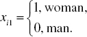
The parameter α1 then will provide information on by how much, on average, does labor efficiency of a woman differs compared to that of a man.37 A zero value of the parameter α1 indicates that labor efficiency of a woman does not differ – in the statistical sense – from that of a man.
Measuring the properties of the so-called immeasurable properties, when it is possible to distinguish many variants of a given characteristic, is much more difficult. A good example of that can be employee’s education. Various possibilities can be taken into account, such as, for example, elementary education, vocational education, medium school education, or higher degree education (bachelor and masters). In such case, there is no need of a simultaneous extraction of the dummy variables for each of the education variants specified, which can differentiate individual labor efficiency for a given job position. As such, we can define the following dummy variables representing a considered characteristic:


Defining many other dummy variables, representing employees’ education, is possible. Their application should arise from the needs of a particular study.
Let us suppose that the entrepreneur has in his disposition an empirical econometric model of individual labor efficiency, for the TXP in FP ALFA. This model has the following form38:
where39
ŷi – the amount of details XC, manufactured by the ith worker during a work shift,
xi1 – the dummy variable representing the worker’s age, defined as follows:

xi2 – the dummy variable describing gender:

xi3 – the variable characterizing the worker’s family situation, expressing the number of the dependents,
xi4 – the dummy variable indicating the worker’s marital status:

xi5 – the dummy variable representing education:

xi6 – the dummy variable describing vocational training, defines as follows:

xi7 – the dummy variable expressing the worker’s place of residence:

xi8 – the dummy variable, differentiating the workers’ financial status:

The empirical model 6.4 can be an effective tool for selecting workers for the TXP division in the company FP ALFA. It allows a preference of those people, among the many candidates for work, who possess personal characteristics fostering high individual labor efficiency. The model 6.4 suggests that among the candidates for work in the TXP division, those should be preferred who are characterized by the following personal characteristics:
- age up to 40 years;
- men;
- the candidates having a significant number of dependents;
- not having higher education;
- those who have completed a specialized vocational course;
- persons commuting to work from nearby cities/towns;
- who do not have any property.
The model 6.9 indicates that a worker with the abovementioned characteristics guarantees – in the statistical sense – the highest expected individual labor efficiency for the TXP division. However, some cases when the above diagnosis will not be fully accurate should be accounted for. At the same time, it is possible to define personal characteristics of a candidate for work, which are far less favorable for high labor efficiency.
Summing up, the empirical econometric model of individual labor efficiency for a given group of work positions can be an effective tool for selecting the candidates for employment in that place. By inserting the values of statistically significant personal characteristics of a candidate for work into the model, his/her potential individual labor efficiency (ŷip) can be obtained, similar to that obtained for the workers with comparable personal characteristics, employed in the same company in the past. Thus, it is possible to sort the candidates for the vacant job positions accordingly to their potential labor efficiency level. Ultimately, the one should be chosen whose potential efficiency is the highest, that is
where v is the number of the candidates, who applied for the job during recruitment, and ŷipw is the potential efficiency of the best candidate, with a given criterion of the choice.
A situation may arise when the employer establishes a minimal norm of potential labor efficiency (ŷpN). In such cases, only those candidatures will be considered who fulfill the condition ŷip ≥ ŷpN (i = 1, …, v). Then, it is possible that none of the candidates meets the employer’s requirement, that is, in all cases ŷip < ŷpN (i = 1, …, v). In such a state of things, none of the candidates will be employed, which results in repetition of the recruitment.
The structure of individual labor efficiency usually is characterized by a right-sided skewness. Therefore, approximately one-third of workers achieve the average arithmetic labor efficiency. At the same time, employment of a new worker with potential labor efficiency ![]() (where
(where ![]() represents the average arithmetic labor efficiency in the considered group of workers) will cause a decrease in its averaged value in the considered group of workers. In practice, however, it is difficult to find a person with labor efficiency
represents the average arithmetic labor efficiency in the considered group of workers) will cause a decrease in its averaged value in the considered group of workers. In practice, however, it is difficult to find a person with labor efficiency ![]() , who would guarantee maintenance or growth of the average team efficiency. Thus, it is worthwhile to make sure that the number ŷpN is at the level above the team efficiency’s median.
, who would guarantee maintenance or growth of the average team efficiency. Thus, it is worthwhile to make sure that the number ŷpN is at the level above the team efficiency’s median.
Selection of a candidate for a vacant job position can be done using a recursive model composed of two equations. The first equation will describe a formation mechanism of individual labor efficiency in a group of workers, according to their personal characteristics. The second equation will describe the principles of workmanship volatility of the products manufactured by this group of workers, according to their personal characteristics and their individual labor efficiency. A hypothesis can be posed that excessive emphasis on individual team-labor efficiency can result in a decrease in workmanship quality.
More precise information on the relations between labor efficiency and workmanship quality of the production manufactured by the workers and their personal characteristics is to be supplied by regression models. In our case, an econometric model composed of the following two equations will be considered:

where
| α1i, α2i | Structural parameters at the model’s predetermined variables (i = 0, 1, 2, 3, 4) |
| β12 | the structural parameter at the model’s interdependent variable |
| η1i, η2i | random components of the model’s equations |
Statistical data presented in Table 6.8 provides information about the quality of manufactured production (produced by each one of the 30 workers) during a given month (y1i), about individual labor efficiency (y2i) and about selected personal characteristics.40 The variable y1i (i = 1, …, 30) has characteristics of a dummy variable. It takes the value of 1 if the worker falls within the accepted standards of production shortages, and the value of 0 when the worker goes over the standard limit of the shortages predetermined for a given job position during a given time-period. Variable xi1 takes the value of 1 when the worker has vocational education and the value of 0 in the remaining cases. Variable xi2 represents gender; it takes the value of 1 for females and the value of 0 for males. Variable xi3 provides information about the workers’ age, expressed in the number of completed years of age. Variable xi4 provides information about work seniority, expressed in the number of full working years. The last variable xi5 provides information about the time of commuting to work from the place of residence, calculated in minutes.
Table 6.8 The worker’s efficiency and labor quality, as well as some of their personal characteristics.
Source: Contractual data corresponding with actual data.
| The worker’s id number (i) | Quality of manufactured production (y1i) | Labor-efficiency (in items) (y2i) | Education (xi1) | Gender (xi2) | Age (years) (xi3) | Seniority at work (xi4) | Commuting time (xi5) |
| (1) | (2) | (3) | (4) | (5) | (6) | (7) | (8) |
| 1 | 0 | 92 | 1 | 0 | 23 | 3 | 20 |
| 2 | 1 | 93 | 1 | 0 | 25 | 4 | 25 |
| 3 | 1 | 95 | 1 | 0 | 27 | 7 | 30 |
| 4 | 1 | 96 | 1 | 0 | 26 | 8 | 15 |
| 5 | 1 | 98 | 1 | 0 | 28 | 5 | 15 |
| 6 | 1 | 99 | 1 | 0 | 27 | 7 | 10 |
| 7 | 1 | 102 | 1 | 0 | 29 | 6 | 15 |
| 8 | 1 | 103 | 1 | 1 | 30 | 11 | 25 |
| 9 | 1 | 104 | 1 | 0 | 30 | 10 | 20 |
| 10 | 1 | 105 | 1 | 0 | 29 | 7 | 15 |
| 11 | 0 | 107 | 0 | 0 | 31 | 12 | 10 |
| 12 | 1 | 108 | 0 | 1 | 32 | 9 | 15 |
| 13 | 0 | 110 | 0 | 0 | 33 | 13 | 20 |
| 14 | 0 | 115 | 0 | 0 | 34 | 12 | 20 |
| 15 | 1 | 118 | 0 | 0 | 33 | 14 | 25 |
| 16 | 1 | 119 | 1 | 0 | 35 | 16 | 30 |
| 17 | 1 | 120 | 1 | 0 | 36 | 15 | 35 |
| 18 | 1 | 120 | 1 | 1 | 36 | 16 | 40 |
| 19 | 1 | 122 | 1 | 0 | 34 | 14 | 20 |
| 20 | 1 | 123 | 1 | 0 | 36 | 17 | 15 |
| 21 | 1 | 124 | 1 | 0 | 37 | 16 | 20 |
| 22 | 1 | 125 | 1 | 0 | 38 | 19 | 10 |
| 23 | 1 | 122 | 1 | 0 | 39 | 16 | 20 |
| 24 | 1 | 122 | 1 | 0 | 40 | 14 | 15 |
| 25 | 1 | 121 | 1 | 0 | 40 | 19 | 30 |
| 26 | 0 | 119 | 0 | 1 | 41 | 23 | 10 |
| 27 | 1 | 120 | 0 | 0 | 40 | 22 | 15 |
| 28 | 0 | 118 | 0 | 0 | 39 | 19 | 20 |
| 29 | 0 | 117 | 0 | 0 | 24 | 4 | 20 |
| 30 | 1 | 116 | 0 | 0 | 25 | 5 | 15 |
| ∑ | 23 | 3353 | 20 | 4 | 977 | 363 | 595 |
The first empirical equation describing the mechanism from the system of a 6.6-type, based on the statistical data from Table 6.8, has the following form:

Most of the explanatory variables from Equation 6.7 are characterized by statistical insignificance. After elimination of insignificant variables, we will get the following empirical equation describing volatility of workmanship quality in the considered group of workers41:

In Equation 6.8, the variable y2i is kept, although its significance can be considered at a mere significance level of γ = 0.28. However, variable y2i in Equation 6.8 provides important information, from the perspective of the company’s management. First of all, it does not confirm the hypothesis that an increase in labor efficiency decreases the products’ workmanship quality. On the contrary, an increase in labor efficiency improves the products’ workmanship quality, as a result of the workers’ increasing experience. Individual efficiency did not reach the critical level, beyond which labor quality deteriorates. What is more, Equation 6.8 also indicates that workers with vocational education produce better labor quality – compared to the workers with different education. Workers with vocational education realize defect-free production, on average by 58%, than the other education groups. This suggests that during selection of the worker for a vacant job position, those candidates should be preferred, who have vocational education, which will contribute to the quality of manufactured goods.
The random component of Equation 6.7 (and thus of Equation 6.8) is characterized by heteroscedasticity. Therefore, the Aitken’s estimator provided by Equation 1.55 will be more precise (effective) in this case. As such, it will be necessary to use the theoretical values of explanatory variable ŷ1i from Equation 6.7 to assign the weights wi calculated according to the formula 1.52. After estimating the parameters of the equation describing ŷ1i, using the Aitken’s estimator according to Equation 1.55, and with subsequent reduction in statistically insignificant variables, we get an empirical equation in the following form:

In the empirical equation 6.9, the value of the coefficient ![]() was higher in comparison with
was higher in comparison with ![]() . Moreover, empirical values of t-Student statistics at explanatory variables increased as well. Thus, variable y2i can be considered as statistically significant, with a risk of type I error that is slightly higher than before, that is, at the significance level of γ = 0.27. Decisional conclusions, resulting from Equation 6.9, are identical to those which emerged in reference to Equation 6.8.
. Moreover, empirical values of t-Student statistics at explanatory variables increased as well. Thus, variable y2i can be considered as statistically significant, with a risk of type I error that is slightly higher than before, that is, at the significance level of γ = 0.27. Decisional conclusions, resulting from Equation 6.9, are identical to those which emerged in reference to Equation 6.8.
An equation describing a volatility mechanism of individual labor efficiency affected by the considered personal characteristics has the following empirical form:

After elimination of the explanatory variables which are statistically insignificant, we get the following equation of individual labor efficiency:

It turns out that the worker’s age (xi3) is the only statistically significant variable impacting his/her individual labor efficiency. Over 63% of individual efficiency fluctuations result from variability of the workers’ age. Therefore, similarities between the distribution of individual labor efficiency and the structure of workers, in terms of their age, can be expected. Average labor efficiency at ![]() items is smaller than the medians of
items is smaller than the medians of ![]() items. This signifies left-sided skewness of labor efficiency’s distribution, which is confirmed by the coefficient of skewness equal to −0.548. Distribution of the workers according to their age is slightly left-skewed, since the average arithmetic age at
items. This signifies left-sided skewness of labor efficiency’s distribution, which is confirmed by the coefficient of skewness equal to −0.548. Distribution of the workers according to their age is slightly left-skewed, since the average arithmetic age at ![]() years is slightly smaller than the median, which is equal to
years is slightly smaller than the median, which is equal to ![]() . The skewness coefficient of the age structure is equal to −0.11. Staff is characterized by significant professional experience. The result of the workers’ age impacting their individual labor efficiency can be referred to the age range observed, that is, from 23 to 41 years of age. Thus, the group’s age range is 18 years. It is easy to calculate that the expected efficiency of a 23-year-old worker is
. The skewness coefficient of the age structure is equal to −0.11. Staff is characterized by significant professional experience. The result of the workers’ age impacting their individual labor efficiency can be referred to the age range observed, that is, from 23 to 41 years of age. Thus, the group’s age range is 18 years. It is easy to calculate that the expected efficiency of a 23-year-old worker is ![]() items monthly; while the expected labor efficiency of a 41-year-old worker will be about
items monthly; while the expected labor efficiency of a 41-year-old worker will be about ![]() items monthly.
items monthly.
In the case considered here, a vacant job position should be filled by a candidate in the age of 35–40 years, so he/she can achieve high labor efficiency. Moreover, it ought to be a candidate with vocational education, which increases the chance of better production quality.
It is worth keeping in mind that the result obtained in the above case is not universal. Comparable statistical information about labor efficiency and labor quality in given group of worker positions should be collected for every case. Knowledge of important personal characteristics which shape production quality and individual labor efficiency – for every case – allows reduction in the risk associated with erroneous employment decisions. The procedure offered here is meant to reduce the risk of faulty decisions. Each wrong personnel decision may result in additional costs for the company to incur. Other negative consequences, which companies want to avoid, may also emerge.
6.4 Econometric model in the selection of an efficient white-collar worker
The above proposed employee recruitment procedure can be used for every job position, for which the results of activity can be measured. In the enterprise, such position can be that of a salesman (sales person, sales representative, etc.), for whom the generated sales income will be the measure of his/her effectiveness. It is worthwhile to pay a bit of attention to the traders. A good trader activates the capital frozen in the merchandise. This provides an opportunity to recover the amounts engaged into production, thus increasing the capital by the values of income. An appropriately trained, efficient, and loyal sales representative can play a decisive role in the economic condition of the enterprise.
The entrepreneur should be aware of the role a trader plays in the company. Because of that, it is important to have the knowledge about the selection methods and the methods of assessing the salesperson’s work. The art of conversation combined with client psychology, negotiation techniques, the knowledge about trade agreements, are the principal issues, which the sales representative must be familiar with. Every salesperson should be skillful in those areas, regardless the sphere in which he/she sells the goods (services). A perfect knowledge of the subject for sale is also necessary.
Some personal characteristics foster salesperson’s work efficiency, others are obstacles in practicing this type of activity. An entrepreneur must be familiar with this dichotomy of traits. Knowledge of this can be acquired from an econometric model structured analogously to the model 6.4. The natural assessment measures of a salesperson’s labor efficiency can be the number of new clients acquired and the value of the sales or the profit earned by him/her from all transactions in a given period. Those measures can be used separately or jointly. In the econometric model, they will function as the dependable variable (y1i, y2i, or y3i), forming the criterion for assessment and for the choice of the trader.
The effects of a salesperson’s work must be associated with his/her personal characteristics. The characteristics indicated in Section 6.3 and those analyzed during the assessment of a worker’s job performance as well as other characteristics, which can affect the salesperson’s labor efficiency, should be considered. These will include both, objectively defined characteristics as well as subjective ones. Among the subjective ones, the following assessment types can be distinguished: a “handsome” salesman, a “good looking” sales woman, a representative “having good taste,” an “inventive” salesperson. The use of subjective characteristics, however, requires having a relatively objective system of testing those types of characteristics.
The objective characteristics of a salesperson, different from the ones previously considered in the models 6.3 and 6.4, can be as follows:
- possession of a driver’s license
- possession of a car
- possession of a phone
- Internet access and so on.
The entrepreneur must be able to identify the characteristics favoring or hindering the salesperson’s work efficiency. Some of those characteristics, which are considered to be important, in practice can turn out to be statistically insignificant. Information about this can be obtained from the empirical econometric model, which should be an incentive for its use.
Having an empirical econometric model of the economic work efficiency of a salesperson, describing the variable ypi(p = 1, …, P; i = 1, …, n), allows the use of a selection procedure for a given job position. An approach similar to the one described in Section 6.3 can be effective during a selection using the formula 6.5.
Labor-efficiency assessment in an office is one of those difficult issues, which always arouse all sorts of controversy. A good functioning of an enterprise, however, relies heavily on the efficiency of its office work. Therefore, selection of workers, who guarantees maximum work effectiveness on the job positions connected with the company’s organization and management, keeping the financial-accounting and technical documentation, supply, and so on, is of high priority.
Evaluation of intellectual work can be done intuitively. It is a most commonly used method. Often, however, this method is largely unreliable. Therefore, it is worth to use a score method, in which an adequate number of points for particular effects of the worker’s actions are determined. Using the score method for office work allows a discourse about the office worker’s efficiency. The number of the points scored (yib) is the measure of the office worker’s assessment; thus it can be the dependable variable in an econometric model of the worker’s effectiveness in this group. The set of dependable variables of such a model ought to be complementarily specified. These variables will represent the worker’s personal characteristics. Having an empirical econometric model of the office worker’s efficiency facilitates making right decisions regarding employing new people to replace the ones leaving or employing workers for newly opened job positions in a given group. The procedure of econometric modeling is then analogous to the proceedings relating to the model 6.4 and to a decision-making according to the formula 6.5.
In some cases, it is possible to apply worker’s assessment using the “beam” criteria. It is expected that the worker ought to be creative, be a good manager, be fair in evaluating subordinates, have good contacts with his/her coworkers, and so on. Each of these assessment components can be verbally defined so that the description is precise. The dummy variable (yiz) can then be the measure of such worker’s assessment, having the value of 1, when he/she fulfills all the requirements for each assessment criterion, and the value of 0, when he/she does not meet any of the conditions. The tool of choice may then be an econometric model with a dummy dependable variable, which allows estimation of the probability of meeting all the criteria of a worker’s assessment. Having such empirical model allows making a rational choice out of the candidates for the job, according to the formula 6.5. The selection, in this situation, is made according to the principle of the highest respect of the expected probability of meeting the criteria verbally defined.
Let us consider an example of using an econometric model for selecting a good candidate for the position of a trader in the enterprise. Table 6.9 contains statistical information about effectiveness of the traders’ work in the company MAX and information about some of evaluations of their personal characteristics. Work effectiveness of this group of workers, on one side, is measured by the value of the sales income obtained by issuing appropriate invoices in a given period and by timely payments for the sales resultant from those invoices, which makes up the company’s receivables. The measurement of the claims recovery was done using the dummy variables, defined as follows43:
- y1i – the dummy variable taking the value of 1 when in the sales network of the ith sales representative overdue44 receivables had emerged and the value of 0 in the opposite case.
Table 6.9 The effectiveness of claim recovery, the net sales income as well as the selected personal characteristics of the traders in the company MAX, annually for the years 2010–2013 (in thousands PLN annually)42.
Source: The company MAX’s data analogous to the actual data.
| Trader’s # (i) | y1i | y2i | xi1 | xi2 | xi3 | xi4 | xi5 | xi6 | xi7 |
| 1 | 0 | 872 | 1 | 0 | 3 | 0 | 0 | 24 | 0 |
| 2 | 0 | 880 | 0 | 0 | 3 | 0 | 0 | 25 | 0 |
| 3 | 0 | 900 | 0 | 0 | 2 | 0 | 0 | 23 | 0 |
| 4 | 0 | 910 | 0 | 0 | 4 | 0 | 2 | 25 | 0 |
| 5 | 0 | 912 | 0 | 0 | 3 | 0 | 1 | 27 | 1 |
| 6 | 0 | 930 | 1 | 1 | 5 | 0 | 1 | 26 | 1 |
| 7 | 1 | 933 | 0 | 0 | 5 | 0 | 1 | 28 | 1 |
| 8 | 0 | 940 | 0 | 0 | 5 | 1 | 3 | 27 | 0 |
| 9 | 0 | 945 | 1 | 1 | 3 | 0 | 0 | 29 | 0 |
| 10 | 0 | 950 | 1 | 0 | 4 | 0 | 0 | 30 | 0 |
| 11 | 0 | 952 | 1 | 0 | 7 | 0 | 1 | 30 | 0 |
| 12 | 0 | 955 | 0 | 0 | 6 | 0 | 1 | 29 | 0 |
| 13 | 0 | 960 | 0 | 1 | 5 | 0 | 1 | 31 | 1 |
| 14 | 0 | 966 | 0 | 0 | 8 | 0 | 1 | 32 | 0 |
| 15 | 0 | 967 | 0 | 0 | 6 | 0 | 2 | 33 | 0 |
| 16 | 0 | 968 | 1 | 0 | 8 | 1 | 1 | 34 | 0 |
| 17 | 0 | 970 | 0 | 0 | 8 | 1 | 2 | 33 | 0 |
| 18 | 1 | 985 | 0 | 1 | 7 | 0 | 1 | 35 | 1 |
| 19 | 0 | 990 | 0 | 0 | 9 | 0 | 1 | 36 | 1 |
| 20 | 0 | 992 | 1 | 0 | 8 | 0 | 2 | 36 | 0 |
| 21 | 0 | 998 | 1 | 0 | 9 | 0 | 2 | 34 | 1 |
| 22 | 0 | 1000 | 0 | 0 | 9 | 0 | 3 | 36 | 1 |
| 23 | 1 | 1020 | 0 | 1 | 7 | 0 | 1 | 37 | 1 |
| 24 | 0 | 1025 | 0 | 0 | 8 | 1 | 2 | 38 | 0 |
| 25 | 0 | 1030 | 0 | 0 | 9 | 1 | 2 | 39 | 1 |
| 26 | 0 | 1060 | 1 | 0 | 10 | 0 | 3 | 40 | 1 |
| 27 | 0 | 1100 | 1 | 1 | 10 | 1 | 3 | 40 | 0 |
| 28 | 0 | 1160 | 0 | 1 | 11 | 1 | 4 | 41 | 0 |
| 29 | 1 | 1204 | 0 | 0 | 12 | 0 | 4 | 40 | 0 |
| 30 | 0 | 1260 | 0 | 1 | 11 | 1 | 2 | 39 | 1 |
The remaining symbols representing the variables listed in Table 6.9 are as follows:
- y2i – the annual net sales income obtained by this ith trader (in thousands PLN),
- xi1 – the dummy variable, representing the trader’s gender, taking the value of 1 for women and of 0 for men,
- xi2 – the dummy variable, providing information on competitive sports practiced by the trader, taking the value of 1, when he/she had practiced sports professionally and the value of 0, in the opposite case,
- xi3 – seniority in the trader position, expressed by the number of working years,
- xi4 – the dummy variable, informing about the trader’s economic education, taking the value of 1, when the trader has economic education and the value of 0, when he/she does not have such education,
- xi5 – the number of the trader’s dependents,
- xi6 – the trader’s age, expressed by the number of completed years of life,
- xi7 – the dummy variable, providing information about an educational status, taking the value of 1, when the trader has higher education and the value of 0, when he/she does not have such education.
More precise information about labor-efficiency relations and about the quality of production done by the workers along with their personal characteristics are provided by the regression models. In our case, a recursive econometric model composed of two equations is the subject of discussion:
where
| α1i, α2i | The structural parameters along the model’s predetermined variables (i = 0, 1, …, 7) |
| β12 | The structural parameter along the model’s total interdependent variable |
| η1i, η2i | The model’s random components |
Recursiveness of the hypothetical econometric model results from the assumption that targeting high amounts of the sales income obtained by the trader lowers his/her attention to the timeliness of settling by the clients their liabilities. In commercial practice, it happens that over-intensification of the sales causes delays in settling the payments for the invoiced goods and services.
Using the data presented in Table 6.9, an empirical probability function was obtained, which describes the mechanism of an occurrence frequency of the trader’s abnormal overdue claims, depending on his/her personal characteristics and the obtained sales income. It has the following form45:

Most of the dependable variables of Equation 6.14 are the variables statistically insignificant. Therefore, in the following estimations, reduction was performed. As a result, an empirical model with acceptable decision-making qualities has emerged:

The empirical Goldberger’s equation explains only 23% of the volatility of the dependable variable characterizing the formation of the overdue46 claims. Three (out of eight) explanatory variables differentiate the frequency of formation of the overdue claims in the traders’ activity. The results obtained can serve in the decision-making process during recruitment for a vacant job position in the sales department as well as in implementation of staff training. This means that effectiveness of the trader’s claim recovery does not depend on the amount of the sales income generated by him/her.
Similarly to the case of Equations 6.7 and 6.8, heteroscedasticity of the random components also occurs in Equations 6.14 and 6.15. This signifies a possibility of improving the estimative precision through application of the Aitken’s method for assessment of the parameters in Equation 6.12. As in the previous case, the weights wi were assigned on the basis of the theoretical values of ŷ1i, determined from Equation 6.14, using the formula 1.52. As a result of the calculations estimating the parameters in Equation 6.14 and of elimination of statistically insignificant variables, the following empirical equation was obtained:

The results obtained are more accurate, compared to Equation 6.15, as evidenced by empirical values of t-Student statistics and by a better value of ![]() . The conclusions emerging from the empirical equation 6.16 are the same as those emerging from Equation 6.15.
. The conclusions emerging from the empirical equation 6.16 are the same as those emerging from Equation 6.15.
An equation describing the impact of the traders’ personal characteristics on the generated sales income by them is as follows47:
Su = 88.88tys.zł, V = 8.49%, R2 = 0.778
Equation 6.10 shows that the sales income generated by a trader depends on xi2 (the dummy variable providing information about the fact of practicing competitive sports by a trader), on xi3 (the seniority in the trader’s profession expressed by the number of working years), as well as on xi6 (the trader’s age).
The system of Equations 6.12 and 6.13 can be used in employment decision-making, in case of a vacant trader job position in the enterprise. Having information about the candidates, it should be noticed that the most important trader characteristics influencing the sales income generated by a given trader are as follows: the fact of practicing competitive sports, seniority in trading, and the age. This allows using Equation 6.17, assessment of potential efficiency for each of the candidates for the job. Employment decision can be then made accordingly with the formula 6.5. In case of similar values48 of ŷ2ipw for two or more candidates, Equation 6.16 should be additionally used, which will indicate a candidate of a smaller risk of creating overdue claims, that is, of the smallest forecast value of the frequency of exceeding the allowed payment due dates ŷ1ipw. A candidate selected in this way is laden with the smallest risk of a faulty decision about the staff. There is no guarantee that ultimately, the candidate will satisfy the expectations during the tasks entrusted to him/her. Selection of each of the remaining candidates will be even more risky, compared to the case indicated using the empirical set of equations.