
5
Econometric modeling in management of small-sized enterprise
5.1 The concept of financial liquidity and its measurement in a small-sized enterprise
Financial liquidity of an enterprise is fundamental for its viability and development.1 Liquidity plays a particular role in a small-sized enterprise, which during the time of transformation in Poland faced the banks and their reluctance to grant credit, which is a liquidity buffering tool. As such, financial liquidity of a small-sized enterprise depends on the company’s ability to sell its products and to execute liabilities for the goods and services sold. Possible cash shortages are rarely complimented by bank loans. Typically, such supplementation comes from own funds of the company’s owner and of his family, including the amounts accumulated earlier on as a result of having the so-called periodical excess financial liquidity.
Manufacture of the goods for sale requires possession of necessary cash funds,2 which in turn come from the sale of the goods for which payment has been made, at the same time closing the circular cycle of capital.4 Production of the goods allows their delivery to the customers, which results in issuance of adequate invoices creating the receivables. After the time specified in an agreement, payment for the goods sold follows. This enables initiation of the next production cycle. The mechanism described here is presented in Figure 5.1.

Figure 5.1 The links between cash inflows, gross sales income, and ready-made production in a small-sized enterprise.3
Source: Own studies.
Completion of production allows a possibility of generating the sales income, which results in adequate cash inflows. Between:
- the ready-made production and the sales income,
- the sales income and the cash inflows, and
- the cash inflows and completion of ready-made production.
various time intervals occur.
In a small-sized enterprise, monthly and quarterly data are the most important time series related to cash settlements. These intervals are most crucial due to the frequency of implementing the company’s various commitments (from a time interval of one month to around three months).
Study of an enterprise’s financial liquidity uses a variety of tools of an indicating character. Typically, measurement is done during a predetermined time-period or – for comparison – over two time-periods. Information that is obtained essentially is statistical in character, as a result of which it is very poor and of a little use in financial management.
In a small-sized enterprise, access to information is much more difficult. Owners of this type of companies do consider the data from the past as important. They only collect information which they are obliged by law to keep on their records. Meanwhile, possession of some information from the past, in the form of sufficiently long time series, especially monthly ones, can simplify management of the company in various areas. Past financial characteristics as well as those reflecting intensity of the sales and of the manufacturing process are particularly important.
One of the most significant problems of a small-sized enterprise is having the cash necessary for timely payments of liabilities. In a small-sized company, scarcity of statistical data causes liquidity to play a particular role. Financing business activity in a small business entity, usually, is done by own funds. Very rarely such company uses a bank loan. During the entire time after 1990, the company encountered reluctance of Polish banks to grant credit loans constituting buffering tools for companies’ liquidity.
Multitude of the measures of financial liquidity5 does not mean it is always possible to use them, especially in a microenterprise. Lack of adequate statistical information is the main difficulty. Keeping simplified accounting in a small-sized enterprise is uncomplicated. The price behind this simplicity is unavailability of important information that would enable a precise diagnosis of the situation and evaluation of the past and the future.
Information collected about the company’s cash inflows and the value of the finished ready-made production6 is beneficial to its owners. It allows, inter alia, an approximate account of the company’s financial liquidity. Comparison of the cash amounts resultant from realization of receivables with the value of ready-made production7 provides a relatively precise picture of the company’s liquidity. The symbol casht denotes the value of cash inflows, while prodt denotes the value of finished production (in net sales prices). Comparison of those variables’ amounts in a given period, allows assessment of the company’s current financial liquidity. Only the manner of those variables’ comparison (the variable casht with the variable prodt) requires consideration. The first option entails comparison of the values of simultaneous cash inflows with the value of finished ready-made production.8 If there is inequality: casht ≥ prodt (t = 1, …, n), then the enterprise has the cash funds necessary to cover the liabilities during a t period. When cash < prodt it can signify deficiency of cash funds. It is worth noting though, that an entrepreneur, who must rely primarily on his/her own foresight, can accumulate cash funds during the periods of its surplus over liabilities, and can use it during a current shortage. As such, a better analytical solution involves examining the cumulated value of the cash funds in subsequent periods of a given year and its comparison with the cumulated value of ready-made production.
As a result, we are going to use three measures of a small-sized company’s liquidity in this work. The first of these measures will be the difference between the cumulated monthly cash inflows and the cumulate of the finished ready-made production,9 that is:
where:
An alternative measure of the cumulated monthly financial liquidity is going to be the relative measure of this liquidity for the current production. It is calculated using the following formula:
Variable liqproct is expressed in percentage points. It provides information on what percentage of the finished production’s value in a t month constitutes the value of the enterprise’s cumulated monthly financial liquidity.
Next measure of a small-sized company’s financial liquidity can be the ratio of cumulated cash inflows and cumulated finished production’s value, that is, an indicator of relative liquidity for the cumulated production:

Measure 5.3 contains information similar to that in measure 5.2. It is also expressed in percentage. It provides information on whether in a given month cumulated cash inflows were higher than cumulated finished production’s value and if so, by what percentage. Positive value of an observation on liqrelt indicates by what percentage the cumulated cash inflows were higher than the cumulated finished production’s value, in a given month. Negative value of liqrelt informs about the risk of a lack of liquidity, although not always.10
5.2 econometric modeling of monthly financial liquidity
A study of a small-sized manufacturing enterprise’s monthly financial liquidity was done from January 1996 to December 2006. Time series of the variables liq and liqproc are presented, respectively, in Figures 5.2 and 5.3. Significant seasonal fluctuations of cumulated liquidity expressed in monetary units as well as fluctuations of relative liquidity expressed in percentage were noticed. However, downward amplitude of seasonal fluctuations, indicating progressive stabilization of liquidity understood as such, can be seen. What is more, both liquidity measures are positive during most periods, while during many periods they are higher than zero. This signifies a generally good or a very good financial condition in the company.

Figure 5.2 Monthly financial liquidity of the company REX during the years 1996–2006 (in thousands PLN).

Figure 5.3 The structure of monthly cumulated financial liquidity of the company REX during the years 1996–2006 (in thousands PLN).
Figures 5.3 and 5.4 show the structure of the enterprise’s valuable financial liquidity and its relative financial liquidity during the years 1996–2006. While distribution of liquidity, expressed in its value, can be visually evaluated as close to normal, distribution of relative liquidity is visibly right-skewed. The average size of liquidity expressed in value was close to 106 thousands PLN, while the volume of relative liquidity – over 31%. Still, the company’s averagely very good financial condition cannot lead to the owners’ self-reassurance that everything is under control. All it takes is lack of financial liquidity (negative values) during few subsequent periods in order to cause significant difficulties in running the company. When the values are less than zero, the company faces the risk of bankruptcy.

Figure 5.4 Cumulated monthly financial liquidity of the company REX during the years 1996–2006 (in% %).
A detailed analysis of liquidity time series allows inference, that during 7 out of the 132 months liquidity measures were negative. The worst situation occurred during the period from September to December 1998, since financial liquidity measures were negative during four subsequent months. However, these values were below zero, which did not pose any threat for the company’s viability. During the worst financial month, the cumulated value of cash inflows was lower than the value of the finished ready-made production,11 by a mere 6.37%. In turn, during a subperiod between the years 1999–2006, the company’s financial liquidity measure was negative only during 1 month (January 2004).
At the same time, during many periods the company was characterized by an excess financial liquidity. During 29 out of the 132 months the company had an excess of cumulated cash inflows over the cumulated value of the finished ready-made production by 210%. Therefore, during the months of significant excess liquidity it was possible to accumulate cash funds. It is quite interesting, that excess liquidity usually occurred in the first three to five months of calendar year. As an exception, in 2003 and 2004, liquidity during the first months was grossly higher compared to the months of the second half-year.
Finally, large dispersion of the financial liquidity’s measures is noteworthy. Standard deviations of both variables reached relatively high values. However, it was mainly a differentiation between normal liquidity and excess financial liquidity (Figure 5.5).

Figure 5.5 The structure of cumulated relative monthly financial liquidity in the company REX during the years 1996–2006 (in%%).
The mechanism of the company’s monthly financial liquidity expressed by the variable liq is described by the empirical dynamic econometric model, written in Table 5.1.
Table 5.1 An empirical dynamic econometric model of the company’s financial liquidity liq, based on the monthly data for the years 1996–2006.
| Dependent variable: liq | ||||
| Method: least squares | ||||
| Date: 10/31/2008; time: 19:17 | ||||
| Sample(adjusted): 1997:01 2006:12 | ||||
| Included observations: 120 after adjusting endpoints | ||||
| Variable | Coefficient | Standard error | t-Statistic | Probability |
| C | 48.21616 | 14.12626 | 3.413230 | 0.0009 |
| liq(−1) | 0.797203 | 0.047525 | 16.77429 | 0.0000 |
| liq(−5) | −0.161817 | 0.047803 | −3.385088 | 0.0010 |
| liq(−12) | −0.146115 | 0.052655 | −2.774944 | 0.0066 |
| sbrut(−2) | 0.209423 | 0.073306 | 2.856831 | 0.0052 |
| sbrut(−10) | −0.211553 | 0.073948 | −2.860841 | 0.0051 |
| sbrut(−12) | 0.322061 | 0.082158 | 3.920044 | 0.0002 |
| jan | −54.74449 | 19.66362 | −2.784050 | 0.0064 |
| sep | −110.3969 | 24.51906 | −4.502495 | 0.0000 |
| oct | −150.1994 | 24.64126 | −6.095444 | 0.0000 |
| nov | −98.59027 | 26.32944 | −3.744488 | 0.0003 |
| t*jan | −1.211317 | 0.262139 | −4.620888 | 0.0000 |
| t*feb | −0.344235 | 0.134695 | −2.555660 | 0.0121 |
| t*jul | −0.349798 | 0.135516 | −2.581222 | 0.0113 |
| t*sep | 0.565260 | 0.260045 | 2.173703 | 0.0320 |
| t*oct | 1.117471 | 0.266116 | 4.199190 | 0.0001 |
| t*nov | 0.776393 | 0.273300 | 2.840812 | 0.0054 |
| R-squared | 0.828659 | Mean dependent var | 108.3792 | |
| Adjusted R-squared | 0.802043 | S.D. dependent var | 61.30909 | |
| S.E. of regression | 27.27783 | Akaike info criterion | 9.580596 | |
| Sum squared resid | 76640.24 | Schwarz criterion | 9.975491 | |
| Log likelihood | −557.8358 | F-statistic | 31.13388 | |
| Durbin–Watson statistic | 2.079405 | Prob (F-statistic) | 0.000000 | |
In the model presented in Table 5.1, autoregressive dependencies as well as the following variables occur: t* – the time variable representing the number of the month (t* = 1, …, 132); sbrut−2, sbrut−10 i sbrut−12 – the value of the gross sales income, appropriately delayed by 2 months and by 10 and 12 months. A separate group of exogenous variables consists of the dummy variables, taking the value 1 during the indicated month and the value of 0 during the remaining periods. The following symbols represent the dummy variables, distinguishing by number 1: jan – January, feb – February, mar – March, apr – April, may – May, jun – June, jul – July, aug – August, sep – September, oct – October, nov – November.12
The empirical equation demonstrated in Table 5.1 indicates that first-order autoregression forming the current sequential liquidity is crucial in the formation of the variable liqt. Commutativity of this variable’s volatility is formed by autoregressive dependencies of the 5th and 12th order. Gross sales income constituting a gross sum of the invoices issued during a given month, converted into the cash inflows, play a significant role in formation of the company’s financial liquidity. Time-constant seasonal fluctuations are adjusted by adequately variable seasonality, which ultimately results in a decrease of the amplitude of seasonal fluctuations during the following years. The actual and the theoretical values of monthly financial liquidity in the company REX as well as the residuals, calculated on the basis of the equation considered here, are presented in Figure 5.6.

Figure 5.6 Empirical and theoretical values of monthly financial liquidity liq in the company REX13 as well as the residuals during the years 1996–2006 (in thousands PLN), calculated on the basis of the equation given in Table 5.1.
An alternative dynamic empirical model describes the variable liqproc. It has the empirical form14 shown in Table 5.2. This model describes a volatility mechanism of the company’s relative financial liquidity in a very simplified way. There is a variable describing only the first-order autoregression, which indicates sequencing in the variable liqproc’s formation. What is more, very large positive constant seasonality in January as well as a significant positive seasonality in March appears. January’s constant seasonality is systematically decreased by a time variable correcting its seasonality. The actual and the theoretical values of cumulated relative monthly financial liquidity in the company REX as well as the residuals, calculated on the basis of the equation from Table 5.2, are shown in Figure 5.7.
Table 5.2 An empirical dynamic econometric model of the company’s financial liquidity, based on monthly data from the years 1996–2006.
| Dependent variable: liqproc | ||||
| Method: least squares | ||||
| Date: 12/17/2007; time: 10:48 | ||||
| Sample (adjusted): 1996:02 2006:12 | ||||
| Included observations: 131 after adjusting endpoints | ||||
| Variable | Coefficient | Standard error | t-Statistic | Probability |
| C | 3.748842 | 1.906265 | 1.966591 | 0.0514 |
| liqproc(−1) | 0.661443 | 0.041386 | 15.98223 | 0.0000 |
| jan | 120.0150 | 10.48327 | 11.44824 | 0.0000 |
| MAR | 13.71131 | 4.863916 | 2.818987 | 0.0056 |
| t*jan | −0.881299 | 0.137312 | −6.418243 | 0.0000 |
| R-squared | 0.770874 | Mean dependent var | 30.30581 | |
| Adjusted R-squared | 0.763600 | S.D. dependent var | 30.77835 | |
| S.E. of regression | 14.96474 | Akaike info criterion | 8.286691 | |
| Sum squared residual | 28216.86 | Schwarz criterion | 8.396431 | |
| Log likelihood | −537.7782 | F-statistic | 105.9789 | |
| Durbin–Watson statistic | 2.307237 | Prob (F-statistic) | 0.000000 | |
Figure 5.7 Empirical and theoretical values of monthly financial liquidity in the company REX (calculated on the basis of the equation from Table 5.2) as well as the residuals, during the years 1996–2006 (in%%).
The presented here simplified method of calculating and modeling a small-sized enterprise’s financial liquidity is characterized by accuracy sufficient for the company’s current management purposes. Using only adequately prepared graphs allows visual evaluation of the liquidity measures applied and of the scales of seasonal fluctuations. Using adequate and not very complicated econometric models will allow the owner to predict the scale of future financial liquidity. At the same time, it will be possible to adequately prepare for the expected liquidity levels, which may require appropriate accumulation of cash funds, in order to preserve security of the production process. It also becomes possible to indicate the periods, in which it will be relatively easy to finance investment purchases from the owner’s own funds.
5.3 econometric modeling of quarterly financial liquidity
The quarterly financial liquidity accounting is connected to the payment due dates (almost three-months-long) specified in the settlements for the suppliers of basic raw materials needed for production. Liabilities to the supplier of electricity are settled every two months. Sufficiently precise information about quarterly liquidity can refer to statutory liabilities15 such as: income tax, the tax on goods and services, and property tax. Analysis of liquidity during period of three months seems to be appropriately accurate and significant for most payments arising in connection with small-sized enterprise’s business activity.
The mechanism of quarterly financial liquidity in the company REX was described using two stochastic equations. The first empirical equation is specified in Table 5.3. In the equation from Table 5.3, the symbols: sbrut(−1) represent gross sales income delayed by 1 quarterly, snet and snet(−3) – current and delayed by 3 quarters net sales income, prod, prod(−1) – current and delayed by 1 quarter volumes of the company’s financial liquidity (Figure 5.8).
Table 5.3 An empirical dynamic econometric model of the company’s financial liquidity (liq), based on quarterly data from the years 1996–2006.
| Dependent variable: liq | ||||
| Method: least squares | ||||
| Date: 01/19/2008; time: 10:31 | ||||
| Sample(adjusted): 1996:4 2006:4 | ||||
| Included observations: 41 after adjusting endpoints | ||||
| Variable | Coefficient | Standard error | t-Statistic | Probability |
| C | 111.3354 | 36.81731 | 3.023995 | 0.0047 |
| sbrut(−1) | 0.637303 | 0.093277 | 6.832402 | 0.0000 |
| liq(−1) | 0.207248 | 0.102916 | 2.013761 | 0.0520 |
| snet | 0.674523 | 0.113202 | 5.958589 | 0.0000 |
| snet(−3) | 0.151101 | 0.065464 | 2.308146 | 0.0272 |
| prod | −0.924006 | 0.164212 | −5.626896 | 0.0000 |
| prod(−1) | −0.653855 | 0.160410 | −4.076157 | 0.0003 |
| R-squared | 0.708044 | Mean dependent var | 124.9390 | |
| Adjusted R-squared | 0.656522 | S.D. dependent var | 61.49152 | |
| S.E. of regression | 36.03833 | Akaike info criterion | 10.16130 | |
| Sum squared residual | 44157.89 | Schwarz criterion | 10.45386 | |
| Log likelihood | −201.3066 | F-statistic | 13.74263 | |
| Durbin–Watson statistic | 2.009039 | Prob (F-statistic) | 0.000000 | |

Figure 5.8 The structure of quarterly financial liquidity in the company REX during the years 1996–2006 (in%%).
The equation demonstrated in Table 5.3 explains 70.8% of the volatility of quarterly financial liquidity in the company REX. Liquidity measured in such way is characterized by an autoregression of the first order. There is a positive impact of the simultaneous net sales income and of the gross sales income delayed by 1 quarter. This means, that higher frequency of visiting the customers fosters improvement of the company’s financial liquidity. There is also a slight positive impact on improvement liquidity of the net sales income16 delayed by three quarters. Moreover, there is a negative impact on liquidity of the current and the delayed by 1 quarter value of the finished ready-made production. Manufacturing of ready-made production requires having the cash funds for its financing. Therefore, an increase of ready-made production’s value results in a decrease of quarterly liquidity. Figure 5.9 illustrates the actual and the theoretical quarterly values of the variable liq in company REX as well as the equation’s residuals.

Figure 5.9 Empirical and theoretical values of relative monthly financial liquidity in the company REX as well as the residuals (calculated on the basis of the equation from Table 5.3), during the years 1996–2006 (in%%).
An empirical equation describing a quarterly volatility mechanism of financial liquidity (liqrelt) has the form presented in Table 5.4. In the equation from Table 5.4, the symbols S1, S2, and S3 represent the dummy seasonal variables, taking the values of 1, respectively, in the following quarters: the first, the second, and the third as well as the values of zero in the remaining quarters.
Table 5.4 An empirical dynamic econometric model of the company’s financial liquidity, based on quarterly data from the years 1996–2006.
| Dependent variable: liqrel | ||||
| Method: least squares | ||||
| Date: 03/10/2014; time: 18:28 | ||||
| Sample(adjusted): 1996:2 2006:4 | ||||
| Included observations: 43 after adjusting endpoints | ||||
| Variable | Coefficient | Standard error | t-Statistic | Probability |
| C | 7.195236 | 3.246103 | 2.216576 | 0.0329 |
| liqrel(−1) | 0.396522 | 0.071658 | 5.533516 | 0.0000 |
| S1 | 82.08507 | 7.862608 | 10.43993 | 0.0000 |
| S3 | −23.95108 | 6.922035 | −3.460122 | 0.0014 |
| t*S1 | −1.801646 | 0.285289 | −6.315153 | 0.0000 |
| t*S3 | 0.726515 | 0.254730 | 2.852095 | 0.0071 |
| R-squared | 0.817315 | Mean dependent variable | 25.36152 | |
| Adjusted R-squared | 0.792628 | S.D. dependent variable | 22.74613 | |
| S.E. of regression | 10.35816 | Akaike info criterion | 7.642214 | |
| Sum squared residual | 3969.784 | Schwarz criterion | 7.887962 | |
| Log likelihood | −158.3076 | F-statistic | 33.10691 | |
| Durbin–Watson statistic | 1.690178 | Prob (F-statistic) | 0.000000 | |
Description accuracy of the variable liqrelt in the equation demonstrated in Table 5.4 is slightly higher than for the variable liqt in the equation demonstrated in Table 5.3. In the considered empirical equation, up to 81.7% of the variable liqrel’s total volatility is explained by first-order autoregression as well as by constant and time-variable seasonality. Thus, relative cumulated liquidity is characterized by constant seasonal fluctuations, adjusted by variable seasonality during the first and the third quarters. Autoregression of the first order signifies transfer of about 39.7% of the relative liquidity from the previous quarter into the current quarter. The sizes of seasonal fluctuations for each quarter are as follows: Q1 = 82.1%, Q2 = −43.6%, Q3 = −24.0%, and Q4 = −14.5%. Suppression of negative seasonal fluctuations of the variable liqrelt in the first quarter, on average, by 1.80% annually and suppression of its positive seasonal deviations in the third quarter, on average, by 0.73% annually occur (Figure 5.10).
Figure 5.10 Empirical and theoretical values of relative cumulated quarterly financial liquidity in the company REX17 as well as the residuals (calculated on the basis of the equation from Table 5.4) during the years 1996–2006 (in%%).
Financial liquidity of a small-sized enterprise plays cardinal role in its operational efficiency. Liquidity research methods and its measures known in economic and financial analysis, in a microenterprise can be used within a very limited scope. A simple statistical method of analyzing financial liquidity presented in this work can be widely and easily used in a small-sized manufacturing enterprise.
5.4 Econometric modeling of debt recovery efficacy
5.4.1 measuring the effectiveness of debt recovery in an enterprise
Production cycle in an enterprise, encompassing a given batch of products, ends with obtaining payment for the goods and services sold. Common practice of granting a trade credit means, that after delivery of the merchandise and its invoicing, there is a waiting period, which lasts – depending on the type of industry – from few days to few months. The law forces business entities to execute noncash payments, which makes it easier to control the company’s turnovers within the banking system.
When a producer grants trade credits to customers, it means that between the date of invoicing a delivery and the actual payment for that delivery there is a time gap of approximately one month. Expiration of the agreed-on time should result in payment for the goods sold. In the enterprise considered here, dominant payment due dates ranged from 21 to 30 days. This means that part of the payment for invoiced deliveries was executed in current month, part in next month, and in case of slight payment delays some of the invoices were settled in 2 months period.18
The above facts necessitate searching for differences between the income amounts for the goods sold (casht) and the value of simultaneous gross sales income (sbrutt) and the gross sales income delayed by one month (sbrutt−1) as well as by two months (sbrutt−2). It is though necessary to consider the following differences:
Fully effective debt recovery ought to be manifested by almost zero values of the measure wind 0t during all t periods (t = 1, …, n). The sum of the values of the measure  in the year t* (t* = 1, …, n*)19 should be close to 0. This means that the amounts due for the goods and services sold have been converted into cash funds. The value of
  cannot be expected to be positive. However, if
  is significantly less than zero, it signifies lack of successful debt recovery in the enterprise, which threatens its viability.
The measure of debt recovery efficacy (evindt) will be an arithmetic mean of detailed efficacy measures of debt recovery:
Variable evindt, having characteristics of a moving average, will be characterized by a much lower dispersion – in comparison with detailed measures of debt recovery efficacy.
5.4.2 Statistical analysis of debt recovery efficacy in enterprise
A detailed approach to analysis of payment for the goods and services sold is dominant in small-sized enterprises. In general, daily, weekly, or even monthly registers of the volumes of cash inflows are not kept. This prevents using a debt recovery efficacy’s measure of Equations 5.4–5.6 type. It is though difficult to find a small-sized enterprise having statistical information in the form of time series relating debt recovery efficacy. Meanwhile, such time series allows precise diagnostics of the past and the present situation. They also allow forecasting of the company’s debt recovery efficacy and of its financial liquidity, thus making its management easier.
Having time series of debt recovery efficacy allows the simplest analysis of the visual assessment of volume volatility. It allows the person managing the company to become oriented in periodicity sizes of the changes. Figure 5.7 demonstrates fluctuations of debt recovery efficacy meters in a small-sized manufacturing company called REX. Appropriate graduation of each volatility graph representing any meter allows quite precise evaluation of efficacy of the activities that are aimed at converting the amounts due into cash funds.
Another analytical possibility constitutes statistical characteristics of debt recovery efficacy measures. Table 5.5 shows the average measures, the dispersion measures, the measures of skewness, and of concentration for the variables vind0t, vind1t, vind2t, and evindt. Each of those variables is oscillatory in character. By their nature they should oscillate around the number 0. Hence, their arithmetic mean that ought to be close to zero, although, in practice it is negative, slightly less than zero (Figure 5.11).
Table 5.5 Statistical characteristics of the efficacy measures of monthly debt recovery in the company REX, during the years 1996–2006.
| Measure | evind | vind0 | vind1 | vind2 |
| Mean | −1.669 | −1.111 | −1.673 | −1.742 |
| Median | 1.900 | 2.650 | 2.900 | 1.950 |
| Maximum | 42.63 | 84.00 | 97.90 | 94.60 |
| Minimum | −85.27 | −110.8 | −118.1 | −144.2 |
| Standard deviation | 25.33 | 40.14 | 37.62 | 39.24 |
| Skewness | −0.899 | −0.345 | −0.534 | −0.916 |
| Kurtosis | 3.925 | 2.851 | 3.409 | 4.741 |
| The Sum | −216.93 | −146.6 | −219.1 | −226.4 |
| Observations (n) | 130 | 132 | 131 | 130 |

Figure 5.11 Measures of debt recovery efficacy in the company REX, during the years 1996–2006 (in thousands PLN).
The average value of efficacy measures of debt recovery are slightly less than zero. They range from 1111 to 1742 PLN. This allows an inference that conversion of the receivables into cash funds was appropriately effective. These figures should be compared with the average monthly gross sales income and with the cash inflows, which respectively amounted to 109.814 thousands PLN and 108.703 thousands PLN. Average observation of the variable vind0t, in the amount of 111 PLN, represents the size of the gross sales income which was converted into cash funds. This marks the scale of the losses caused by dishonest debtors. In the statistical sense, this amount is considered small. In contrast, the sum of observations of the variable wind0t, which is equal to 1446.6 thousands PLN, provides information about the total amount of the receivables lost by the company during the years 1996–2006. Figure 5.12 shows the structure of the measure evindt. Its left-side skewness is an interesting characteristic of this distribution.

Figure 5.12 The structure of the efficacy measure of monthly debt recovery evindt in the company REX, during the years 1996–2006.
Successful debt recovery, on the one side, settles the level of the company’s financial liquidity, and on the other side, it determines feasibility of the production process. The cash funds obtained from successful debt recovery can be used for the successive manufacture of goods and services during next production cycles. Therefore, the efficacy measure of debt recovery should be compared with the value of the ready-made production in a given time-period (evindt/prodt), where prodt represents the value of the ready-made production in a t period. A non-negative value of the quotient evindt/prodt signifies the company’s ability to realize the manufacturing process. Figures 5.13 and 5.14 demonstrate monthly fluctuations of the ratio evindt/prodt in the company REX during the years 1996–2006, as well as the structure of monthly debt recovery’s efficacy measure evindt and its share in the value of that company’s ready-made production.

Figure 5.13 The share of the measure evindt in the value of monthly ready-made production in the company REX, during the years 1996–2006 (%).

Figure 5.14 The structure of the share of monthly debt recovery’s efficacy measure ewindt in the value of ready-made production in the company REX, during the years 1996–2006.
Annual settlement of the differences between the cash inflows and the gross sales income should be complementary in debt recovery analysis. Obtained differences vind = cash – sbrut provide the company’s owner with information whether the company had successfully solicited the payments for the goods and services during a given year or not. Table 5.6 as well as Figures 5.14 and 5.15 present such information about debt recovery efficacy in the company REX.
Table 5.6 Annual results of debt recovery in the company REX during the years 1996–2006.
| Years | VIND (tys. PLN) | PRVIND (%) |
| 1996 | 47.1 | 4.59 |
| 1997 | 3.6 | 0.34 |
| 1998 | −138.9 | −10.13 |
| 1999 | −136.4 | −7.93 |
| 2000 | 5.8 | 0.38 |
| 2001 | −124.7 | −8.28 |
| 2002 | −36.9 | −2.54 |
| 2003 | 73.2 | 5.35 |
| 2004 | 97.4 | 7.61 |
| 2005 | 2.8 | 0.23 |
| 2006 | 56.2 | 5.65 |

Figure 5.15 Annual results of debt recovery in the company REX during the years 1996–2006 (in thousands PLN).
Source: Table 5.6.
5.5 Econometric model describing interdependencies between the financial liquidity and the debt recovery efficacy in an enterprise
The practice of short-term financial management in a small-sized enterprise forces simultaneous control of its financial liquidity as well as of its debt recovery efficacy. A low level of financial liquidity can result from a small debt recovery activity. Improvement of the debt recovery efficacy causes the company’s better financial liquidity. Decisions regarding this matter, in the company are made as they arise. Therefore, we can assume that the variables liqt and evindt form direct feedback, that is:
A hypothetical system of two interdependent equations with endogenous variables liqt and evindt will be identifiable ambiguously.20
The equation describing financial liquidity, contains autoregressions up to the 12th order among its explanatory variables and as well as the interdependent variable ewindt. Moreover, the following predetermined variables: evindt−1, evindt−2, …, evindt−12 – the volumes of the debt recovery efficiency delayed by 1, 2, …, 12 months occur in the equation; the dummy variables used to extract monthly periodical fluctuations, taking the value of 1 for the month indicated and the value of 0 in the remaining periods, while: jan – singles out January, feb – February, mar – March, apr – April, may – May, jun – June, jul – July, aug – August, sep – September, oct – October, nov – November. Moreover, a time variable t was taken into the account in order to consider a possible linear and square trend.
In the equation describing debt recovery efficacy (evindt), explanatory variable liqt and delayed endogenous variables liqt−1, liqt−2, …, liqt−12 are going to occur naturally. Additionally, autoregressions up to the 12th order as well as the dummy variables describing monthly fluctuations will be included. Moreover, a variable representing business activity within the sales network snett – net sales income (in thousands PLN) along with its delays ranging from 1 to 12 months (snett, snett−2, …, snett−12) will also occur. The variable snett provides information on the intensity of servicing the sales network, which is always connected with a simultaneous debt recovery.
Parameters of both structural-form’s equations were assessed using the double least squares method (2LS). At the same time, it is worth noting, that the empirical reduced-form’s equations were characterized by a matching accuracy typical for this type of data. The coefficients of determination in each of these equations, respectively, were: ![]() and
and ![]() . Figures 5.16 and 5.17 demonstrate the actual and the theoretical values of the variables liq and evind along with the residuals obtained from the empirical reduced-form’s equations, providing a view on their matching accuracy.
. Figures 5.16 and 5.17 demonstrate the actual and the theoretical values of the variables liq and evind along with the residuals obtained from the empirical reduced-form’s equations, providing a view on their matching accuracy.

Figure 5.16 The actual and the theoretical values of the variable liq and the residuals from the empirical reduced-form’s equation ( ).
).

Figure 5.17 The actual and the theoretical values of the variable ewind and the residuals from the empirical reduced-form’s equation ( ).
).
An empirical structural-form’s equation describing the mechanism of financial liquidity in a small-sized enterprise has the following form21:

Equation 5.9 confirms the economic logic, which shows, that the simultaneous financial liquidity increases along with improvement of the company’s debt recovery efficacy. An increase of the debt recovery measure by 1 thousand PLN increases the company’s simultaneous financial liquidity, on average, by about 642 PLN. Other impacts are relatively easily explained, which we leave to the inventiveness of a PT reader. Significant periodic fluctuations during many of the months, the sizes of which are easy to determine, can be noticed. Description accuracy of the company’s financial liquidity is relatively high, since the coefficient ![]() > 0.8.
> 0.8.
At the same time, using the 2LS method, parameters of the equation describing debt recovery efficacy were assessed. Its empirical form is demonstrated in Table 5.7. Matching accuracy of the equation demonstrated in Table 5.7 is significantly worse, compared to Equation 5.9. Moreover, the variable liqt turns out to be statistically insignificant (the t-Student statistic tliq = 0.233). As such, it is necessary for the insignificant variables to be reduced in the subsequent iterations. On the one hand, this results from a greater role of random fluctuations in the process of evind. On the other hand, the result obtained is contrary to the feedback hypothesis formulated in Equation 5.8. Financial management of a small-sized company in practice demonstrates appearance of that feedback in monthly periods; since its lack signifies faulty management of the cash flows. As such, the question arises: Does the lack of feedback result from errors in financial management or does it result from a faulty research procedure? Further in this book we will conduct an experiment, in which an assumption about an apparent insignificance of the variable liq in the empirical equation presented in Table 5.7 is going to emerge. This statistical insignificance can result from deterioration of the 2LS estimator’s efficiency, resultant from a too small description accuracy of the variable liq in the reduced-form’s equation. Indeed, the theoretical values of the variable liq in this reduced-form’s equation differ from the actual values of the company’s financial liquidity by 22.6%. In this particular case, it could have been an excessive difference between the original and a kind of a “copy.”
Table 5.7 An empirical econometric equation describing the company’s debt recovery efficacy measure (evind), based on monthly data from the years 1996–2006.
| Dependent variable: evind | ||||
| Method: two-stage least squares | ||||
| Date: 04/26/2011; time: 12:16 | ||||
| Sample(adjusted): 1997:02 2006:12 | ||||
| Included observations: 119 after adjusting endpoints | ||||
| Instrument list: C liq(−1) liq(−3) liq(−4) liq(−11) liq(−12) | ||||
| evind(−1) evind(−3) evind(−11) snet(−1) snet(−2) snet(−3) | ||||
| jan mar apr may jun jul sep oct nov | ||||
| Variable | Coefficient | Standard error | t-Statistic | Probability |
| C | 23.06067 | 5.918440 | 3.896410 | 0.0002 |
| evind(−10) | −0.282791 | 0.092047 | −3.072259 | 0.0027 |
| liq | −0.007159 | 0.030786 | −0.232528 | 0.8166 |
| liq(−3) | −0.083816 | 0.026763 | −3.131843 | 0.0022 |
| snet(−1) | −0.205731 | 0.048978 | −4.200456 | 0.0001 |
| snet(−2) | −0.288518 | 0.065474 | −4.406576 | 0.0000 |
| snet(−3) | 0.324142 | 0.050556 | 6.411493 | 0.0000 |
| jan | 16.33361 | 6.193039 | 2.637415 | 0.0096 |
| mar | 37.17356 | 6.412103 | 5.797406 | 0.0000 |
| apr | −12.10009 | 5.754871 | −2.102581 | 0.0378 |
| jul | −11.35580 | 5.419012 | −2.095549 | 0.0385 |
| nov | −23.58830 | 6.277700 | −3.757475 | 0.0003 |
| R-squared | 0.701331 | Mean dependent variable | −1.987955 | |
| Adjusted R-squared | 0.670626 | S.D. dependent variable | 25.83556 | |
| S.E. of regression | 14.82730 | Sum squared residual | 23523.83 | |
| F-statistic | 22.89048 | Durbin–Watson statistic | 2.033665 | |
| Prob (F-statistic) | 0.000000 | |||
This, ultimately, leads to application of the least squares method. As a result, we get the following empirical equation describing the company’s debt recovery efficacy:

Equations 5.9 and 5.10, thus, form a recursive set of equations. Feedback 5.8 had collapsed. Only one-way impact occurred ![]() .
.
Let us assume that management of the company’s liquidity and its debt recovery was correct. Will a change of an estimation procedure reveal feedback between the financial liquidity and the debt recovery efficacy? We will apply the ordinary least squares method to estimate the parameters of the equation describing the variable evind, risking a lack of this estimator’s compliance. An empirical equation describing the volatility mechanism of the variable evind has the following form:

Variable liqt which closed feedback 5.8 appeared among the explanatory variables. In Equation 5.11, it had turned out to be a strong explanatory variable, thus it confirmed the results of financial management practice in a small-sized enterprise. Characteristics of the matching level to actual data (![]() , Sue3 = 13.409, DWe3 = 1.944) are significantly better, compared to Equations 5.9 and 5.10. The system of interdependent equations: from Tables 5.7 and Equation 5.11 satisfies expectations of the decision maker managing the company’s finances.
, Sue3 = 13.409, DWe3 = 1.944) are significantly better, compared to Equations 5.9 and 5.10. The system of interdependent equations: from Tables 5.7 and Equation 5.11 satisfies expectations of the decision maker managing the company’s finances.
What also requires settlement is the question whether it is more important during econometric modeling of micromodels to obtain a compatible 2LS estimator or to care for effectiveness (precision) that is guaranteed by the LS method22? In practical activity of a small-sized enterprise during making short-term decisions, low variances of parameter assessments are more important than asymptomatic properties of estimations.
The discrepancies in theoretical values of the total interdependent variables, obtained from empirical reduced-form’s equations, compared to their actual values, can cause a decrease in effectiveness of parameter estimates of the structural-form’s equations, as a result of application of the 2LSs method. A possible consequence of that can involve “breaking” of feedback, leading to a set of recursive equations, and sometimes even to a simple model. It is worthwhile to find the answer to the question: Why does this happen in some of the cases and in other situations this weakness of empirical reduced-form’s equations has no significance?
It seems that the source of this phenomenon should be sought in various configurations of explanatory variables of the reduced-form’s equations, especially all resultant effects of a stochastic interdependency. Additionally, interconnections of the interdependent variables, which remain in feedback relations, in the area of the so-called white-noise dependencies, can play a significant role.
5.6 Econometric forecasting of financial liquidity
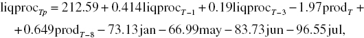
In this book, empirical linear econometric model is going to be the tool used for forecast estimation of a small-sized enterprise’s financial liquidity during a T period. A relative measure of liquidity (liqproc), which is described by the following econometric model 5.12, will be the forecasted variable:

In model 5.12, there are23: liqproc – observations of the explanatory variable, which represent a relative measure of the financial liquidity in the company REX, calculated using Equation 5.2; liqproc−1, liqproc−3 – volumes of the variable liqproc delayed by 1 and 3 months; prod – the value of ready-made production in a t month; prod−8 – the value of ready-made production delayed by 8 months; jan, may, jun, jul – the dummy variables, taking the value of 1 in the indicated month and the value of 0 in the remaining months – where the variables for January (jan), May (may), June (jun), and July (jul) turned out to be statistically significant; ulpr – represents equation’s residuals; t – the number of statistical observations (t = 1, …, 132).
Model 5.12 shows that the relative liquidity described here is characterized by autoregressions of the first and the third order that are sequential in nature. Impact of the current and the delayed by eight months values of the finished ready-made production is negative, thus it causes reduction of the relative liquidity’s level. The dummy variables appearing in the equation indicate that in January, May, June, and in July, the value of the liquidity measure was less than the value of corresponding parameter estimations, in comparison with the so-called systematic component of the model.
Considering the type of statistical data, the stochastic characteristics indicate good description accuracy of the variable liqproc described by model 5.12. It is illustrated by Figure 5.18. All explanatory variables can be considered statistically significant on the significance level γ ≤ 0.047. In the model, there is no autocorrelation of the random component, which is evidenced by the empirical Durbin–Watson statistic (DW5 = 1.987). As such, this model can be considered a good analytical instrument and a forecasting tool of the company’s liquidity.

Figure 5.18 The actual and the theoretical monthly values of the variable liqproc (calculated on the basis of model 5.12) during the years 1996–2006.
Further in this work, forecasts of the considered variable characterizing financial liquidity in the company REX were estimated. These forecasts will be short termed in nature and will involve the 12 months of the year 2007.
Forecasts of relative liquidity (liqprocTp) were estimated, assuming limitations of the ready-made production volumes planned for 2007, implemented during successive months of that year. Based on this assumption, the following forecasts are generated automatically. The principle of sequential forecasting is applied here, due to the delayed variables liqprocT−1, liqprocT−3, and prodT−8. The volumes of the dummy seasonal variables are known automatically. Results of the calculations done using the GRETL package are presented in Table 5.8 and in Figure 5.19.
Table 5.8 Monthly forecasts of ready-made production for the year 2007, in thousands PLN.
| Forecasted period | Forecast (prodTp) | Average prediction error | Forecast range at a confidence level of 95% |
| 2007:01 | 61.2 | 26.03 | 9.6 ÷ 112.7 |
| 2007:02 | 65.1 | 26.03 | 13.5 ÷ 116.6 |
| 2007:03 | 53.6 | 26.03 | 2.0 ÷ 105.1 |
| 2007:04 | 45.8 | 26.41 | −6.5 ÷ 98.1 |
| 2007:05 | 63.6 | 26.41 | 11.3 ÷ 115.9 |
| 2007:06 | 41.3 | 26.41 | −11.0 ÷ 93.6 |
| 2007:07 | 25.7 | 26.42 | −26.7 ÷ 78.0 |
| 2007:08 | 44.3 | 26.42 | −8.0 ÷ 96.6 |
| 2007:09 | 70.3 | 26.42 | 18.0 ÷ 122.6 |
| 2007:10 | 38.1 | 26.42 | −14.2 ÷ 90.5 |
| 2007:11 | 33.2 | 26.42 | −19.1 ÷ 85.6 |
| 2007:12 | 55.0 | 27.37 | 0.8 ÷ 109.2 |

Figure 5.19 Monthly forecasts of ready-made production for the year 2007, in thousands PLN.
Source: Table 5.8 (generated using the GRETL package).
The estimated forecasts are characterized by a precision sufficient for the purposes of current management of a small-sized company. They allow appropriate preparation of the projects assumed during the forecasted period, which comprise obligations to various contracting partners.
It is the responsibility of modern economics to offer simple tools supporting decision-making to business practices, including the persons managing variously-sized enterprises. The simple statistic method of financial liquidity analysis, which is presented in this book, can be widely and easily used in every manufacturing company. It requires, however, creation of an appropriate system for collecting relevant data about the results of the company’s past activity. Collection of such important statistical data small-sized enterprises can occur in only when their owners (managers) will recognize and appreciate all significant benefits of possessing such data, especially economic and management benefits.
We are going to estimate the prognoses of liqprocTp for 12 successive months of 2007. To do so, a predictor emerging the empirical Equation 5.12 is going to be used:
The condition for a forecast estimation of liqprocTp for successive future time-periods is possession of information about future values of ready-made production (prodT). Thus, it will be necessary to have a predictor, which allows forecast estimation (prodTp). As such, an autoregressive-trendy equation describing the volatility mechanism of ready-made production was constructed. It enabled construction of a predictor in the following form:
The prognoses of ready-made production for successive 12 months of 1007 were estimated. Estimation results are presented in Table 5.8.
Forecast estimations of ready-made production for successive months of 2007 (prodTp) are illustrated in Figure 5.19. Large average prediction errors for each of the prognoses (VT) as well as high relative prediction errors (![]() ) draw attention. They result from specificity of small-sized enterprise’s statistical data. Large amplitude of fluctuations in the time-series of small-sized enterprises results in a significant share of the random variable. Consequently, it is difficult to obtain empirical equations with a high value of R2. In our case, forecast values of prodTp play an important role as the expected values at the autoregressive values of explanatory variables and of the time variable T in the predictor equation 5.14. The obtained forecasts of ready-made production allow estimation of a small-sized enterprise’s financial liquidity forecasts, expressed by the variable liqprocTp, in the form of a forecast.
) draw attention. They result from specificity of small-sized enterprise’s statistical data. Large amplitude of fluctuations in the time-series of small-sized enterprises results in a significant share of the random variable. Consequently, it is difficult to obtain empirical equations with a high value of R2. In our case, forecast values of prodTp play an important role as the expected values at the autoregressive values of explanatory variables and of the time variable T in the predictor equation 5.14. The obtained forecasts of ready-made production allow estimation of a small-sized enterprise’s financial liquidity forecasts, expressed by the variable liqprocTp, in the form of a forecast.
Forecasts of financial liquidity liqprocTp were estimated using predictor 5.13 (Figure 5.20). Forecast estimations are presented in Table 5.9.

Figure 5.20 Forecast estimations of relative liquidity (liqprocTp) and forecast rages at a confidence level of 95% t (115, 0.025) = 1.981.
Source: Table 5.9 (generated using the GRETL package).
Table 5.9 Monthly forecast estimations of relative liquidity (liqprocTp), of average prediction errors (VT) and of relative prediction errors (![]() ) as well as forecast ranges at a confidence level of 95% t (115, 0.025) = 1.981.
) as well as forecast ranges at a confidence level of 95% t (115, 0.025) = 1.981.
| Forecasted period | Forecast (liqprocTp) | Average prediction error (VT) | Relative prediction error ( |
Forecast range at a confidence level of 95% |
| 2007:01 | 259.91 | 68.2 | 26.2 | 124.75 ÷ 395.07 |
| 2007:02 | 365.37 | 73.9 | 20.2 | 219.07 ÷ 511.67 |
| 2007:03 | 345.77 | 74.8 | 21.6 | 197.64 ÷ 493.90 |
| 2007:04 | 334.68 | 76.9 | 23.0 | 182.39 ÷ 486.96 |
| 2007:05 | 298.80 | 77.9 | 26.1 | 144.44 ÷ 453.17 |
| 2007:06 | 283.51 | 78.3 | 27.6 | 128.42 ÷ 438.59 |
| 2007:07 | 268.49 | 78.6 | 29.3 | 112.87 ÷ 424.11 |
| 2007:08 | 342.56 | 78.7 | 23.0 | 186.61 ÷ 498.51 |
| 2007:09 | 309.70 | 78.8 | 25.4 | 153.59 ÷ 465.81 |
| 2007:10 | 359.20 | 78.9 | 22.0 | 202.00 ÷ 515.40 |
| 2007:11 | 395.98 | 78.9 | 19.9 | 239.73 ÷ 552.24 |
| 2007:12 | 356.96 | 78.9 | 22.1 | 200.67 ÷ 513.25 |
In case of forecast estimation of a small-sized enterprise’s financial liquidity, a relative limiting error at a level 15–20% is admissible. The estimated forecasts of liqprocTp are characterized by adequate precision – in terms of decisional needs in a small-sized enterprise. They indicate that during the entire 2007 high level of the company’s financial liquidity can be expected. It does not mean that this liquidity will emerge spontaneously, or almost automatically. It means that the system of product manufacturing quality as well as the principles of debt recovery, both recently used in the company, should be maintained. It is also going to be necessary to monitor the company’s actual financial liquidity during successive months of 2007. Possible excessive negative derogation of the actual liquidity, compared to the forecasted liquidity, will require an adequate reaction on the part of the company’s management.
An approach enterprise’s financial liquidity24 – different from those so far presented in literature – makes it possible to obtain more precise results. It allows a detailed insight into the present and into the history of the changes in liquidity. It increases security during a possible credit granting for the company. Particularly, simultaneous examination of the liquidity, using the three research tools proposed here, can effectively increase the description precision of liquidity, and thus enhance the company’s competitive strength. Having the time series indicated in this work, allows construction of econometric models describing financial liquidity. Besides its diagnostic properties, such a model can also be used, to estimate shortly-timed liquidity forecasts. Widespread availability of GRETL (http://gretl.sourceforge.net/) provides an opportunity of sequential correcting the forecasts, performed along with flow of information, due to lapsing of time.