
4
An empirical econometric model of a small-sized enterprise1
4.1 Specification of a small-sized enterprise’s econometric model
The mechanism linking important economic variables of a small-sized enterprise has many features that are common with a structure of a large- or medium-sized company. There are, however, more differences than similarities, which can be noticed while analyzing Figure 4.1.

Figure 4.1 Economic interdependencies in a small-sized enterprise.
Source: Wiśniewski, J. W. (2003): An econometric model of a small-sized enterprise, Chapter 2.
There is a significant difference in the perception of reality within a small-sized company, in comparison to a large-sized one – the domination of a short time-horizon. In a small business entity, monthly vision prevails over the annual one. A quarter, in a small-sized company, is a period of a longer perspective, than a year in a large-sized company. Therefore, for example, perception of a small-sized company’s production is divided into three parts. Specificity of a small-sized manufacturing enterprise requires distinction of three concepts: manufacture of ready-made production, the amount of the sales income, and the cash inflows obtained from the sales. Between those concepts, each of which represents a category of economic production, there is a time interval which is significant for a small-sized business entity. The company can manufacture and store in confined spaces the goods that were not sold. Even if formally there is a sale expressed in the sales income resultant from invoicing the goods, still, it can indicate a beginning of hardships for the company. As a result of manufacturing the goods and post-delivery invoicing the recipients, numerous liabilities on the part of the company follow: to the suppliers of raw materials and substances, to the workers, public and legal obligations, and many others. If manufacturing the goods and their delivery to customers do not result in an income of respective amounts of money, and if the company cannot – using other sources of financing – pay off its obligations, in an extreme case, it can lead to bankruptcy of a small business entity.
Figure 4.1, thus, distinguishes the cash inflows as a result of delivering the goods, formally reflected by the sales income being the sum of the amounts on the invoices issued during a given period of time. Sales income can be generated if the finished goods, in the diagram represented by the ready-made production, were manufactured in advance. The company’s marketing potential2 is an important factor impacting the sales income. Production size, understood as the volume of the ready-made goods prepared for sale, is conditioned by some conventional factors, among which labor resources and fixed assets play a dominant role. It may happen that production is subject to influence of other conditions, some of which may be production specialization, product properties, and others. Labor efficiency plays a significant role in shaping the size of production.
Effectiveness of major tangible factors determines the enterprise’s competitive strength. A company characterized by high labor productivity, or by higher productivity of the noncurrent assets, has a chance for lower production costs, which makes that company stronger in the area of price competition. Labor efficiency, here understood as team efficiency,3 is in a feedback relation with the wage, provided that the motivational system is properly constructed. Efficiency stays under the influence of various numerous factors, among which technical progress and production specialization were indicated in the mechanism of linkage.
Wages – being subject to influence of labor efficiency – depend on many different factors, among which the following deserve to be highlighted: the autonomous process of a wage increase4 as well as the company’s financial situation, largely determined by the cash inflows. The wages in the company, in turn, affect the labor resources, both, in their quantitative as well as qualitative characteristics.
The volume and the quality of labor resources depend on the characteristics of the noncurrent assets.5 The labor supply resultant from a demographic situation also plays an important role.
Fixed assets, on one side, result from the capital investments realized by the company and, on the other, result from consumption of the assets’ components, making it necessary to carry out replacement investments. Investment opportunities, to a large extent, are conditioned by the company’s financial situation, which largely depends on the sizes of the cash inflows.
4.2 The structural form of a small-sized enterprise’s econometric model
4.2.1 The model’s total interdependent variables
The multiple-equation econometric model will describe economic interdependencies of a small manufacturing enterprise belonging to a publishing and printing sector.6 It belongs to a business category, which allows simplified accounting in the form of the so-called revenue and expense ledger. At the same time, the company has been liable for the tax on goods and services (VAT), ever since its introduction in Poland. Since 1991, the company has been operating on a highly competitive market. The study covers the years 1996–2000. This period, in which the company was operating in its own facility connected with a property constituting its mortgage ownership,7 can be described as relatively stabilized. As such, it is a time interval in which stability of the company’s headquarters was guaranteed, thus the owners had favorable conditions for development through appropriate investments.
Figure 4.1 constitutes the basis for defining the variables of a small-sized enterprise’s econometric model. Equivalent variables discussed in Section 4.1, which represent the categories under the influence of at least one other element, will form a set of endogenous variables of an econometric model composed of many stochastic equations.
This means that the following will be the total interdependent variables of the econometric model:
- CASH – the amount of the cash inflows during a period t, in thousands PLN8;
- SBRUT – gross sales income during a period t, in thousands PLN;
- PROD – the value of ready-made production (in sale prices) during a period t, in thousands PLN;
- EMP – the number of employees calculated in full-time employment during a period t (number of people)9;
- FIXAS – the initial value of the tangible fixed assets in use during a period t, excluding buildings and constructions, in thousands PLN;
- EEFEMP – labor efficiency as a quotient of the ready-made production’s value and the number of employees (PROD/EMP), in thousands PLN per 1 employee, during a period t;
- SAL – net salary paid to the company’s employees for their work during a period t, in thousands PLN;
- APAY – the average monthly wage paid to the employees during a period t (in PLN);
- INV – the value of capital expenditures during a period t (in net purchasing prices10), in thousands PLN.
Some of the elements described in Figure 4.1 have been additionally expressed by other variables, which will belong to the group of the total interdependent variables. These are as follows:
- SALPR – effectiveness of the net salary expressed by a quotient of the ready-made production and the net salary (PROD/SAL), in production PLN per 1 PLN of the net salary;
- EFSAL – effectiveness of the net salary calculated as a ratio of the sales income to the sum of net salaries (SNET/SAL), in PLN income per 1 PLN of the net salary;
- ESC – effectiveness of the net salary as a relation of the cash inflows to the sum of the net salaries (CASH/SAL), in PLN inflows per 1 PLN of the net salary11;
- MACH – the value of equipment and machinery (its initial value) in thousands PLN.12
Figure 4.1 shows direct feedback between the wage and the labor efficiency. In the econometric model, this feedback will be manifested by the following hypothetical linkage:

What is more, at least three closed cycles of links between the total interdependent variables13 occur in the econometric model. The first one has the following form:

The second of those closed cycles linking the total interdependent variables is as follows:

Finally, the third indirect feedback takes on the following form:

Indirect and direct feedback in the hypothetical model, both determine its affiliation with a class of interdependent systems. In this model, it is also possible to predict occurrence of the so-called detached equations, which are characterized by the fact that only the predetermined variables are those equations’ explanatory variables.
4.2.2 The model’s predetermined variables
The first group of the variables forming a set of econometric model’s predetermined variables is composed of exogenous variables. They represent the categories in Figure 4.1, which have impact on other elements of the system, but are not dependent on the rest of its categories. The second group, constituting a fraction of the set of predetermined variables, is composed of time-delayed endogenous variables.14
In the econometric modeling, the so-called methodology of dynamic consistency models15 will be used. Accordingly, application of autoregressive solutions in various stochastic equations will be attempted. This means that each of the endogenous variables potentially will appear in the group of predetermined variables.
The following will be the model’s exogenous variables:
- DEPR – the value of the tangible fixed assets’ depreciation during a period t, in thousands PLN;
- AMPL – the quotient of the net payroll during a period t and the amount of the fixed assets’ depreciation (SAL/DEPR), in PLN (of the wages) per 1 PLN of depreciation;
- RAN – the number of the product assortments for sale (the mean during a period t), as occurring on the price list;
- MARK – the dummy variable, distinguishing the periods in which the company’s representatives actively attended fairs,16 whereas RAN = 1 in quarters (in months) of fair participation and RAN = 0 in the remaining periods;
- TAM – technical devices as a ratio of the initial value of machinery and equipment to the number of employees (MACH/LAB), in thousands PLN of machinery and equipment’s value per 1 employee;
- TAL – technical devices as a ratio of the initial value of the tangible fixed assets in use to the number of employees (FIXAS/LAB), in thousands PLN per 1 employee;
- FIXD – initial value of tangible fixed assets in use per one unit of depreciation costs during a period t (FIXAS/DEPR),17 in PLN per 1 PLN of depreciation costs;
- TIME – the time variable, assuming the values 1, …, 84 in case of monthly data and 1, …, 28 in quarterly time series.
In the econometric modeling, exogenous variables with their adequate time delays will also occur. In the model, they will also belong to a category of predetermined variables.
4.2.3 Structural-form’s equations of a small-sized enterprise’s econometric model
In our considerations, the system of interdependent stochastic equations is formed by18


Occurrence of many time-delayed variables in the model causes a modeling impediment for two reasons. First, the delays decrease the number of statistical observations – in this case, by a maximum of m number of series components19 (in quarters or months). What is more, taking those delays into account increases the number of structural parameters in the structural-form’s equations, especially in the equations of a reduced form. In extreme cases, this leads to a lack of a positive number of the degrees of freedom, which prevents estimation of their parameters.
The study examined some delays, in monthly data by m = 12 periods and delays for quarterly series by m = 4. Consequently, in the reduced-form’s equations, which take into account all the delayed variables, after reducing the number of observations by m (12 or 14), the difference between the number of statistical observations (n = 84 monthly or n = 28 quarterly) and the number of structural parameters became negative. Such situation prevents using the ordinary least square (OLS) method to estimate the parameters of the structural-form’s equations. Therefore, it was necessary to experiment on the structural-form’s equations using the OLS method. The purpose of this procedure was to eliminate from the equations all the variables that are statistically insignificant, that is, the variables for which empirical statistics of a t-Student have turned out to be particularly small,20 at a particularly high risk of a type I error. With these preparatory proceedings, it was possible to use the 2LS method for each of the structural-form’s interdependent equations. In the subsequent iterations, statistically insignificant variables were eliminated from each empirical equation. As a result of this procedure, the reduced-form of the model was also modified. The empirical equations presented below result from the examination proceedings described here. This book is going to present empirical results of econometric modeling, which are based on monthly data. This type of results is used for current management decision-making in small enterprises.
4.3 Equation of the cash inflows
An empirical equation, constructed on the basis of monthly data, has the following form:

In Equation 4.12, there are two explanatory variables with relatively small empirical values of the t-Student statistics.21 They allow an inference that the variables CASH−11 and TIME can be deemed significant at a significance level of γ ≈ 0.15. These variables, however, were left in the equation due to their epistemic qualities. Figure 4.2 showed the actual and the theoretical monthly amounts of the cash inflows as well as the residuals calculated on the basis of Equation 4.12, while Figure 4.3 presented distribution of the residuals of Equation 4.12.

Figure 4.2 The actual and the theoretical monthly amounts of the cash inflows as well as the residuals calculated on the basis of Equation 4.12.

Figure 4.3 Distribution of the residuals of Equation 4.12.
It can be assumed that Equation 4.12 quite accurately describes the principles of monthly cash inflows, since around 83.4% of their volatility results from the impact of the variables CASH−11, SBRUT, SBRUT−2, SBRUT−4, SBRUT−10, and TIME. The actual monthly amounts of cash inflows differ from those calculated on the basis of Equation 4.12, on average, by 17.9 thousands PLN, which represents 16.16% of the average monthly value of the variable CASH during the period of 1996–2002. At the same time, an empirical size of the Durbin–Watson (DW) statistic = 2.185 indicates22 that there are no grounds for rejection of the null hypothesis about the lack of the first-order autocorrelation of the random component.
Autoregression of the 11th order, in the statistical sense, is weak. The revenues obtained 11 months earlier, in the amount of 1000 PLN, entail an increase in the current inflows by around 104 PLN.23 Also, the time variable in Equation 4.12 belongs to those relatively weak statistically. The upward linear trend indicates an increase in the cash inflows, independently of the other explanatory variables. It can be inferred that the enterprise’s receivables collection system has been improving regularly. This can result, inter alia, from elimination of unreliable trading partners as well as from systematic contacts and work with the clients. It is facilitated through the use of the so-called direct marketing combined with rewarding the sales representatives solely on the basis of the amounts of money obtained from the supported sales network.
Sales income, that is the sales validated by invoices, are major source of cash inflows. For 1 thousand PLN invoiced in a current month,24 the company gains, on average, around 522 PLN in cash. Invoicing a 1000 PLN prior to 2 months results in current inflows bringing, on average, 135 PLN. Lastly, a 1000 PLN invoiced prior to 4 months results in current cash inflows in the amount of 174 PLN.
The variable SBRUT−10 has a negative impact on the current cash inflows. This dependence confirms that customers often rely on their guaranteed right to return a product by issuing a corrective invoice, which causes a decrease in the accounts receivable, and consequently a lack of adequate cash inflows.
A linear equation describing the mechanism of cash inflows’ formation has the following empirical form (in case of quarterly observations)25:

Figure 4.4 presents the company’s actual quarterly cash inflows, the theoretical values calculated using Equation 4.13, and the rests, that is, the differences between empirical and theoretical values.

Figure 4.4 The actual and theoretical27 quarterly values of the cash inflows and the residuals of Equation 4.13.
Equation 4.13 indicates that the quarterly amounts of cash inflows are characterized by a third-order autoregression. This autoregression shows that the company’s cash inflows from 3 quarters ago shape their current amount, wherein the relationship is negative. It allows a conclusion that the sums previously acquired from the receivers reduce current liabilities, and thereby reduce the current inflows.
The impact of the sales income’s size on the cash inflows, in quarterly terms, is both current as well as delayed by 1 quarter. Impact of the concurrent amounts resultant from invoicing customers on the variable CASH, expressed by a parameter estimation equal to 0.658, means that for every thousand of the sales income achieved in the quarter for which the invoices were issued, a sum of 658 PLN is obtained in the form of cash and/or a bank transfer to the company’s bank account. For 1 thousand PLN invoiced in a previous quarter, the company obtained, on average, 391 PLN of cash inflows. Each of the explanatory variables occurring in the empirical equation 4.13 is statistically significant at a low significance level of γ < 0.01. Figure 4.5 presented distribution of the residuals of Equation 4.13.

Figure 4.5 Distribution of the residuals of Equation 4.13.
The multiple-correlation coefficient squared indicates that 89.3% of the total volatility of the cash inflows is explained by the variables CASH−3, SBRUT i, SBRUT−1. Such result marks high description accuracy of the variable CASH for quarterly time series. Random fluctuations of the variable CASH are relatively small, since an estimated value of the standard residual deviation, equal to 36.8 thousands PLN, can be considered as small. It indicates that the theoretical values of the cash inflows, calculated using Equation 4.13, differ from the actual ones, on average, by 36.8 thousands PLN. The value of the DW2 statistic equal to almost 2 indicates that there is no first-order autocorrelation of the random component.
4.4 Equation of the sales income
An empirical equation describing monthly gross sales income has the following empirical form:
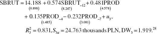
Equation 4.14 is characterized by good description accuracy of monthly gross sales income. Around 83.1% of SBRUT’s volatility is explained by an autoregression of the 12th order, the executed current value of ready-made production, and by ready-made production delayed by 4 and 7 months. Figure 4.6 shows this equation’s high fitting accuracy, when compared to the equations based on microeconomic monthly data. Figure 4.7 presented distribution of the residuals of Equation 4.14.

Figure 4.6 The actual monthly gross sales income, the theoretical values, and the residuals calculated on the basis of Equation 4.14.

Figure 4.7 Distribution of the residuals of Equation 4.14.
Equation 4.14 reveals repetitiveness of income every 12 months. This means that a sales income of a 1000 PLN achieved prior to 12 months entails current amounts of that income in about 574 PLN. A current value of ready-made production, in the amount of 1000 PLN, results in the sales income of 481 PLN. Ready-made production, in the amount of 1000 PLN prior to 4 months, has a current effect in the form of the sales income amounting to 135 PLN. The variable PROD−4 can be regarded as statistically significant,29 with a 6.95% risk of a type I error. Finally, negative autoregression of the seventh order confirms elimination of some of the expired ready-made goods from the sales, while the waiting period for their designation as waste paper, on average, lasts 7 months.
An empirical equation of the gross sales income, based on quarterly data, has the following form:

Explanatory variables of the equation are statistically significant at a significance level γ below 0.01. The empirical value of the Durbin–Watson statistic DW4 = 1.586 > du = 1.30 at a significance level of γ = 0.01, which allows a conclusion that in Equation 4.15 there is no first-order autocorrelation of the random component. Figure 4.8 illustrates the volatility of the actual and the theoretical values of the sales income as well as the residuals of Equation 2.3, while Figure 4.9 shows distribution of this equation’s residuals.
Figure 4.8 The actual quarterly values of the gross sales income, the theoretical values and the residuals calculated on the basis of Equation 4.15.

Figure 4.9 Distribution of the residuals of the empirical equation of the gross sales 4.15.
It is somewhat surprising that Equation 4.15 contains only the volume of the current ready-made production PROD as well as third-order and fourth-order autoregressions. In the empirical equation there was no RAN or MARK variables characterizing, on one hand, the variety and versatility of the trade offers, and on the other, participation in trade fairs, as a way of influencing the customers.
For each 1000 PLN of quarterly ready-made production, there is a gross sales income of about 843 PLN. This confirms the initial hypothesis about a necessary production in advance, where, in some cases, the goods await delivery to the client for a period longer than 3 months. Such situation results from a highly competitive market with a large amplitude of seasonal sale fluctuations.
Negative impact of the delayed by 3 quarters sales income on the current amounts obtained as a result of deliveries can, on one hand, result from the returns of some seasonal goods,30 while on the other, the goods lingering at the recipient’s cause his/her natural aversion for additional purchases. This mechanism forces the manufacturer to more accurately and precisely account for the size of the finished production to avoid returns or not to run out of the goods during a period of intensive purchases, as not to cause the supplier to be displaced by a competitor who is able to satisfy the demand on the market.
Positive interaction of the variable SBRUT−4 indicates repeatability of the sales every 4 quarters. This means that a sales income achieved by the end of 4 quarters, in the amount of 1000 PLN, generates its current amount of about 523 PLN.
4.5 Equations of ready-made production
An empirical equation describing the volatility mechanism of a monthly ready-made production has the following from:

Description accuracy of the formation mechanism of the monthly ready-made production values is significantly worse in comparison with Equations 4.12 and 4.14. This is due to the specificity of manufacturing for store, which entails production of semifinished goods that were not included in the ready-made production account. This principle is visible in Figure 4.10, which shows the seasonality of the ready-made production’s dynamics, on a monthly basis.32 Therefore, at a large amplitude of the variable PROD’s seasonal fluctuations, the degree of explanation of the ready-made production’s volatility at a level of 65% can be considered as satisfactory. Figure 4.11 presented empirical values of monthly ready-made production, the theoretical values, and the residuals, calculated on the basis of Equation 4.16.

Figure 4.10 Monthly seasonal fluctuations of the ready-made production’s dynamics index, in the years 1996–2002.

Figure 4.11 Empirical values of monthly ready-made production, the theoretical values and the residuals, calculated on the basis of Equation 4.16.
The explanatory variables appearing in Equation 4.16 are statistically significant on a significance level ranging from γ = 0.0766 (for EMP−8) to less than γ = 0.001 (for PROD). Autoregressions of the 4th and the 12th order signify repetitiveness of the production scale every 12 months33 as well as its correction every 4 months34 by the amount of about 175 PLN.
The current and the delayed by 8 months employment, both are stimulators of the ready-made production’s size. An increase in employment by one person allows a simultaneous increase in the ready-made production’s value, on average, by 2894 PLN. Employment growth by one person, prior to 8 months, generates a current production-effect in the amount of about 2918 PLN, which means that the period of employee’s adaptation to his/her work position needs to pass, ultimately resulting in his/her improved efficiency.
In the equation discussed here, the variable FIXAS has been supplanted by a type of its mutation in the form of FIXAS delayed by 2 and 12 months. An increase in the initial value of the tangible fixed assets in use by 1 PLN per 1 PLN of depreciation costs, prior to 2 months, causes an increase in the current ready-made production’s value, on average, by about 616 PLN. Along with an increase in the variable FIXAS’s value, prior to 12 months, by 1 PLN, there is a current decline in the ready-made production’s value, on average, by 506 PLN. The downward trend of the ready-made production, as evidenced by a negative assessment of the parameter along the variable TIME, draws attention. The company follows a deceleration of its production activity, due to an unfavorable entrepreneurial situation, especially owning to the law regulations and law enforcement in the past period. Finally, the variable RAN positively influences the value of the ready-made production. An increase in the number of manufactured assortments by 1 allows an increase in the ready-made production, on average, by 2162 PLN.
An empirical equation of the finished production’s value constructed using quarterly data has the following form:

Among the explanatory variables, the variable FIXAS is statistically significant at a significance level of γ = 0.0818. All other explanatory variables are statistically significant at 0.01 < γ < 0.07. Explanatory variables included in Equation 4.17 explain 87.6% of the finished production’s quarterly volatility. The actual values of the finished production, calculated on the basis of Equation 4.17, differ from its theoretical ones, on average, by 40.680 thousands PLN.
Commutativity of the signs of the coefficients by the variables forming autoregressive dependencies (PROD−2, PROD−3, PROD−4) result from the process of creating inventories of finished goods. During the periods of low-intensity sales, semifinished goods, which can be quickly converted into finished goods and delivered to clients, are manufactured and stored. This way, the company’s manufacturing potential is used more rhythmically.
The negative sign of the assessment of the structural parameter by the variable FIXAS can be surprising. Based on that, it cannot be inferred that an increase in the value of the company’s noncurrent assets causes a decrease in the ready-made production. However, it follows that the accumulated noncurrent assets are not fully utilized. The resources gathered depend on the demand during the periods of the so-called production peak. This allows avoidance of outsourcing some of the tasks to outside subcontractors, who limit the company’s independence and generate higher costs.
The variable FIXD, which expresses a general relation of the noncurrent assets’ initial value to the depreciation costs in a given period, contains complementary information about the impact of the noncurrent assets on production performance. A decrease in the FIXAS rate indicates a renewal of the noncurrent assets, while an increase in this variable’s value indicates aging of the manufacturing potential. Negative signs of the parameters at FIXAS and FIXAS−3 confirm a positive impact of new36 machinery and equipment on the size of the manufactured production. A positive sign of the assessment of the variable FIXD−2 can be interpreted as information about a production increase influenced by an increasing value of the considered variable, with a half-year delay. This may be a consequence of a second quarter period, which is necessary for the employees to adapt to new machinery (equipment), after expiration of which they acquire proper equipment operating efficiency.
Finally, the time variable provides information about a positive trend of manufactured production, followed by an independent increase in the finished production’s quarterly value, on average, by 30.227 thousands PLN. It can be interpreted as a result of a neutral technological and organizational progress, which occurred in the company ( Figure 4.12).

Figure 4.12 The actual quarterly values of finished production, the theoretical values and the residuals, calculated on the basis of Equation 4.17.
4.6 Equation of labor efficiency
The formation mechanism of monthly team-labor efficiency is much more complicated. An empirical equation describing a monthly volatility of the variable WP has the following form:

In the empirical equation 4.18, autoregressive interdependencies of the 4th, 6th, 8th, 10th, and 11th order are significant. Negative signs of the assessments of the structural parameters by the efficiency volumes that are delayed by 4, 6, 8, and 10 months indicate the mechanism’s commutativity. On the other hand, an increase in labor productivity by 1000 PLN per 1 employee, prior to 11 months, results in an increase in the variable EFEMP’s current value, on average, by 248 PLN per 1 employee. Figure 4.13 presented the actual monthly values of team-labor efficiency, the theoretical values, and the residuals calculated on the basis of Equation 4.18.

Figure 4.13 The actual monthly values of team-labor efficiency, the theoretical values, and the residuals calculated on the basis of Equation 4.18.
The average monthly net pay is an important efficiency stimulator.38 An increase in the average net pay by 1 PLN per 1 employee results in an increase in labor efficiency, in this respect, on average, by 8.77 PLN per 1 employee. The average monthly net wages delayed by 6 and 10 months positively influence labor efficiency as well. The average monthly net wages delayed by 5 and 11 months inhibit labor efficiency. However, the sum of the parameter estimations along the current SRPL and the delayed SRPLs is distinctly positive, which indicates a positive influence of the average wages on labor efficiency. This confirms the thesis about the company’s properly constructed motivational wage-system.
Technical devices (TAL) affect labor efficiency with the delays of 2, 3, and 4 months. The delays in TAL’s impact on the labor efficiency result from an imperative period of human adaptation to new technology. The sum of the coefficients for the variables TAL−2, TAL−3, and TAL−4 is positive, which signifies a final positive impact of the technical devices’ increase on labor efficiency. At the same time, the negative linear trend of labor efficiency suggests negative technical-organizational changes, detrimental to human-labor effectiveness.
Next empirical equation belongs to the pair expressing a feedback between the team efficiency and the average pay. It describes the quarterly formation mechanism of labor efficiency in the following form:
Equation 4.19 indicates that an increase in the average net pay by 1 PLN net per 1 employee is followed by an increase in the team-labor efficiency, on average, by 5.6 PLN per 1 employee. This means that the net pay is a significant stimulator of labor efficiency. It allows a conclusion about a properly constructed motivational system within the company. Simultaneously, there is a second-order autoregression of the team-labor efficiency. A negative sign of the coefficient by the variable EFEMP−2 indicates alternation of increases and decreases of the EFEMP’s value every two quarters. An increase in the variable EFEMP by 1 thousand PLN per 1 employee, prior to 2 quarters, is followed by a current decrease in efficiency, on average, by 518 PLN per 1 employee. An average increase by 518 PLN per 1 employee is a response to a 1 thousand PLN per 1 employee decline in the team-labor efficiency prior to 2 quarters. There is an effect of producing semifinished goods during the periods of sale declines to prepare a necessary inventory that would allow satisfaction of the demand on the market during a period of the so-called peak season.
Description accuracy of the quarterly mechanism of team-labor efficiency is significantly worse than in case of other interdependent variables, which is illustrated in Figure 4.14. Only 69.4% of the labor efficiency’s volatility is explained by autoregression of the second order as well as by an average monthly pay in a given quarter.

Figure 4.14 The actual values of quarterly team-labor efficiency, its theoretical values, and the residuals calculated on the basis of Equation 4.19.
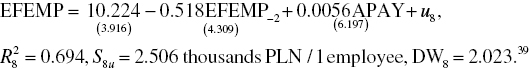
4.7 Equations of the average wage
An empirical equation describing formation of the average monthly net wage, based on monthly time series, has the following form:

Figure 4.15 presented the actual average monthly net wages, their theoretical values, and the residuals, calculated on the basis of Equation 4.20. Likewise, in the equation describing APAY, feedback between the average net wage and the team-labor efficiency is confirmed, based on monthly time series. The variable EFEMP is statistically significant in Equation 4.20. An increase in monthly labor efficiency by 1 thousand PLN per 1 employee results in a simultaneous increase in the average net wage, roughly, by net 20.7 PLN per 1 employee. At the same time, there are negative impacts of the labor efficiency amounts delayed by 2 and 12 months on the current average net pay. This means that due to seasonal declines in labor efficiency, caused by production of semifinished inventories, employees are paid accordingly to their labor input. Thus, a decrease in labor efficiency, prior to 7 and 12 months, results in a current increase in the average net wage, due to the employees’ significant input into creation of grounds for future ready-made production.

Figure 4.15 The actual average monthly net wages, their theoretical values and the residuals, calculated on the basis of Equation 4.20.
The variable APAY, in a system of monthly observations, is characterized by autoregressions of the 1st, 6th, and 12th order. This signifies stabilization of a part of the standard net wage.41 An increase in the average net wage by 100 PLN per 1 employee in a previous month causes its current rise by about 45.28% PLN per 1 employee. The effects of similar wage raises prior to 7 and 12 months are lower and, respectively, equal to net 21.28 PLN and 23.13 PLN per 1 employee.
Description accuracy of the average net wage’s mechanism, based on monthly time series, is relatively high, since the explanatory variables of Equation 2.10 explain 90.6% of the variable APAY’s volatility. Also, S5u = 62.21 PLN per 1 employee confirms the above observation, because the theoretical values of the average net wage, calculated on the basis of Equation 4.20, are different from the actual ones, on average, by ±62.21 PLN per 1 employee, which represents 8.2% of the variable APAY’s average value in the years 1996–2002.
An empirical equation describing formation of the average monthly net wage, based on quarterly time series, has the following form:

The mechanism of the average monthly net pay is characterized by high description accuracy, since the explanatory variables of Equation 4.21 explain 94.0% of its volatility. High adherence precision of the theoretical values of the average pay in subsequent quarters in the years 1996–2002 is confirmed by Figure 4.16.
Figure 4.16 The actual average monthly net pay, the theoretical values and the residuals calculated on the basis of Equation 4.21.
Confirmation of a feedback between the average wage and the team-labor efficiency is economically important information contained within Equation 4.21. An increase in the average monthly net wage, on average, by 56.8 PLN per 1 employee, in a simultaneous quarter, occurs along with an increase in EFEMP by 1 thousand PLN per 1 employee. A negative assessment of the structural parameter at the variable EFEMP−4 indicates that every 4 quarters, correction of the average monthly pay occurs as a result of a significant arrhythmicity, especially in labor efficiency.
Autoregression of the fourth order is an important principle of the average monthly net pay’s quarterly volatility. This indicates consolidation of the wage level, as a company’s rule in force. An increase in the average monthly net pay by 100 PLN per 1 employee prior to 4 quarters results in an increase in the current monthly net wage by 73.4 PLN per 1 employee. Despite this fixed mechanism of the average wage increase, the motivational principle of determining a significant part of the wage still functions.
4.8 Equations of the net payroll
An empirical equation of monthly net payroll has the following form:

Formation mechanism of the enterprise’s monthly net payroll has many analogies compared to the equation describing a quarterly wage mechanism. Explanatory variables included in the empirical Equation 4.22 explain 89.5% of the payroll’s total volatility. The theoretical values of the variable SAL, calculated on the basis of Equation 4.22, are different from those observed, on average, by 1246 PLN, which represents 8.55% of the average monthly payroll in the years 1996–2002. It is illustrated by Figure 4.17.

Figure 4.17 The actual monthly values of the net payroll, the theoretical values and the residuals calculated on the basis of Equation 4.22.
Autoregressions of the 1st and the 11th order delimit an important part of the monthly payroll’s amount. An increase in the amount of this payroll by 1000 PLN in a previous month causes an increase in the variable SAL’s current value, on average, by 737 PLN. In contrast, the same increase in the discussed here payroll, prior to 11 months, results in a current increase in the net payroll in the amount of 133 PLN. Current cash inflows increased by a 1000 PLN cause a simultaneous increase in the net payroll, on average, by 12.26 PLN. The impact of the cash inflow amounts delayed by 2 months on the net payroll is negative, which signifies adequate fluctuations of the variable SAL.
Apart from regular payroll fluctuations, in each month of the year, its upward trend, in the nature of a fading curve, can be generally observed. Subsequent payroll increases are thus slower and become stabilized during the final observation periods.
The company’s net payroll depends, among other things, on its current financial situation conditioned by obtaining payments for the goods delivered to the customers. An empirical equation of the net payroll has the following from:

Equation 4.23 highly accurately explains the mechanism of quarterly fluctuations of the net payroll. Explanatory variables in this equation explain 89.8% of the variable SAL’s total volatility. At the same time, the theoretical values of the net payroll, calculated on the basis of the empirical Equation 4.23, differ from its actual ones in the previous quarters, on average, by 3896 PLN, which constitutes 8.9% of the company’s average quarterly net payroll amount. It is illustrated by Figure 4.18, which reveals a small discrepancy between the lines labeled as fitted and actual.

Figure 4.18 The actual quarterly values of the net payroll, the theoretical values, and the residuals calculated on the basis of Equation 4.23.
Autoregression of the first order is the first characteristic of the net payroll’s volatility. It shows that 1000 PLN increase in payroll in a previous quarter results in its current increase by around 707 PLN.
The volume of the cash inflows has a current and delayed by 1 and 12 quarters impact on the net payroll. This means that the financial situation, in terms of financial liquidity during the last half of the year, influences the size of the variable CASH. Generally, the company’s improved financial situation allows payout of higher net wages.
4.9 The employment equation45
An empirical equation describing the principles of formation of a monthly employment has the following from:

Figure 4.19 presented the actual monthly employment, theoretical employment, and the residuals calculated on the basis of Equation 4.24. The employment equation based on monthly data reveals the variable EMP’s strong autoregressive relations. Conclusion of an employment contract, especially for an indefinite time-period, makes the current status of employment a consequence of its level in previous months. Apparently, current employment status depends on the situation in a preceding month. Not all autoregressive relations are equally clear. The variable EMP−8 can be considered statistically significant when γ = 0.0696, while the variable EMP−2 – at a significance level of γ = 0.0391. These are not – as in the microeconomic equation based on monthly time series – very high risk-levels of a type I error.

Figure 4.19 The actual monthly employment, theoretical employment, and the residuals calculated on the basis of Equation 4.24.
The initial value of machinery and equipment, prior to 12 months, turns out to be employment stimulus. An increase in employment by 1 person in a current month results from an increase in machinery resources, prior to 12 months, by the amount of 61 thousands PLN, according to its net purchasing value. As such, complementary relations of employment and of the value of machinery and equipment are observed in the company.
The study has shown that the initial value of the tangible fixed assets in use47 FIXAS did not prove to be statistically significant, both in the employment equations describing a quarterly mechanism as well as monthly regularities. In practice, only ownership changes in terms of the variable MACH (with an adequate delay) cause necessary employment adjustments in the group of workers. Transportation means, in fact, are related to the sales representatives supporting the sales network. During the discussed period, the networks itself as well as the number of the sales representatives were stable. As a result, only the change of the so-called productive apparatus caused an adequate reaction of the variable EMP. Negative employment trends, both the quarterly as well as the annual ones, result from the process of substituting labor with capital, which occurred highly intensively in the period passed.
An equation describing employment formation, based on quarterly time series, has the following empirical from:

A dominant characteristic of the company’s employment volume is expressed by autoregressive relations up to and including the third order. There is a mechanism correcting employment, characterized by a negative assessment of the structural parameter by the variable EMP−2. It means that employment adjustment is made averagely every semester, involving reduction of the number of employees, on average, by one person annually.
Increasing the machinery resources results in an increase in employment, whiles the initial value of the machinery and equipment, prior to 4 quarters, is a statistically significant explanatory variable. Increasing the company’s machinery resources by around 23 thousands PLN triggers a response in the form of an employment increase by one person.
The quarterly volumes of employment are characterized by a linear trend. On average, a decrease in the number of employees, equal to a reduction of 1 employee each half of the year, occurs quarterly. This trend had become stronger at the end of the 1990s and lasted until the end of the observation period, as a reaction to inflexible employment opportunities in Poland and to rapidly rising costs of labor resultant from the actions undertaken by successive governments.
Description accuracy of the quarterly employment mechanism is moderate, since the explanatory variables included in Equation 4.25 explain 73.4% of the EMP’s overall volatility. There is no first-order autocorrelation of the random component in Equation 4.25, since DW14* = 1.743 > du = 1.53, at a significance level of γ = 0.01. Figure 4.20 illustrates the employment’s quarterly volatility and the results obtained from the empirical equation 4.25.
Figure 4.20 The actual employment, the theoretical employment volumes, and the residuals calculated on the basis of Equation 4.25 (quarterly data).
4.10 Equations of the fixed assets
An empirical equation describing the variable FIXAS, based on monthly data, has the following form:

Monthly fluctuations of the initial value of the fixed assets are caused by numerous explanatory variables. Autoregressive relations of the first, the seventh, and the eighth order play a significant role. The amounts of the money obtained earlier from the customers play an important role in shaping the noncurrent assets. The impact of the variables CASH−2 (while γ = 0.16), CASH−8 (for γ = 0.098), and CASH−12 (while γ = 0.0925) is relatively weak. Impact of the variable CASH with various delay periods confirms the earlier hypotheses as well as the calculation results obtained earlier on.
The impact of the variable SAL delayed by 6, 7, and 12 months on the size of the noncurrent assets is quite interesting. The sum of the positive parameter assessments by the variables SAL−7 and SAL−12 exceeds the negative value by the variable SAL−6. On the balance sheet, this means that an increase in the net payroll is followed by an increase in the initial value of the fixed assets. This can be interpreted as a reaction to the rising labor costs by further expansion of the noncurrent assets.
Equation 4.26 highly accurately explains the volatility of the variable FIXAS, which is illustrated by Figure 4.21. Explanatory variables of Equation 4.19 explain up to 99.1% of the overall volatility of the variable FIXAS. The theoretical values of the fixed assets, calculated on the basis of Equation 4.26, are different from their empirical values, on average, by 10472 PLN, which is 2.8% of their average monthly value in the years 1996–2002.

Figure 4.21 The actual initial values of the tangible fixed assets in use, the theoretical values, and the residuals calculated on the basis of Equation 4.26 (monthly).
A quarterly mechanism describing the initial value of the fixed assets is expressed by the following empirical equation:

Figure 4.22 presented the actual initial values of the fixed assets, the theoretical values, and the residuals calculated on the basis of Equation 4.27 (quarterly). The company’s quarterly fixed assets on the quarterly basis are characterized by a very strong autoregression of the first order. Additionally, the cash inflows from four quarters back positively influence its financial resources. This is due to application of the company’s principle of investing only own resources in the fixed assets. In fact, only a large inflow of cash prior to 4 quarters allows an increase in the noncurrent assets. An inflow of 100 thousands PLN prior to 4 quarters increased the current value of the variable FIXAS, on average, by 6540 PLN.

Figure 4.22 The actual initial values of the fixed assets, the theoretical values, and the residuals calculated on the basis of Equation 4.27 (quarterly).
Bank credit is too expensive for the company. Moreover, the procedures involving obtaining external sources of financing the business activity and development, for a small-sized company, are too complicated and require excessive security measures. The whole complexity of using a credit deters the company’s owner from applying to any of the financial institutions granting credits. As such, development opportunities of a small-sized company are significantly limited.
Equation 4.27 highly accurately describes volatility of the fixed assets, since autoregression and the cash inflows obtained prior to 4 quarters explain 98.4% of the total volatility of FIXAS. The theoretical values of the fixed assets, calculated on the basis of Equation 4.27, differ from their actual values, on average, by 13.716 thousands PLN, which constitutes 3.69% of the average value of FIXAS in the period between 1996 and 2002. In the equation, there is also a first-order autocorrelation of the random component, since DW16* = 1.410 > du = 1.20, at a significance level of γ = 0.01.
Next equation explains a quarterly mechanism48 of the machinery and equipment’s volatility. It has the following form:

Figure 4.23 presented the actual initial values of machinery and equipment, the theoretical values, and the residuals calculated on the basis of Equation 4.28 (quarterly). The value of machinery and equipment is subject only to an autoregressive dependence of the first order, which explains up to 95.6% of its total quarterly volatility. There was no impact of the variable CASH with any delay.

Figure 4.23 The actual initial values of machinery and equipment, the theoretical values and the residuals calculated on the basis of Equation 4.28 (quarterly).
An empirical equation explaining the mechanism of machinery and equipment’s volatility has the following form:
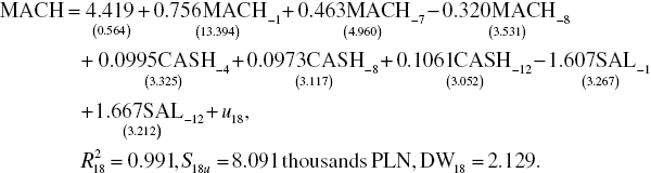
Figure 4.24 presented the actual initial values of machinery and equipment, the theoretical vales, and the residuals calculated on the basis of Equation 4.29 (monthly). In Equation 4.29, some analogies to the volatility mechanism of the total value of the fixed assets can be seen. It results from the fact that the variable MACH is a dominant component of the variable FIXAS, which, in the following years, is about 77%. All observations and explanations included in the characteristic of Equation 4.19 can be referred to in this case as well. A significant role of the cash inflows (CASH) with various delay periods in the formation of the machinery and equipment’s volatility (MACH) can also be recognized.

Figure 4.24 The actual initial values of machinery and equipment, the theoretical vales, and the residuals calculated on the basis of Equation 4.29 (monthly).
Next four empirical equations describe the mechanisms of the investments aimed at expansion of the total amount of fixed assets as well as on expansion of the machinery and equipment, on a quarterly and monthly basis. Figure 4.25 presented the actual quarterly investment outlays, the theoretical values of investments, and the residuals calculated on the basis of Equation 4.30. Respectively, these are as follows:
- An empirical equation of the investments expanding the value of the total value of fixed assets, on a quarterly basis:
- An empirical equation of the investments expanding the value of the fixed assets, on a monthly basis:
- An empirical equation of investments expanding the value of machinery and equipment, quarterly:


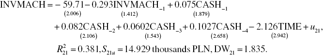

Figure 4.25 The actual quarterly investment outlays, the theoretical values of investments, and the residuals calculated on the basis of Equation 4.30.
Figure 4.26 displayed the actual monthly investments, the theoretical values, and the residuals calculated on the basis of Equation 4.31. Figure 4.27 analyzed the actual quarterly investment outlays for machinery and equipment, its theoretical values, and the residuals calculated on the basis of Equation 4.32. All Equations 4.30–4.32 are characterized by low accuracy in explaining the enterprise’s investment principles. A downward trend is a common feature of the overall investment or the investments in machinery and equipment. It indicates that the strategy of a dynamic development was abandoned in favor of the care for the company’s survival. The investments implemented after the 2000, essentially, were “forced.” Thus, a necessary replacement of old delivery vehicles by new ones followed, due to their excessive exploitation expenses and a risk of malfunction, since using the hitherto vehicles threatened regularity of the sales network servicing.

Figure 4.26 The actual monthly investments, the theoretical values, and the residuals calculated on the basis of Equation 4.31.

Figure 4.27 The actual quarterly investment outlays for machinery and equipment, its theoretical values and the residuals calculated on the basis of Equation 4.32.
4.11 Equations of wage effectiveness
Effectiveness of human-labor resources was examined in Chapter 4 using stochastic equations, which describe labor efficiency. Labor efficiency, analyzed earlier on, measured the ratio of the production volume to the resource meter of human-labor resources (the number of employees). Currently, the denominator in the formula used to calculate labor efficiency is going to be expressed by a variable of a streaming character, in the form of the enterprise’s payroll size. Thus, we will consider the following equations of wage effectiveness, where the efficiency meter is in the formula’s ratio
is going to successively contain each of the variables representing production.50
An empirical equation describing productive efficiency of the net payroll (ESAL), based on monthly time series, is as follows:

The set of explanatory variables in Equation 4.26 (outside the autoregressive dependencies) clearly differs from the set making up the equation describing a quarterly volatility mechanism of payroll’s productive efficiency. Autoregressions of the 2nd, the 11th, and the 12th order show a sequential reference of the variable ESAL’s value to its current level. On the other hand, autoregressions of the 4th, the 7th, and the 10th order indicate commutativity of the variable ESAL’s volatility during the indicated time intervals.
The monthly time series revealed an impact of the average monthly pay (with a delay of 5 and 6 months) and of the technical devices (with a delay of 2 and 7 months). As such, an impact of conventional factors of human-labor effectiveness occurs and it is characterized by a variety of time-delays.
Large time fluctuations of the variable ESAL cause the explanatory variables of Equation 4.34 to explain only 67.0% of its overall volatility. All stochastic characteristics of the considered equations are correct. Also, Figure 4.28 does not arouse a feeling that the empirical equation was wrongly fit to the actual data.

Figure 4.28 The actual monthly ESAL values, the theoretical values, and the residuals calculated on the basis of Equation 4.34.
The first empirical equation of the considered block of equations describes the variable SALPR, which expresses the relation of the ready-made production to the net payroll. An equation based on quarterly time series has the following form:

Figure 4.29 presented the actual quarterly EPL values, the theoretical values, and the residuals calculated on the basis of Equation 4.35. Economic efficiency of the net payroll is characterized by autoregressions of the second and the fourth order. This dependency, resultant from a delay by 2 quarters, signifies commutativity of the variable SALPR’s fluctuations every 2 periods, that is, an efficiency decline occurs after its increase and an increase in efficiency measured in this way is a consequence of this decline.

Figure 4.29 The actual quarterly EPL values, the theoretical values, and the residuals calculated on the basis of Equation 4.35.
Indicator of the noncurrent assets’ renewal is a statistically significant factor of the wage expenses’ efficiency, meaning both its current level as well as its size achieved in a previous quarter. Modernization of the assets53 fosters a simultaneous increase in the variable SALPR’s value, as evidenced by the parameter assessment by the variable FIXD, equal to −0.227. In contrast, improvement of the FIXD index in a previous quarter worsens the current wage efficiency, while deterioration of this characteristic fosters wage efficiency.
Equation 4.35 fairly accurately describes the mechanism of the quarterly net payroll’s efficiency, since explanatory variables explain around 83.1% of the SALPR’s volatility. Additionally, the theoretical values of the variable SALPR, calculated on the basis of Equation 4.35, differ from the empirical values of this variable, on average, by 77.5 cents (PL: grosz) of the ready-made production’s value per 1 PLN of net wages.
Next equation is going to describe a formation mechanism of the variable ESBRSL, which measures the relation of the sales income (SBRUT) to the net payroll (SAL). An empirical equation describing the variable ESBSL on a monthly basis has the following form54:

The structure of Equation 4.36 is considerably more complicated compared to all previous similar constructions. Besides autoregressive dependencies of the 2nd, the 6th, and the 12th order, there are the so-called classic impacts, including an impact of the average net wage with various delays as well as an impact of the technical devices also taking into account various delay periods.
Appearance of a significant impact of the variable SALDE on the sale effectiveness of the net wages – compared to the existing empirical results – is a novelty. Monthly dynamics of the variable SALDE in the years 1996–2002 are illustrated by Figure 4.30. The discussed variable turns out to be statistically significant, with the delays of 2, 4, 8, 9, and 10 months. An increase in the value of the SALDE index more often causes an increase in the sale effectiveness of the wages, rather than its decline. Three parameter assessments for the variable SALDE delayed by 2, 4, and 10 months, in fact, are positive. It can, therefore, be concluded that better financing of new techniques results in a higher, on average, wage effectiveness.

Figure 4.30 A single-base dynamics indexes of the variable SALDE in the years 1996–2002 (monthly, 1996, I = 100).
Empirical equation 4.36 highly accurately explains the mechanism of the variable ESBRSL’s volatility, since as much as 94.3% of its volatility results from the impact of a vast set of explanatory variables. Figure 4.31 confirms that opinion.

Figure 4.31 The actual monthly ESBSL values, the theoretical values, and the residuals calculated on the basis of Equation 4.36.
Next equations will describe a formation mechanism of the variable EFSAL, which measures the relation between the sales income and the net payroll. An empirical equation of the income efficiency of wages, based on quarterly data, has the following form:

Figure 4.32 illustrates the above equation.

Figure 4.32 The actual quarterly values of EFSAL, the theoretical values, and the residuals calculated on the basis of Equation 4.37.
A fourth-order positive autoregression in Equation 4.37 indicates repetitiveness of the variable EFSAL’s value every 4 quarters in a significant part of its volume. An increase in the sales income’s value by 1 thousand PLN per 1 thousand PLN of net payroll, prior to 4 quarters, entails a current increase of this variable’s value by 631 PLN of the sales per 1 thousand PLN of the net payroll.
Impact of the average net wages delayed by 1 and 4 quarters on the labor efficiency defined as such is significant. A negative sign of the assessment of the structural parameter by the variable APAY−1 draws attention. Additionally, a simultaneous impact of the variable FIXD on the variable EFSAL can be considered as a classic situation. Modernization of the noncurrent asset resources fosters sales efficiency of the pay and salary costs.
The positive impact of the variable RAN55 on the wage efficiency is interesting. It results from the fact that during the periods of increased sales of the assortments, the sales income increases significantly, at a less dynamic increase in the net payroll. The period of purchasing the stationery, related to the beginning of a school year, as well as purchasing of the calendars for the following year are characterized by a higher number of assortments, which appear on the issued invoices.56 The result is a higher sales income per 1 thousand PLN of the payroll being paid out.
Next equation describes labor effectiveness as a quotient of the cash inflows (CASH) and the net payroll (SAL), expressed by the variable ECS. An empirical equation expressing formation rules of the variable ECS on a monthly basis has the following form:

The last empirical equation of wage effectiveness contains up to 20 explanatory variables. Autoregressive dependencies (of seven variables) and impacts of the variable FIXD with various delay periods (seven variables) are dominant. Again, a significant role of technical devices in the formation of an economic wage effectiveness (TAL−7, TAL−10, and TAL−12) has revealed itself. The average net pay (APAY−5, APAY−12) is still important for effectiveness. Compared to previous empirical results, a negative linear trend, which occurred in the discussed meter of net wage effectiveness, is a new element. Confirmation of this trend can be seen in Figure 4.33.

Figure 4.33 The actual monthly EPLW values, the theoretical values, and the residuals calculated on the basis of Equation 4.38.
Compared to the other empirical equations that were constructed based on monthly time series, the volatility of ECS in Equation 4.28 was explained by the equation’s variables in 90.1%. The actual and the theoretical values of the variable ECS, in this case, are slightly different, which is shown in Figure 4.33.
Next two equations describe labor effectiveness as the ratio of the amounts of cash inflows and the net payroll, expressed using the variable ECS. An empirical equation based on quarterly data has the following form:

The nature of Equation 4.39, to some extent, is similar to Equation 4.37. We are dealing here with autoregressions of the second and fourth order as well as with a significant positive impact of the average net wage delayed by 4 quarters. The technical devices of machinery and equipment (TAM) delayed by 4 quarters turn out to be a brake for the variable ECS. This may result from a physical process of machinery aging, which results in its higher failure rate reflected through cash efficiency of the wage.
A significant impact of the variable FIXD on the variable ECS, both in the simultaneous and the delayed by 4 quarters values, does not require commenting. Figure 4.34 is an illustration of the mechanism described by Equation 4.39.

Figure 4.34 The actual quarterly EPLW values, the theoretical values, and the residuals calculated on the basis of Equation 4.39.
4.12 Equations of the efficiency of implementing the fixed assets
The last group of equations detached from the econometric model of a small-sized enterprise is going to characterize the size of the production effects generated by involving the tangible fixed assets in use. Two variables are going to be described:
- EFMACH – the ratio of the ready-made production’s value (PROD) and the initial value of active machinery and equipment57 (MACH),
- EFBFIX – as the ratio of the sales income to the initial value of the active fixed assets.58
All equations of effectiveness of the fixed assets are autoregressive-trended in nature.
The variable EFMACH is described by the following empirical equation obtained on the basis of monthly time series:

An important analogy can be seen in a monthly mechanism of the variable EFMACH’s volatility when compared to the equation for quarterly data. Description accuracy is slightly smaller than in case of quarterly time series. Only 59.9% of the volatility of the machinery and equipment’s monthly productivity is explained by autoregressions of the 4th, the 7th, and the 12th order as well as by a trend in the form of a third-degree polynomial. This observation is confirmed by Figure 4.37. In Equation 4.40, there is no reason to reject the hypothesis about the lack of a first-order autocorrelation of the random component ( Figure 4.35).59
Figure 4.35 The actual monthly EFMACH volumes, the theoretical values, and the residuals calculated on the basis of Equation 4.40.
Autoregression of the 12th order indicates a sequential reference of EFMACH values with accuracy up to 12 months. This means that an increase in the ready-made production by a 1000 PLN per 1 thousand PLN of the machinery and equipment’s value, prior to 12 months, results in a current increase in EFMACH’s volume by 354 PLN of the ready-made production per 1000 PLN of the initial value of this group of the tangible fixed assets in use. Impacts of EFMACH−4 and EFMACH−7 indicate a change in the explanatory variable’s sign every 4 and 7 months.
An analogical empirical equation constructed on the basis of monthly data has the following form:

Equation 4.41 relatively accurately describes the variable EFBFIX’s monthly volatility, since 78.2% of its volatility is explained by autoregressive relations of the 1st, the 4th, the 11th, and the 12th order as well as by a polynomial trend of the 3rd order. Equation’s residuals do not exhibit an autoregressive process of the first order.60 Figure 4.36 confirms a relatively high explanation precision of the EFBFIX’s mechanism. Sequential linkage of the productivity levels of the noncurrent assets occurs every 1, 11, and 12 months. A sign change, as a result of an autoregressive relation, occurs every 4 months. Clearly, it can be seen that the volatility of EFBFIX is oscillatory in character and, in the end, depends on the assortment structure of invoiced deliveries as well as on the demand that is changing seasonally.

Figure 4.36 The actual monthly EFBFIX volumes, the theoretical values, and the residuals calculated on the basis of Equation 4.41.
Next empirical equation based on quarterly data has the following from:

Equation 4.42 describes formation of the efficiency of the machinery and equipment’s use with moderate accuracy. Autoregressions of the second and the fourth orders as well as a trend in the form of a polynomial of the third order explain 79.5% of the total volatility of the variable EFBFIX. Equation’s residuals are a realization of the pure random component, since in the equation there is no first-order autocorrelation61 of the random component.
It is illustrated by Figure 4.37.

Figure 4.37 The actual quarterly values of EFMACH, the theoretical values, and the residuals calculated on the basis of Equation 4.42.
Equation 4.42 indicates that the fourth-order autoregression in the variable EFBFIX means that an increase in the ready-made production by 1 thousand PLN per 1 thousand of the initial value of machinery and equipment, prior to 4 quarters, entails an increase in the current level of EFBFIX by 273 PLN of production per 1000 PLN of the variable MACH. Autoregression of the second order indicates commutativity of the variable EFBFIX’s volatility every 2 quarters. An increase in this variable is followed by a decline in its value after 2 quarters, which in turn causes another increase – after two periods.
4.13 Practical applicability of a small-sized enterprise’s model
An econometric model of a small-seized enterprise mainly can be used for forecasts estimation of endogenous variables. It can also serve as an analysis tool allowing assessment of the effects of various possible decisions.62 For instance, company’s marketing strengths influence its production results. Those marketing strengths can be represented by various exogenous variables, characterizing the company’s marketing activity. Examples of such variables can be as follows: a variable representing advertisement expenses, a variables characterizing participation in fairs, and many others. This group of variables belongs to a category of decisional variables, called the steering variables. If the model contains statistically significant steering variables, then analysis can be performed using the model – of the effects of various values of particular decisional variables on the entire economic system. It will allow selection of most rational level variants of the steering variables, in terms of the decision maker’s needs (the manager’s needs).
Let us look at a hypothetical closed cycle of relations of type 4.3. An attempt to present a forecasting mechanism based on quarterly data will be made

From the empirical equation 4.30, it can be inferred that empirical simultaneous impact of the cash inflows on investment value does not exist. As a result, prediction from the sequence of relations 4.3 is going to have the nature of a chain sequence and is going to occur according to the following chain of relations:
As such, it is going to be necessary to estimate the forecast INVTp in the first instance, using a predictor based on the empirical equation 4.30, that is:

Quarterly forecasts of investment volumes, calculated using GRETL package, are presented in Table 4.1 and on Figure 4.38.
Table 4.1 Quarterly forecasts of investments for the year 2003 (in thousands PLN).
| Forecasted period | Forecast INVTp | Average prediction error | Forecast range (95% trust level) |
| 2003:1 | 3.910 | 12.4795 | −22.308 ÷ 30.129 |
| 2003:2 | −18.017 | 12.4795 | −44.236 ÷ 8.201 |
| 2003:3 | 12.881 | 12.4795 | −13.337 ÷ 39.100 |
| 2003:4 | −16.410 | 12.4795 | −42.628 ÷ 9.809 |

Figure 4.38 Quarterly forecasts of investments for the year 2003 (in thousands PLN).
Negative values of the forecasts of INVTp in the second and the fourth quarter of 2003 are rarely noticed. These values ought to be regarded as zero values. With the automatism contained within the predictor 4.44 illogical negative investment results appear. Thus it can be inferred that investments in the enterprise can occur in the first quarter at a level of close to 4 thousands PLN and in the third quarter – of a value of close to 13 thousands PLN.
It should be remembered that subjecting investments to a regular mechanism is difficult in a small-sized enterprise; for instance, purchases of machinery in connection with the so-called opportunity, where adequate cash resources must be gathered as a result of the variable CASH’s mechanism. Variable INV in a small company is an important decisional variable (steering variable), which stays in relation with the cash inflows. It is highlighted by the mechanism described in Equation 4.30, in which quarterly cash inflows delayed by 1 and 4 quarters are the investment stimulators.
Another variable forecasted for quarterly FIXAS data from the chain 4.43, described by Equation 4.27, is empirically explained by a first-order autoregression and by impact of the delayed variable CASH−4. In the empirical equation 4.27, the variable INV occurring in the hypothetical chain 4.43 was eliminated. Statistically insignificant delayed variables INV−1, INV−2, INV−3, and INV−4 were also deleted. As a result autonomous predictor, which allows estimation of forecasts FIXASTp, emerged:
Forecasts of the value of the fixed assets FIXASTp during subsequent quarters of 2003, estimated using the predictor 4.45, are presented in Table 4.2 and in Figure 4.39.
Table 4.2 The company’s quarterly forecasts of the values of the fixed assets, for the year 2003 (in thousands PLN).
| Forecasted period | Forecasts of FIXASTp | Average prediction errors | Forecast range (95% trust level) |
| 2003:1 | 541.036 | 13.7160 | 512.512–69.560 |
| 2003:2 | 538.288 | 18.6254 | 499.554–77.022 |
| 2003:3 | 540.582 | 21.9297 | 494.976–86.187 |
| 2003:4 | 547.262 | 24.3724 | 496.577–597.947 |

Figure 4.39 The company’s quarterly forecasts of the values of the fixed assets in use, for the year 2003 (in thousands PLN).
These forecasts indicate that in the subsequent quarters of 2003 oscillations around the value of about 540 thousands PLN can be expected. Most likely, this will result from small investment outlays. These forecasts are characterized by high precision. Relative prediction errors are at the level from ![]() to
to ![]() .
.
Having the forecasts INVTp and FIXASTp allows forecast estimation of the other variables from the chain 4.43, that is, PRODTp, SBRUTTp, and CASHTp. The predictors used for estimation of these forecasts will emerge from the empirical equations 4.17, 4.15, and 4.13. Attention should be paid to the fact that it is necessary to have a significant number of explanatory variables in the predictor PRODTp. Forecast estimation performed using the GRETL package requires much concentration and attention.