
4
Geotechnical Site Investigation and Soil Behaviour under Cyclic Loading
4.1 Introduction
As discussed in Chapter 2, foundation design requires not only ground profile but also information on wind, waves, and site‐specific geohazards, including natural hazards (e.g. seismic). However, this chapter is devoted to ground investigation, i.e. data and ground/soil parameters necessary for foundation‐related design. Site Investigations related to ground are necessary for the following:
- Foundation design for the turbine support structure and offshore substation structure. See Chapter 1 for a typical wind farm layout.
- Cable route. Chapter 1 shows the layout of a wind farm, and there are two types of cables (inter‐array and export cables) to transmit the electricity generated to the onshore grid. Investigations are necessary along the cable route for design purposes. The major considerations are: scour prediction, cable protection, and turbidity changes in the water. Turbidity changes in water will have implications in the fish population, thereby impacting the environment.
- Planning and analysis of installation of foundations, together with the seabed anchoring of installation vessels. For example, jack‐up vessels are often used to install the foundation, and a detailed ground profile is necessary for jack‐up vessel leg penetration analysis. Other examples are suction pressure required to install foundations or vibratory/impact energy for driving piles.
- Geo‐hazards at the wind farm site, which include slope stability (submarine slides) or presence of gassy soils. Seismic analysis would require prediction of liquefaction susceptibility of the ground and site‐response analysis.
Detailed coverage on all these aspects are beyond the aims and scope of the book. There are many books and specialised reports available on offshore site characterisation and ground investigations, and they will be referenced here for further reading. The aim of this chapter is to discuss soil parameters that are necessary for preliminary and detailed design calculations, including soil‐structure interaction (SSI) analysis. The testing methods through which these parameters are obtained are discussed and where possible further reading are suggested.
Arguably, ground‐related issues are one the greatest project risks due to the uncertainties in the predicted costs due to installation and the problems associated with it. For example, delays in installation will have a direct impact on capital expenditure (CAPEX) cost, project schedule, and therefore profitability. Often, construction methodologies can lead to health and safety issues and also to environmental damage, which could, in turn, lead to penalty as well as negative publicity of the developer. All the above can be avoided as far as practicable using knowledge of the site. The aim of the discussion is to highlight the importance of thorough site investigation.
4.2 Hazards that Needs Identification Through Site Investigation
Ground‐related hazards depend on the location of the wind farm. SUT (2014) classifies hazards into three types:
- Man‐made hazards. Examples include existing infrastructure such as oil and gas pipelines either on the seabed or buried, communication cables, shipwrecks, jack‐up footprints, unexploded ordnance (UXO), etc.
- Natural seabed hazards. These include, as the name suggests, rock outcrops, seabed topography, large diameter boulders, and unstable and steep slopes, etc.
- Subsurface geological hazards. Examples include rapidly changing stratigraphy, buried infilled channels, igneous intrusions near seabed, tectonic faults, gas hydrates zone, and presence of gassy soils, etc.
The readers are referred to SUT (2014) for a comprehensive list of hazards. Once the hazards are identified, it is necessary to assess the risk and impact of those to the projects.
4.2.1 Integrated Ground Models
Essentially, the integrated ground model is a way to manage and sort information in a meaningful way so that ground risks can be captured and communicated to various stakeholders of the projects. Examples of stakeholders include investors, due diligence personnel, insurers or underwriters, certifiers, asset owners, etc. SUT (2014) defines a ground model as a database of information that includes structural geology, geomorphology, sedimentology, stratigraphy, geohazards, and geotechnical properties of the site.
The development of ground model and managing geotechnical risk is an iterative process that involves collecting relevant data and then interpreting and presenting in a meaningful way. Ground models are constantly updated as more information is available. Obtaining offshore ground data (geological, geophysical, and geotechnical) is expensive, as it involves mobilising a vessel. Therefore, ground models are not usually finalized until after the business decision of wind farm development is made. Development of the ground model is a continuous process and may begin through the use of satellite images and desk study (i.e. geological information of the site).
4.2.2 Site Information Necessary for Foundation Design
A typical offshore wind farm consists of large number turbines widely spaced and therefore change in water depth and geology may be expected. Therefore, the investigation will cover a large amount of area together with the plausible route for cables. To carry out feasibility studies as well as create a detailed design, various information and data are necessary. Table 4.1 lists the essential ones.
Table 4.1 Site information and why it is needed.
| Type of data | Information required | Remarks on the use of data for design purpose |
| Metocean data: This involves meteorological and oceanographic condition at the wind farm location | The main information typically gathered are:
|
Wind speed, wave height and period, current speed, and water depths are needed for foundation load calculations. Current data are required for scour prediction and design of the cable route. Wave and wind (magnitude and frequency) data are necessary for fatigue life calculations. Wind and wave data are required to understand the nature of the load in terms of one‐way or two‐way. |
| Seismic and tsunami hazard | Location and nature of faults around the site which includes historical occurrences. For further details see Chapter 2. | This are needed for PHSA (probabilistic seismic hazard assessment) and DSHA (deterministic seismic hazard assessment). The output will be seismic hazard parameters for seismic load estimation. |
| Slope stability and seabed mobility | Slopes in the seabed around the area. Any history of subsidence, i.e. presence of any oil and gas reservoir under the seabed or gassy soils. |
Estimation of the ground subsidence (if any) around the foundation. Seabed mobility will determine the extent of unsupported length in the lifetime of the project and the scour protection measures needed to avoid such problem. |
| Site characterisation, which is a combination of geological, geophysical and geotechnical |
The strength and stiffness profile of the ground along the depth. For simplified calculations of monopile stiffness as shown in Chapters 5 and 6, two parameters are required: (a) Stiffness of the ground at one diameter depth; (b) Variation of the ground stiffness with depth. |
Strength of soil is required for ULS calculations, i.e. capacity of the foundations. Stiffness of the ground is required for prediction of foundation stiffness, which is necessary for natural frequency calculations and deformations. |
| Other considerations |
Marine growth studies, corrosion, and site‐specific considerations. For example, in European waters there are still plenty of UXOs. Environmental studies are likely needed. |
Long‐term prediction of capacity and load demand. |
4.2.3 Definition of Optimised Site Characterisation
The ground engineering requirement covers a large area and there are significant costs associated with mobilisation of an offshore site investigation vessel. Therefore, at the planning stage, it is necessary to develop understanding of the project's needs and requirements so that necessary data and soil samples for the project can be obtained from one mobilisation of a vessel. For the purpose of foundation design, the main requirement is the development of design ground profile and assigning engineering parameters to each of the soil strata. This is one of the most important and critical steps that demand expertise. Section 4.3 provides typical examples of design ground profile.
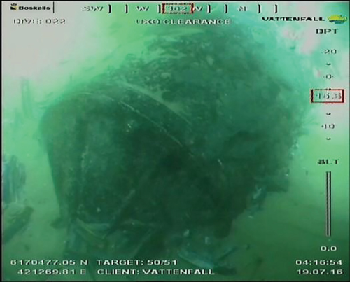
Figure 4.1 UXO in Horns Rev wind farm
(Source: [Photo Courtesy: Vattenfall]).
4.3 Examples of Offshore Ground Profiles
4.3.1 Offshore Ground Profile from North Sea
This section provides examples of typical ground profiles from a few offshore locations. Figure 4.2 and Table 4.2 shows a design ground profile from North Sea site following Bhattacharya et al. (2009). The location of the site is provided in Figure 4.3.
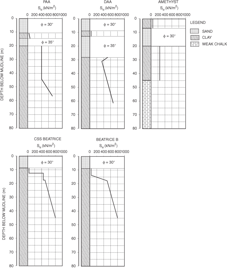
Figure 4.2 Example of offshore ground (Design profile) from North Sea. For location of these sites, see Figure 4.3.
Table 4.2 Soil profile at the sites.
| Location and time of the test | Relevant soil Layer (typical) |
| Beatrice field, PAA jacket site |
0.0–9.0 m sand (φ = ∼30°) 9.0–12.5 m soft to firm clay; (40–50 kPa) 12.5–17 m/29 m sand (φ = ∼35°) >17 m/29 m very hard clay (400–700 kPa) |
| Beatrice field, DAA jacket, |
0.0–8.5 m sand (φ = ∼30°) 8.5–12.5 m soft to firm clay (40–50 kPa) 12.5–29.0 m sand (φ = ∼35°) 12.5–15.0 m stiff to hard clay (40–500 kPa) >29 m very hard clay (400–700 kPa) |
| Amethyst field |
0.0–7.0 m stiff clay (40–150 kPa) 7.0–20.0 m medium dense sand (φ = ∼30°) 20.0–45.0 m stiff clay (∼250 kPa) >45.0 m very weak chalk |
| Beatrice field (North Sea), block 11/30, |
0.0–8.6 m medium to dense sand (φ = ∼30°) 8.6–12.6 m soft to firm clays (∼ 40 kPa) 12.6–17.6 m HARD CLAY (400–500 kPa) >17.6–45 m hard to very hard clay (500–800 kPa) |
| Beatrice field (North Sea), block 11/30, B jacket (adjacent to CSS) |
0.0–9.0 m loose very silty fine sand to dense fine sand (φ = ∼30°) 9.0–14.0 m soft sandy very silty clay (∼ 40 kPa) 14.0–18.0 m stiff to hard clay (40–500 kPa) >18.0 m hard to very hard clay(500–800 kPa) |
Other ground profiles from European wind farms are discussed in Chapter 5.
4.3.2 Ground Profiles from Chinese Development
There are four main sea areas in Chinese water where offshore wind development is in progress: (i) Bohai Sea (enclosed sea); (ii) Yellow Sea; (iii) East China Sea; (iv) South China Sea. Generally, the ground conditions in China seas are soft and layered, in contrast to North Europe.
For example, the Bohai Sea is a low‐lying land settled by North China Plain, where the soil consists of sediments brought from mountains and Yellow River and is soft, silty clay or clayey silt. Borehole is usually a widely used method for underground geology survey. There are many records of boreholes in Bohai Sea, and a typical profile (from top to bottom) is as follows:
- Soft clay silt (Layer 1). The depth of this layer varies but is typically 0–7.4 m in the western Bohai.
-
Mucky clay to silty clay (Layer 2). In this layer, the clay is changing from soft to stiff, with materials of mucky clay, silt, and loose sand. The depth of the clay layer varies (thickness 2.5–9.0 m in western Bohai), centre Bohai (thickness 4.0–10.0 m), Jinzhou (thickness 2.7–14.8 m) and Suizhong (thickness 0.8–5.8 m).
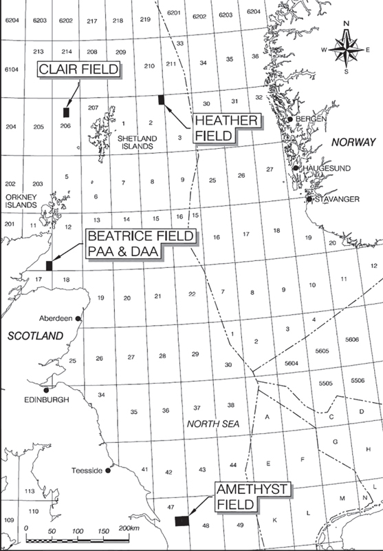
Figure 4.3 Location of the offshore sites. - Combination of silty clay, clay, and loose sand (Layer 3). Again, the thickness of this layer varies − 2.5–7.0 m in western Bohai.
- Fine sand and silt. In this layer, the main material is fine sand, combined with silty sand and clay. The stiffness is that of medium dense sand. The thickness in western Bohai is sea is 4.0–15.0 m, in centre Bohai is 4.0–13.0 m, in Jinzhou is 3.0–15.0 m, and in Suizhong is 0–14.2 m.
- Clay. In this layer, the clay is quite stiff and hard, combined with some silty clay. The thickness in western Bohai is 2.0–18.0 m, in centre Bohai is 3.0–15.0 m, in Jinzhou is 3.0–17.0 m, and in Suizhong is 0–15.0 m.
- Fine sand and silt
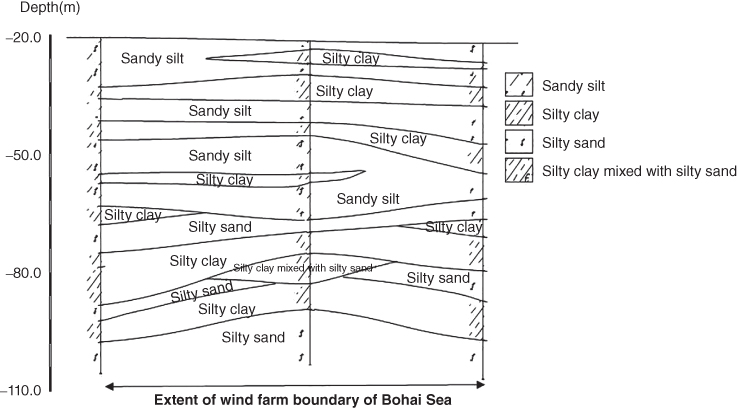
Figure 4.4 Ground profile in Bohai Sea wind farm.
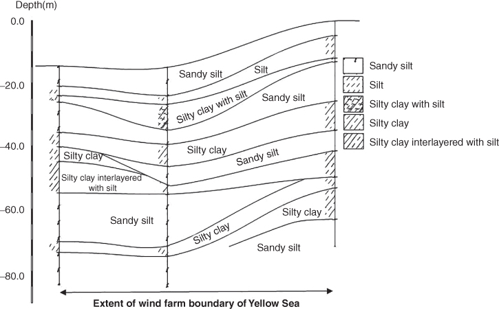
Figure 4.5 A section of a ground profile in Yellow Sea showing the extreme geology.
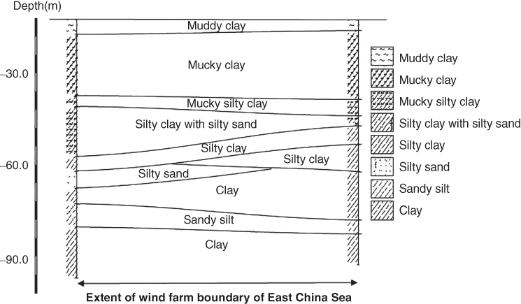
Figure 4.6 A section of the ground profile in East China Sea.
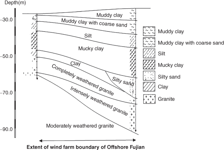
Figure 4.7 Ground profile in offshore Fujian Sea (Taiwan Strait).
In this layer, the main material is fine sand, combined with silty clay where the layer is thin. The stiffness is quite dense. The thickness in western Bohai is 5.0–11.0 m, in centre Bohai is 6.0–15.0 m, in Jinzhou is 7.0–15.0 m, and in Suizhong is 12.0–18.0 m (see Figure 4.4).
By contrast, Figure 4.5 shows ground profile for the Yellow Sea, and it is evident that the ground profile is variable, which calls for detailed site investigation to minimise risks during construction. Figures 4.6 and 4.7 show the ground profiles for other two Chinese seas.
Table 4.3 shows the ground profile in South China Sea. A general observation can be made. The ground profile in Chinese waters is variable, and it shows the importance of a comprehensive site investigation ( Table 4.3). Further details can be found in Bhattacharya et al. (2017).
Table 4.3 Ground profile in South China Sea.
| Position no. | Depth (m) | Soil |
| 1 | 0–4.2 | Silty clay |
| 4.2–19.4 | Laminated soil | |
| 19.4–40.0 | Silty clay | |
| 2 | 0–3.0 | Sandy soil |
| 3.0–7.4 | Silty clay | |
| 7.4–27.0 | Laminated soil | |
| 27.0–35.3 | Silty clay | |
| 3 | 0–1.9 | Silty clay |
| 1.9–2.6 | Silty sand | |
| 2.6–5.5 | Silty clay | |
| 5.5–9.0 | Sandy soil | |
| 9.0–15.0 | Laminated soil | |
| 15.0–39.8 | Silty clay | |
| 4 | 0–1.5 | Sandy soil |
| 1.5–4.9 | Silty clay | |
| 4.9–7.0 | Silty sand | |
| 7.0–13.7 | Laminated soil | |
| 13.7–25.4 | Silty clay | |
| 25.4–40.6 | Sandy soil |
4.4 Overview of Ground Investigation
The site investigation for offshore wind farms can be divided into three categories: geological, geophysical, and geotechnical. These are used to develop a comprehensive integrated ground model.
4.4.1 Geological Study
Chapter 1 showed that an offshore wind farm must cover a large area in order to maximise the energy yield. As shown, in some cases, the area is as large as 20 × 6.5 km. A study based on geological history of formation can be the basis of planning site investigation. Geological study is typically a desk study and is used to create the first ground model.
4.4.2 Geophysical Survey
This involves mobilising specialist vessels to map the seabed surface as well as subsea floor and the data generated can be used to update the ground model. A geophysical survey can be conducted alongside geotechnical site investigation. Table 4.4 shows the list of geophysical equipment for geophysical survey and design data/information obtained. Geophysical surveys are often carried out before the final business decision is taken.
Table 4.4 Types of geophysical survey.
| Geophysical equipment | Design data | Remarks |
| Multi‐Beam Echo Sounder (MBES) | Water depth and seabed topography of the whole wind farm and the cable route is obtained. | The bathymetry survey system and is generally hull‐mounted with sensors to compensate for vessel movement. Survey line spacing depends on the site |
| Side scan sonar (SSS) | Seabed features are recorded | Provides an acoustic image of the seabed |
| Sub‐bottom profiler | Ground profile and geology | Depending of the sub‐bottom resolution (e.g. pinger, sparker, boomer), they are required for shallow seabed for inter‐array or export cables or correlation of deeper layers in the geological model |
| Magnetometer/ Gradiometer | Unexploded ordnance (UXO) | These are used to map the change in magnetic field around a ferrous object |
DNV‐OS‐J101 suggests that line spacing of survey at the seabed location should be sufficient to detect all soil strata of significance for the design and installation of the wind turbine structure. It is also recommended that the survey needs to detect any buried channels with soft infill materials.
An example of an alignment chart used in a cable route investigation is given in Figure 4.8. The chart shows bathymetry, seabed features, sub‐bottom profile, magnetometer, route planning, and service chart.
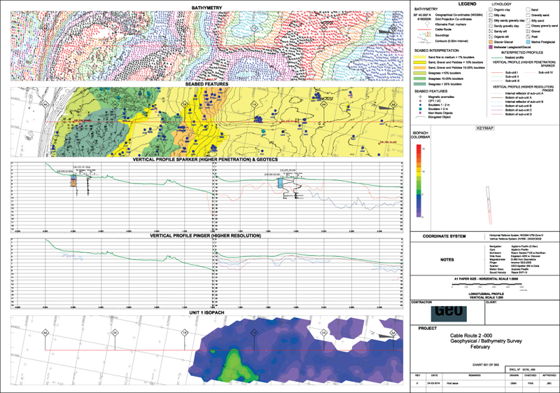
Figure 4.8 Alignment chart for cable route. [Photo Courtsey: GEO, Copenhagen].
4.4.3 Geotechnical Survey
The geotechnical site investigation required is governed by the foundation concept likely to be used and is, in turn, dependent on water depth, geology of the area, and the environmental conditions. In this process, a vessel is chosen depending on the requirements of the project for in‐situ testing and sample recovery from boreholes. Typically, in‐situ investigation involves pushing a cone (also known as cone penetration test, CPT) at different location to measure the soil resistance to penetration, see Figure 4.11 for an example bore log. Selection of vessel depends of various factors, and a summary of the important ones are given in Table 4.5.
Table 4.5 Vessel selection.
| Types of site | Vessels |
| Shallow water depth (typically less than 15–20 m) and good seabed conditions | Jack‐ups are suitable and standard onshore equipment can be used. |
| Water depth more than 20 m | Barges or ship with dynamic positioning system. |
| Site with high current | Anchored vessels with heave compensators |
Further details on the types of vessels can be found in Dean (2010), SUT (2014), and Rattley et al. (2017). Geotechnical investigation will provide the engineering parameters for the following analysis and design of: (i) foundations and its installation; (ii) inter‐array and export cables along a defined route; (iii) long‐term prediction in terms of serviceability limit state (SLS) and fatigue limit state (FLS). Some examples are: axial capacity of piles in tension and compression, p‐y curves for laterally loaded pile design, pile driveability characteristics, and bearing capacity of shallow foundations.
Typically, a geotechnical site investigation campaign involves the following:
- CPT at many locations to a depth depending on the types of foundations. A tentative guidance on the depth of penetration is given in the next section.
- High‐quality samples are obtained at selected locations through boreholes.
- In‐situ measurement of small strain stiffness may involve the use of a pressuremeter, dilatometer, or seismic cone.
- Laboratory testing (Table 4.6) provides a list of tests that are necessary. However, this is not an exhaustive list.
Table 4.6 Engineering parameters that are required for various calculations.
| Description and Index properties of the soil | Atterberg limit, maximum and minimum void ratio, water content of the sample | This is a fundamental property and many engineering correlations are based on these properties. These tests are often carried out in‐situ in the exploration vessel. |
| Strength properties of the soil | Friction angle (peak as well as critical state angle), undrained strength of soils. The following apparatus may be used: direct shear box, triaxial apparatus (e.g. CU/UU tests, consolidated / unconsolidated undrained) | These parameters are necessary for ULS calculations. The stress–strain graph is required for SLS and FLS calculations |
| Stiffness properties of the soil | In‐situ stiffness may be measured. For laboratory testing, the following apparatus may be used: resonant column, triaxial or cyclic triaxial with bender element, cyclic simple shear apparatus | Stiffness at small strain (G max) is one of the important parameters for natural frequency estimate |
| Permeability and consolidation parameters | Triaxial tests can be used or permeameters or CPT | Permeability information is required for assessing if the SSI interaction is drained or undrained. |
| Liquefaction potential | This is required for earthquake studies. Cyclic triaxial tests can be carried out to find the cycles to liquefaction and post‐liquefaction behaviour. | The analysis can predict the depth of liquefaction. A multi‐stage triaxial test (first cyclic load and then monotonic load) can also be carried out for post‐liquefaction behaviour. |
| Thermal conductivity | Thermal needle method may be used. Details of method can be found in Mitchell and Kao (1978), Farouki (1981, 1982) | This is required for cable insulation and protection design. |
| Chemical composition | To find the content of gassy soils and other chemicals that can cause corrosion to different buried components | Cable protection design |
| Damping properties | The following apparatus may be used: Resonant column and cyclic loading apparatus (cyclic triaxial and cyclic simple shear). | Damping measurement and are necessary for dynamic analysis of the whole system. |
4.5 Cone Penetration Test (CPT)
CPT initially developed in the 1950s in Holland, also known as the Dutch Cone Test, is one of the most used site investigation tools. The test consists of pushing an instrumented cone (together with a friction sleeve), with the tip facing down, into the ground at a controlled rate (typically 15–25 mm s−1). The standard cone has an apex angle of 60° and a cross‐sectional area of 10 cm2 corresponding to a diameter of 3.56 cm; see Figure 4.9. Electrical transducers measure the soil resistance on the cone tip as it penetrates into the soil. The frictional resistance along the sleeve is also measured. Another variation of CPT, known as CPTU, measures simultaneously tip resistance (q c), the sleeve friction (f s), and the pore pressure generated during penetration (u). In saturated soils, especially in fine‐grained soils, the development of excess pore water pressure reduces the value of tip resistance q c. Different proportions of sleeve friction f s and tip resistance q c for measured for different soils. Coarse‐grained soils will have high q c and low f s. On the other hand, fine‐grained soils will have high f s and low q c. Standard correlations and calibration charts exist for classifying soils; see Figure 4.10. Specialist knowledge is required for interpreting CPT data, and the readers are referred to Lunne et al. (1997) and Robertson et al. (1986).
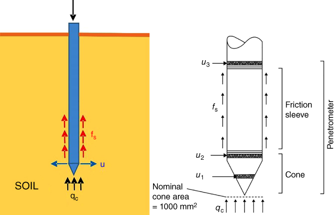
Figure 4.9 CPT test.
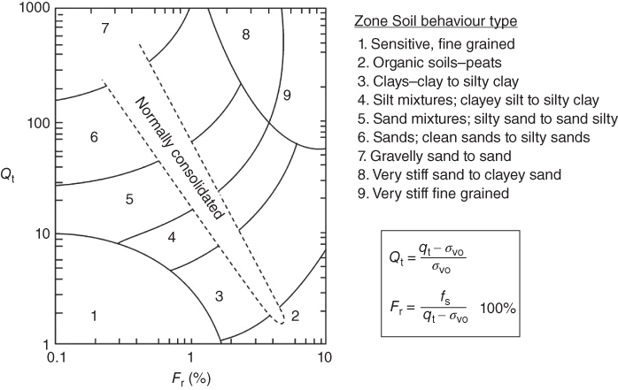
Figure 4.10 Soil classifications based on CPT.
Table 4.7 provides a preliminary guide for the relation between cone resistance (q c) and the angle of internal friction ϕ (o) in fine sand. It should be noted that this guide is applicable to unaged, uncemented sands up to about 10–15 m depth.
Table 4.7 Correlations of cone resistance and angle of internal friction.
| Cone resistance, q c (MPa) | Compaction of fine sand | Relative density, D r (%) | Angle of internal friction, ϕ (o) |
| <2 | Very loose | <15 | 20–25 |
| 2–5 | Loose | 15–35 | 25–30 |
| 5–15 | Medium dense | 35–65 | 30–35 |
| 15–30 | Dense | 65–85 | 35–40 |
| >30 | Very dense | 85–100 | >40 |
The results from the CPT test can also be used to estimate soil strength and stiffness.
To estimate the soil strength and assess the undrained shear strength of a soil (S u), the net resistance from the CPT q net (corrected cone resistance minus the vertical stress) is divided by a cone factor (N kt).
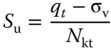
where typical N kt factors for the North Sea are 15–20.
In terms of stiffness, empirical equations suggested by different researchers may be used to estimate shear velocity and shear modulus. A few examples are given below:
The cone resistance can be used to determine the shear modulus of different sands using either of the following relationships Rix and Stokoe, (1991), Mayne and Rix, (1993):
where e is the soil void ratio:
The cone resistance can also be used to determine the shear velocity ( V s ) as given.
4.6 Minimum Site Investigation for Foundation Design
Many codes of practice and best practice guides, such as the DNV, American Petroleum Institute (API) and SUT (2014), provide guidance for the minimum site investigation requirements and this section summarises them. For wind turbine structures in a wind farm, a tentative minimum soil investigation program may contain four aspects:
- One CPT test per turbine location for a grounded system based on monopile. For suction buckets, and other foundations such as floating/anchored foundations, one CPT for each suction bucket or anchored location will be needed.
- Soil boring to sufficient depth in each corner of the area covered by the wind farm for recovery of soil samples for laboratory testing. This will provide a basis for variability of the ground.
- An additional soil boring in the middle of the area will provide additional information about possible non‐homogeneities over the area.
- In cases where soil conditions are highly varying within small spatial areas and foundations, more than one soil boring or more than one CPT per wind turbine position may be needed.
In‐situ testing such as CPT and soil borings with sampling should be carried out to sufficient depths. The following are recommended:
- For slender and flexible piles in jacket type foundations, a continuous CPT from seabed to the anticipated depth of the pile plus three times pile diameters is recommended.
- For monopile with larger diameters, a continuous CPT from seabed to the anticipated depth of the pile plus 0.5 times the pile diameter is recommended.
- For gravity‐based system, a sample borehole or deep continuous CPT borehole at the centre of the proposed structure. The number and depth of borings will depend on the soil variability in the vicinity of the site. This is necessary for settlement predictions.
- For jack‐up installation vessels, the CPTs performed for the wind turbine generator (WTG) foundation are often used. Otherwise, depth equal to at least one and a half spudcan diameter are recommended.
4.7 Laboratory Testing
Once the offshore samples are recovered, laboratory tests must be carried out to obtain as much information as possible. It will be shown in Chapter 5 that soil−structure interaction plays an important role in the long‐term performance of these structures and, as a result, advanced soil tests are necessary. The types of tests depend on the types of foundations and the nature of loading. It must be mentioned that the cost of laboratory tests is negligible when compared with the cost required to obtain them.
4.7.1 Standard/Routine Laboratory Testing
The most commonly used element testing methods are direct shear and ring shear tests, simple shear tests, triaxial tests, and consolidation tests. The readers are referred to textbooks on element testing for details and methodology. Some examples are Dean (2010), Mitchell and Soga (2005), Head (2006), and Randolph and Gourvenec (2011). Table 4.8 provides a summary on the soil parameters that can be obtained from such tests.
Table 4.8 Routine element tests.
| Name of the test | Description of the test | Requirement in design |
| Direct shear test |
This apparatus is used to determine shear strength parameters. It consists of horizontally split, open metal box where one part of the box can move relative to the other. Soil is poured in the box at a particular density and one part of the box is moved relative to the other. The soil is designed to fail in a thin zone along the interface of the two part box. This apparatus is commonly known as shear box. |
Drained tests are generally conducted in a Shear Box. Angle of friction ( ϕ ), Angle of dilation Undrained strength (cohesion). Shear Box cannot prevent drainage i.e. pore pressure cannot be measured. Undrained shear strength can be estimated approximately by shearing the soil very fast, i.e. running the test very quickly) and the sample fails at the specific plane and not necessarily at the weakest plane. |
| Triaxial tests | Triaxial Test: A cylindrical soil sample is tested where confining pressure can be applied together with different drainage condition i.e. drained/undrained. Deformation of the soil along with volume change/ pore water pressure change can be measured. The main advantage is variety of stress and strain paths that a soil experiences in the field can be simulated. |
We can obtain: Stress‐strain characteristics of a soil, shear strength, and volume change together with pore water pressure Permeability of soil samples can also be measured. The following parameters may be obtained: Angle of friction ( ϕ ), cohesion/undrained strength (Su) Shear modulus ( G ) from the slope of the stress strain curve. |
| Oedometer test | This involves applying compression to a disk of soil vertically to obtain the time‐dependent characteristics. | Compressibility of the soil |
| Ring shear test | In this test an annular soil sample is twisted to induce a circular shear plane. | Residual friction angles for clay |
4.7.2 Advanced Soil Testing for Offshore Wind Turbine Applications
As discussed in Chapter 2, loads on the foundation are cyclic as well as dynamic. It is therefore necessary to understand the behaviour of soils under such loading conditions. From practical view of view, three types of apparatus readily available and widely used in engineering practice: cyclic triaxial with bender element, cyclic simple shear (CSS), and resonant column apparatus.
4.7.2.1 Cyclic Triaxial Test
The triaxial test is the most widely used and versatile shear strength test. As the name suggests, the soil specimen is subjected to compressive stresses in three directions by fluid pressure. To fail the soil sample, additional vertical stresses are applied on the top of the sample, axially (either monotonically or cyclically) by a loading ram. Different types of tests can be carried out: drained, undrained, consolidated undrained, and multistage. The basic features of the triaxial test apparatus are presented in Figure 4.12. Figure 4.13 shows a cyclic triaxial set at SAGE (Surrey Advanced Geotechnical Engineering) laboratory. The readers are referred to textbooks for further details of triaxial test procedures. This apparatus is widely used in earthquake engineering practice to study the problem of cyclic liquefaction of saturated granular materials. The response of soils can be represented by plotting stress path graph (p′ − q) where p′ and q are the mean effective stress and deviator stress, respectively, and the definition are given below:
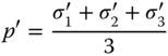
where, ![]() and
and ![]() are the maximum and minimum principal effective stress, respectively. In triaxial tests, it is assumed that the intermediate and the minimum principal stress are the same (i.e.
are the maximum and minimum principal effective stress, respectively. In triaxial tests, it is assumed that the intermediate and the minimum principal stress are the same (i.e. ![]() ).
).
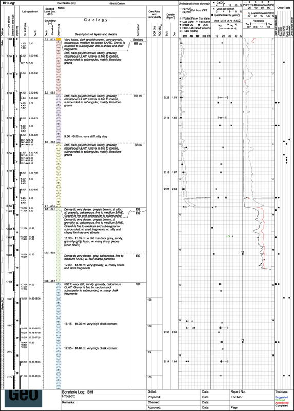
Figure 4.11 Typical example of a bore log and engineering parameters.
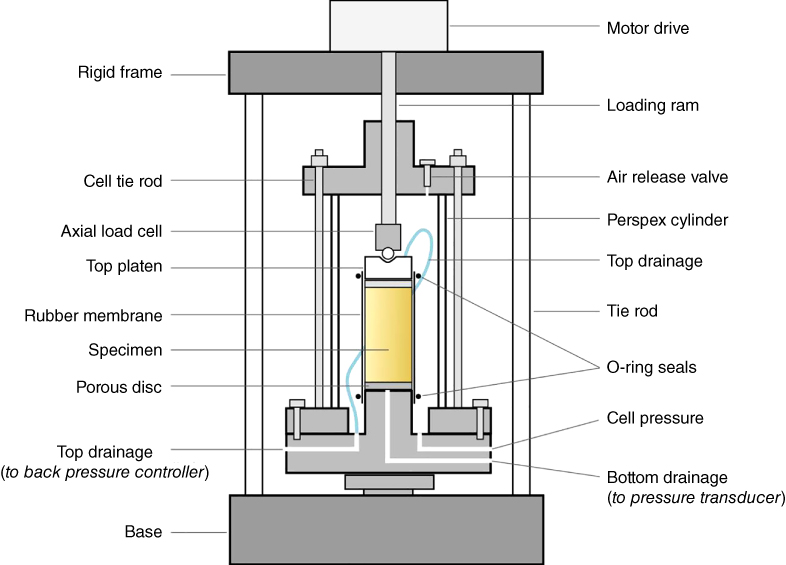
Figure 4.12 Schematic outline of a triaxial apparatus.
Both compression and extension cycles in the effective triaxial plane (q−p′) are usually performed. An example of a cyclic triaxial apparatus, under undrained conditions to simulate earthquake loading, is presented in Figure 4.14. The number of cycles necessary in undrained conditions for the material to reach a state of liquefaction is evaluated and the effective stress path is recorded. During the tests, both pore pressure within the sample and axial strain can be recorded (Figures 4.13 and 4.14).
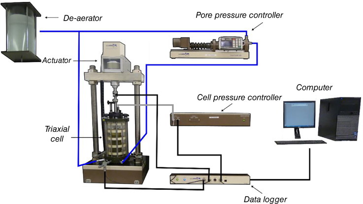
Figure 4.13 Schematic of the testing system from SAGE laboratory.
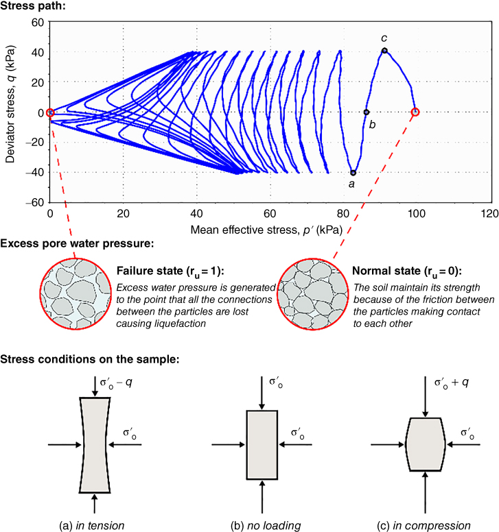
Figure 4.14 Typical result of a cyclic triaxial test, under undrained conditions.
Depending on the perceived imposed loading on the soil, loading stages can be generated or recreated. For example, Figure 4.15 illustrates the schematic diagram of the testing scheme adapted for the multistage soil element test to simulate an extreme case of soil liquefaction. In these tests, undrained stress‐controlled sinusoidal cyclic loading with a certain frequency and amplitude was initially applied in order to liquefy the soil sample. Once the specimen liquefied, cyclic loading was stopped and strain‐controlled monotonic load was then applied under undrained condition. This will provide the stress−strain curve of the liquefied sand. Figure 4.16 shows a result from the multistage test on Assam sand (India) to study liquefaction. Readers are referred to Rouholamin et al. (2017) and Dammala et al. (2017) for examples of multistage tests.
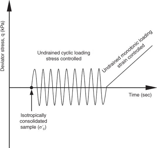
Figure 4.15 Testing scheme adopted for the multi‐stage element test to study extreme loading condition due to an earthquake.
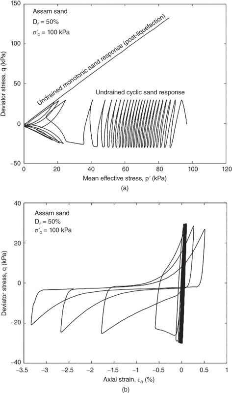
Figure 4.16 Multi‐stage test using cyclic triaxial on Assam sand (a) stress path; and (b) deviator stress versus axial strain during cyclic phase.
Bender element can be used to obtain the shear wave velocity of the sample through wave propagation technique. The cyclic triaxial text can be applied in two ways to issues related to offshore wind turbines:
- Cyclic triaxial apparatus, together with the bender element, can be used to study the effect of an extreme storm on long‐term performance. Cyclic loading may be applied to a soil sample corresponding to a storm to recreate the stress history. At the end of the loading, monotonic load may be applied to find the residual soil stiffness and strength.
- Based on the literature, the behaviour of standard soils such as pure clay or pure sand can be predicted with some degree of confidence. It is, however, difficult to predict the behaviour of intermediate soils, i.e. sandy‐silt or silty‐sand, or clayey‐silt, as the main question is whether the sample will behave like clay‐like material or sand‐like material. In other words, the behaviour of soils with varying amount of fines content is difficult to predict, and in such cases cyclic triaxial tests are useful. This will have a big impact on the prediction of long‐term behaviour, as it is the accumulation of pore water pressure in the soil that will dictate the behaviour due to the effects of millions of cycles of loading.
4.7.2.2 Cyclic Simple Shear Apparatus
Figure 4.17 shows a CSS apparatus together with the schematics of a sample shearing pattern taken from SAGE laboratory. The apparatus is capable of applying cyclic loads (both in vertical and horizontal direction) using two electro‐mechanical dynamic actuators. The vertical and horizontal displacements can be measured using encoders within the servo motors. Different wave forms can also be applied: sinusoidal, square, triangular, saw tooth, haversine. The apparatus is also capable of applying user‐defined waveforms. In the current context of offshore wind turbines, user‐defined functions can be used to simulate random wind and wave loading. This apparatus has been used in Nikitas et al. (2016) to study the long‐term performance of offshore wind turbine foundations.
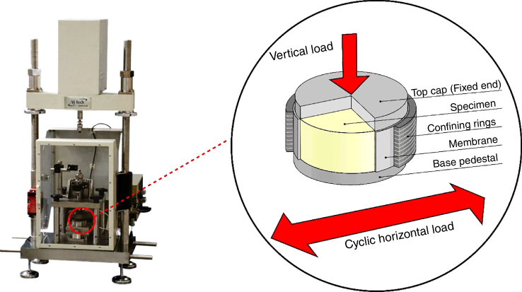
Figure 4.17 Experimental setup for cyclic simple shear test.
In the study, external LVDTs (linearly varying differential transformer) were also used to record displacements and to verify the effectiveness of feedback control. Loads up to ±5kN can be applied in two directions with horizontal travel up to 25 mm and vertical travel of 15 mm. These are sufficient to study the effects of large strain levels applied to the soil. This therefore allows the study of effects of cyclic shear stress under drained and undrained conditions. The loads can be applied at frequencies of up to 5 Hz. This apparatus was used to investigate the cyclic behaviour of a silica sand (typical of North Sea) by maintaining the constant vertical consolidation stress while cycling the shear strain in horizontal direction. Typical results are presented in Figures 4.18 and 4.19.
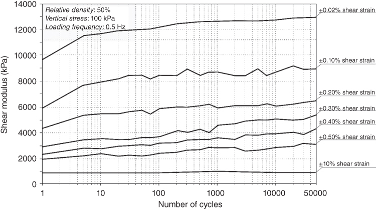
Figure 4.18 Results of red hill sand obtained from CSS apparatus.
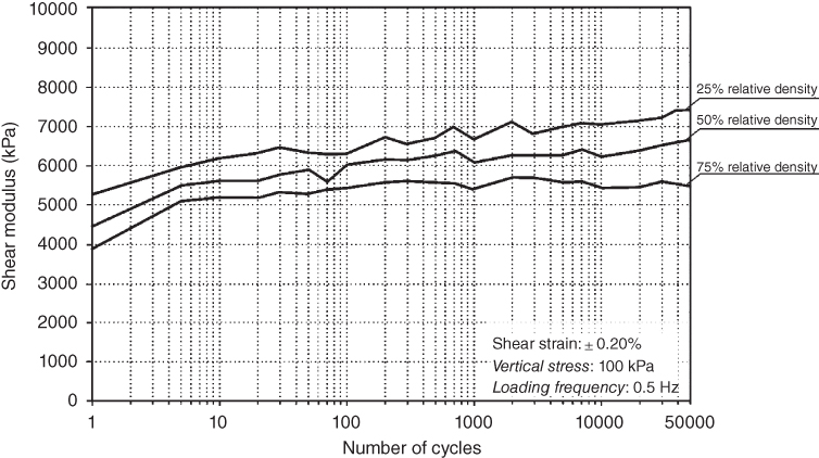
Figure 4.19 Results from CSS apparatus.
Carefully designed and performed tests can be useful in predicting the long‐term performance. Readers are referred to Chapter 5 for further details on the soil−structure interaction. The strain levels applied to the soil under different loading conditions from the turbine can be found in Section 5.5.
4.7.2.3 Resonant Column Tests
This apparatus can be used to map the change of stiffness for a wide range of strain levels. The basic principle involved in this test is the theory of wave propagation in prismatic rods where a cylindrical soil specimen is harmonically excited until it reaches the state of resonance (i.e. peak response). Figure 4.20 shows schematic diagram of a soil sample and the apparatus. Resonant column tests can be carried out to determine shear modulus and damping ratio of soil for a wide range of strain level.
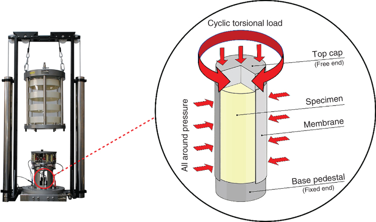
Figure 4.20 Schematic of resonant column testing layout, resonant column apparatus used at the SAGE Laboratory, University of Surrey.
This technique was first developed in the 1930s at the University of Tokyo by Ishimoto and lida (1936) and Ishimoto and lida (1937). The resonant column only saw wider use in the 1960s with the works of authors such as Hall and Richart (1963), Hardin and Richart (1963), and Drnevich et al. (1967). In the past few decades, a number of subsequent improvements and advancements have been made in resonant column testing to broaden the range of applicability. These have included the application of anisotropic stresses to the soil element (Hardin and Music 1965; Hardin and Black 1966), adaptations to the apparatus to hollow the testing of elements (Drnevich 1967), and modifications to tests specimens at large (Anderson and Stokoe 1978; Stokoe and Lodde 1978) and at high strains (Alarcon et al. 1986; Isenhower et al. 1987; Ampadu and Tatsuoka 1993).
Figure 4.20 shows a particular type of resonant column apparatus and it uses 50 mm diameter by a 100 mm long soil sample utilising a fixed‐free configuration. This arrangement is the most widely utilised resonant column arrangement in research as the mathematical derivations required are fairly simple. In such an arrangement a cylindrical soil element is excited in torsion by a dynamic drive system connected to the top cap. A simplified schematic can be seen in Figure 4.21. Through the resonant column tests, the damping ratio (D) of the soil can be measured from the free vibration decay curve (logarithmic decrement) using the accelerometer. Figures 4.22 and 4.23 show typical results from the resonant column test.
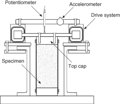
Figure 4.21 Simplified cross section schematic of one type of resonant column apparatus.
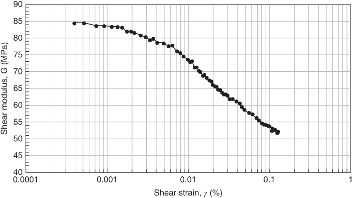
Figure 4.22 Shear strain‐shear modulus graph measured by the resonant column test on Redhill‐110 sand.
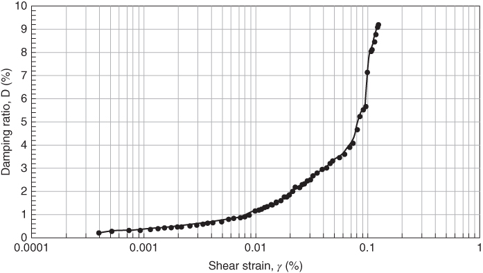
Figure 4.23 Shear strain‐damping ratio graph measured by the resonant column test on Redhill‐110 sand.
4.7.2.4 Test on Intermediate Soils
Figures 4.24 and 4.25 show the results from resonant column tests on four types of soils with varying fines content carried out at Yamaguchi University (Japan). The graphs show as expected the variation of stiffness and damping with strain level. Figure 4.25 shows the plot of accumulated pore water pressure with strain level. It is interesting to note that for strain level corresponding to G eq/G max of 0.6–0.85, pore pressure starts to build and that is the onset of progressive collapse.
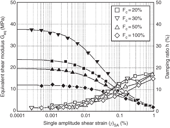
Figure 4.24 Stiffness and damping properties of soil with different strain levels.
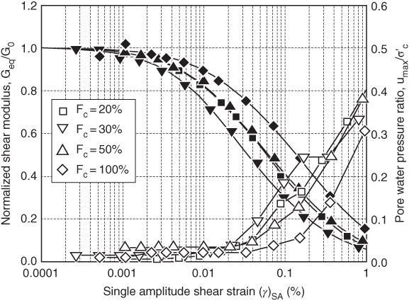
Figure 4.25 Pore water pressure build‐up with strain level.
4.8 Behaviour of Soils under Cyclic Loads and Advanced Soil Testing
Behaviour of soils under cyclic and dynamic loading is still an active area of research. Soil dynamics problems can be classified based on magnitude of strain levels, frequency of loading, and number of cycles as shown in Figure 4.26. Figure 4.27 shows the different classes of soil dynamics problem and full treatment of the problem will need an entire textbook.
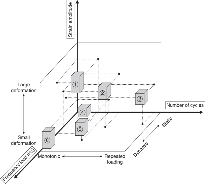
Figure 4.26 Classification of soil dynamics problem based on three parameters: frequency, number of cycles, and strain level.
4.8.1 Classification of Soil Dynamics Problems
The main aim of this section is to provide a summary of the issues related to offshore wind turbine problems. Explanation of the numbers is provided in Figure 4.26:
- Earthquake loading characterised by large strain, low number of cycles, and low frequency (0.5 to 10Hz)
- Loading on offshore structures
- Traffic loading
- Represents the strain in the soil due to variation of ground water table
- Pile driving, Soil compaction
- Impulsive load (Blast) characterised by high frequency, very low number of cycles and small deformation
4.8.2 Important Characteristics of Soil Behaviour
All soils under moderate cyclic loads yield progressively, try to compact, generate positive pore water pressure, and soften. Collapsible soils such as loose sands can liquefy in the absence of drainage. The frequency of cyclic loading condition is therefore important, since the pore pressure generated by one full load cycle may only partially dissipate before the next load cycle.
For clays, the strength and stiffness degrades. The amount of stiffness degradation is a function of strain level and the number of cycles of loading. Extensive laboratory and field studies have clarified many aspects of the behaviour of clays under such loading; see, e.g. Vucetic and Dobry (1991). Stiffness degradation has been correlated with the plasticity index (PI) of the soil. For a particular cyclic strain in the soil, more plastic clays exhibit less degradation. Figure 4.28 shows a graph based on 16 sets of published experimental data from strain controlled tests on clays having different PIs and OCRs. In the graph, a PI of zero indicates sand and a PI of 200 represents highly plastic Mexico City clays, which show little nonlinearity up to 0.1% cyclic shear strain. G max is the secant shear modulus at small strain. Figure 4.29 shows the effect of degradation on G/G max for different numbers of cycles (N = 1, 10, 100, and 1000) for normally consolidated clays (OCR of 1).
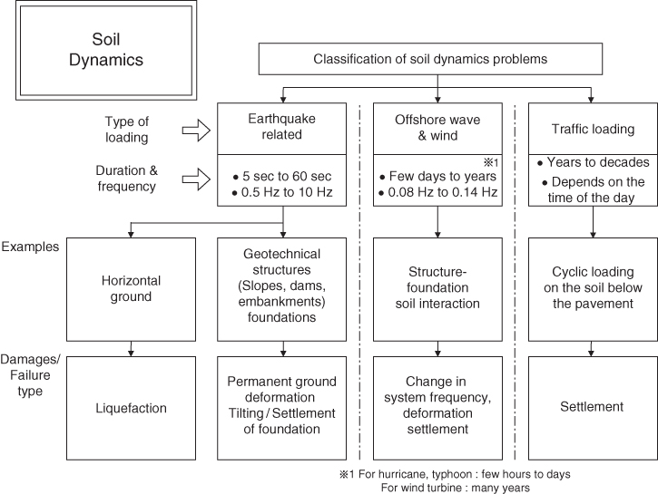
Figure 4.27 Classification of soil dynamics problems.
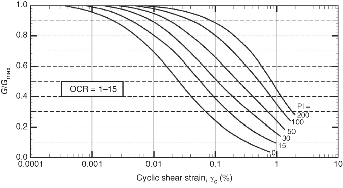
Figure 4.28 Relations between G/G max versus cyclic shear strain for NC and OC clays. [Source: Vucetic and Dobry (1991)].
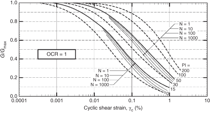
Figure 4.29 Effect of cyclic stiffness degradation on G/G max versus cyclic shear strain for soils having different PI and loaded to different number of cycles. [Source: Vucetic and Dobry (1991)].
When analysing a soil system, three important features of soil behaviour must be considered:
- Soil is a nonlinear material, in which the stiffness progressively decreases with increasing shear stress, until at a sufficiently high shear stress level it deforms plastically.
- Soil is an inelastic material. Therefore, when subject to cyclic loading, it exhibits hysteretic damping (energy loss), which increases with increasing shear strain.
- The soil properties, including strength, stiffness, and pore water pressure, may be affected by repeated cycles of load. This is particularly relevant to saturated sands and silts that may suffer a build‐up in pore water pressure with continued load application possibly resulting in liquefaction.
Five main properties (bulk density, stiffness, material damping, strength, and degradation due to cyclic loading) determine the response of a soil‐structure system under dynamic load. The bulk density affects the inertia of the soil under dynamic loading. The stiffness, which is largely defined by the shear modulus, determines the natural frequency of the system and the response. Damping is a measure of energy dissipation: the higher the damping, the greater the energy loss and therefore, the smaller the response.
4.9 Typical Soil Properties for Preliminary Design
When carrying out dynamic analyses, particularly in the early stages of projects, all the soil information will not be available. Table 4.9 provides a range of standard parameters, which can be used for preliminary design if no other data are available. Readers are referred to Appendix A of Bhattacharya et al. (2019) for full details of many more correlation.
Table 4.9 Typical soil properties that may be used for preliminary design.
| Soil Type | Description | φ′ (°) | su (kPa) | G max (MPa) |
| Gravel | Dense | 40 | – | 230 |
| Sand |
Loose Medium Dense |
30 32.5 35 |
– – – |
10 20 55 |
| Silt | – | 25 | – | 10 |
| Clay |
Soft Firm Stiff |
– – – |
25 50 100 |
2 30 60 |
| Rock |
Mudstone Sandstone Granite |
– – – |
– – – |
2150 3100 15 700 |
4.9.1 Stiffness of Soil from Laboratory Tests
Initial stiffness of the soil (i.e. soil stiffness at small strain) is an important parameter for design. Laboratory tests suggest that the maximum shear modulus (G max) can be expressed by Eq.
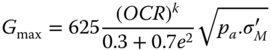
In another form, Eq. (4.7) can be expressed as G max = 625 F(e) (OCR) k pa 0.5 (σ M ′)0.5 where F(e) is a function of void ratio and k is an OCR exponent, which varies with PI, as shown in Table 4.10.
Table 4.10 Variation of OCR exponent (Hardin and Drnevich 1972).
| PI | 0 | 20 | 40 | 60 | 80 | 100 |
| k | 0 | 0.18 | 0.3 | 0.41 | 0.48 | 0.5 |
Hardin (1978) proposed that F(e) = 1/(0.3 + 0.7e 2), while Jamiolkowski et al. (1991) suggested that F(e) = 1/e 1.3. Please note that G max, p a and σ M ' must all be expressed in the same units. p a is atmospheric pressure.
Ishibashi and Zhang (1993) suggest the relationship between shear modulus G and its maximum value G max for fine grained soil:
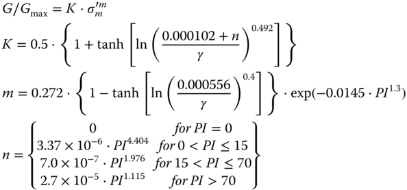
where, σ′ m is the mean principal effective stress, γ is the shear strain, and PI is the PI of soil.
For cohesive soils, the relationship between G 0/S U, PI, and OCR as summarised by Weiler (1988) can be used Table 4.11.
Table 4.11 Gmax/sU values.
| OCR | |||
| PI (%) | 1 | 2 | 5 |
| 15–20 | 1100 | 900 | 600 |
| 20–25 | 700 | 600 | 500 |
| 34–45 | 450 | 380 | 300 |
In addition to the theories proposed above, Seed and Idriss (1970) derived a simplified equation to describe the low strain stiffness for any granular material. As all formulations are strongly influenced by confining pressure and void ratio, only these factors were considered leading to the following derivation;
where:
| p′ | Mean local effective stress | [kN m−2] |
| K 2 | Soil modulus coefficient | [−] |
The coefficient K 2 itself has been experimentally derived from a number of different sands. It was found that under low strain conditions (γ < 10–3%) the soil modulus coefficient only depends on the void ratio (Seed et al. 1984). Typical values for K 2 are detailed in Table 4.12 taken from guidelines. The readers are also referred to updated correlations.
Table 4.12 Soil modulus coefficient for a number of typical sand densities (Det Norske Veritas 2002).
| Soil type | K 2 |
| Loose sand | 8 |
| Dense sand | 12 |
| Very dense sand | 16 |
| Very dense sand and gravel | 30–40 |
4.9.2 Practical Guidance for Cyclic Design for Clayey Soil
The salient features are:
- Soil stratification and type of soil at the top layers. For a deep foundation, it is the top soil that deforms most.
- What is the scour depth?
- For soils, it is required to predict under what condition, pore water pressure will start to accumulate?
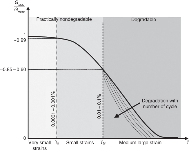
Figure 4.30 Secant shear modulus reduction curve for fully saturated clay subjected to cyclic undrained loading.
Figure 4.30 shows the variation of normalised secant stiffness with strain for fully saturated cohesive soil adapted from Vucetic (1994). It is accepted that there exists a strain level, the threshold linear shear strain, γ tl , for which there is no stiffness degradation and the behaviour of the soil is practically linear elastic, so that there is no permanent microstructural changes of the fabric of the soil with cyclic loading. As the strain level is increased beyond γ tl , the soil behaves nonlinearly and as a result the secant shear modulus of soil will reduce. The value of γ tl can be estimated from the secant shear modulus reduction curve (schematically shown in Figure 4.30) assuming that linear threshold shear strain corresponding to a ratio G sec/G max of 0.99. There exists another value of threshold shear strain, known as volumetric threshold shear strain level (Vucetic 1994), denoted by γ tv , beyond which permanent microstructural changes of the fabric do occur. In other words, beyond γ tv the soil is degradable possibly due to pore pressure build‐up. In the triaxial stress space, this state corresponds to the boundary between the ‘recoverable’ and the ‘plastic zone’ (Jardine 1992). γ tv can be assessed from the secant shear modulus reduction curve. However, two value of G sec/G max ratios (namely, 0.85 and 0.60) are often used, depending on the application. The value of 0.85 represents a degradation of secant shear modulus beyond which permanent deformation is expected. On the other hand, 0.6 is defined on the basis of the accumulation of excess pore pressures. These two values can represent upper and lower bound values of γ tv for the problem in hand. The upper bound value will give the highest diameter that may be required. On the other hand, the lower bound will give the minimum diameter necessary. It is interesting to note the graphs presented in Figures 4.24 and 4.25 showing the pore water pressure build‐up. While Figure 4.30 shows the schematic representation of threshold strains, Figure 4.31 plots typical experimental data obtained from cyclic triaxial tests carried out on 10 samples of Turkish clay having a PI ranging from 9 to 40 following Okur and Ansal (2007).
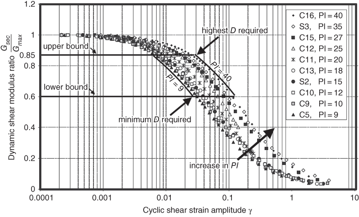
Figure 4.31 Experimental secant shear modulus reduction curve for samples of Turkish clay with different PI.
Figure 4.31 shows an upper and lower bound for γ tv which corresponds to G sec/G max ratio of 0.85 and 0.60, respectively. The experimental results clearly show that samples with higher PI tend to have a more linear cyclic stress−strain response at small strains and to degrade less at larger strain than soils with lower PI. Therefore, clays with higher PI are characterised by higher values of volumetric threshold shear strain. For example, considering the lower bound, γ tv increases from 0.025 to 0.15 when PI increases from 9 to 40.
Figure 4.32 collates the volumetric threshold shear strain value ( γ tv ) for 18 types of clays having PI ranging from 9 to 100. The experimental data were collected from research published by Kim & Novak (1981), Kokusho et al. (1982), Vucetic & Dobry (1988), Georgiannou et al. (1991), Lanzo et al. (1997), Stokoe et al. (1999), Massarsch (2004), Okur & Ansal (2007), Yamada et al. (2008). In the same figure, two linear correlations for evaluating γ tv are also suggested for the investigated range of PI (9 < PI < 100). The experimental data used for deriving the plot in Figure 4.32 are given in the Table 4.13.
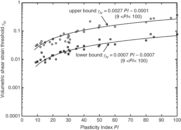
Figure 4.32 Volumetric shear strain threshold values for different PI.
Table 4.13 Data pertaining to graphs in Figure 4.31.
| Soil name | PI | OCR | Test apparatus | Reference |
| Windsor silty clay | 30 | 2.7 | Resonant column | Kim and Novak 1981 |
| Wallaceburg silty clay | 25 | 5.1 | Resonant column | Kim and Novak 1981 |
| Hamilton clayey silt | 12 | 5.8 | Resonant column | Kim and Novak 1981 |
| Sarnia silty clay | 14 | 1.8 | Resonant column | Kim and Novak 1981 |
| Alluvianal clay at Teganuma | 44, 57, 58, 83, 96 | NC | Cyclic triaxial | Kokusho 1982 |
| laboratory‐made clays | 15, 30, 50, 100 | NC | Not specified | Vucetic and Dobry 1988 |
| Vallericca clay | 31 | OC | Resonant column | Georgiannou et al. 1991 |
| Pietrafitta clay | 30 | OC | Resonant column | Georgiannou et al. 1991 |
| Todi clay | 28 | OC | Resonant column | Georgiannou et al. 1991 |
| laboratory‐made clay | 22 | 3 | Direct simple shear | Lanzo et al. 1997 |
| Fat clay | 36 | Not specified | Not specified | Stokoe et al. 1999 |
| Not specified | 10, 20, 40, 60, 80 | Not specified | Not specified | Massarsch 2004 |
| Turkish clay | 9, 10, 12, 15, 18, 20, 25, 27, 35, 40 | NC | Cyclic triaxial | Okur and Ansal 2007 |
| Ariake clay | 44 | NC | Hollow cylinder | Yamada et al. 2008a |
| Onada clay | 50 | NC | Hollow cylinder | Yamada et al. 2008a |
4.9.3 Application to Offshore Wind Turbine Foundations
The strain level in the soil next to the monopile i.e. the strain in the mobilised shear zone can be compared to the volumetric threshold strain, γ tv which is a fundamental property of a soil and can be obtained from soil testing. Section 5.5 in Chapter 5 presents a method to compute the soil strain and if the strain in the mobilised zone exceeds this threshold strain, degradation may be excepted. This concept is quite similar to the mobilisable strength design (MSD) concept pioneered by Osman and Bolton (2005) where the average strain in a mechanism (deformed zone or sheared zone) is linked with an element test in a soil. The above concept has been experimentally shown to be valid by Lombardi et al. (2013).
Choosing diameter of monopile for design: It will be shown in Chapter 5 that higher the diameter of the monopile, the lower is the average strain in the surrounding soil. Therefore, choosing a larger diameter pile will lower will be the degradation. The designer needs to make sure that if the strain level in the soil exceeds the γ tv for the clayey soils, adequate allowance for stiffness reduction needs to be taken into account.
4.10 Case Study: Extreme Wind and Wave Loading Condition in Chinese Waters
A typhoon can lead to failure or even collapse of wind turbines, especially in the region of East and South China Sea. Typhoons can have a negative effect on wind turbine systems ranging from fracture of blades, damage to braking system, yielding of tower, and even excessive rotation foundation. However, the direct effect of typhoon is loss of power supply and emergency shutdown, which may damage the weakest part (e.g. blade and nacelle). It is therefore necessary to understand the wind condition in the Chinese waters. This section provides a brief summary:
- Bohai Sea: The total area of the Bohai Sea in China is approximately 77 284 km2 and is classified in four parts: west, middle, Jinzhou, and Suizhong. Bohai Sea is the only inner sea region of China and is a shallow sea with average water depth of about 18 m. In the winter months, due to the flow of cold air from Siberia, the average wind speed is about 6–7 m s−1. On the other hand, in summer months, due to warm air flow from the Western Pacific Ocean, average wind speed is 4–5 m s−1. In August, the wind speed is quite low. In this sea, wind farms are located in Jinzhou and predominant wind directions for high wind speed are southeast and southwest with mean annual wind speed of 7.21 m s−1 (100 m height over sea level). Typhoons and cyclones are not normal in the Bohai Sea and the wind condition is stable throughout the year. Bohai Sea has a cold climate, and in the winter period the onshore near coastline is almost frozen for three to four months.
- Yellow Sea: The total area of Yellow Sea 380 000 km2 and comprises Shandong, Jiangsu, and Korean Peninsula. There are many offshore wind farms built along the coastline in Yellow Sea from north to south. In the winter, the wind is stable but in summer it varies in both magnitude and direction. Typhoons are very frequent in summer throughout Shanghai area, which is located in the south of Yellow Sea. The annual average wind speed in the north Yellow Sea is 6.80–6.88 m s−1 but in the south, the value is much larger and the average value is 7.45–7.55 m s−1.
- East China Sea: The total area of East China Sea is 770 000 km2 and comprises the continent coastline of Japan and Taiwan. There are many offshore wind farm projects located in Hangzhou Bay. The annual mean wind speed tested at 100 m in height over sea level is generally around 9.6–9.8 m s−1 at the exit of Hangzhou Bay. However, in terms of frequent typhoon phenomena in summer from May to September each year, wind speed remains unstable, and the value is quite large, even over 14 m s−1. Cyclone effect is very important and governs the design.
- Taiwan Strait: The Taiwan Strait is one part of East China Sea, connected with the South China Sea in the south of China. It is common to see the strong wind (e.g. typhoon) in summer and damage the cities and structures along coastline. Usually, typhoons in the summer will come from southeast and the wind speed is quite high, even much bigger in height. The annual mean wind speed in Taiwan Strait is about 11.5–13 m s−1. It will be over 20 m s−1 or more when a typhoon is coming. Each year, typhoons are the main natural disaster, which brings large damage to the economy and structure in Taiwan, Fujian, and Zhejiang Province, located on two sides of Taiwan Strait, respectively.
- South China Sea: The total area of South China Sea is about 3 500 000 km2. It is surrounded by the continent of South China mostly, northeast to Taiwan Strait, southwest to Singapore Strait. Most of the projects are newly built or under construction in recent years. It is also common to see strong wind (e.g. typhoon) and to bring rainwater in the summer each year. The annual mean wind speed in the South China Sea is 9–11 m s−1. When a typhoon comes, the wind speed is over 17 m s−1 usually (at 100 m in height). Table 4.14 summarises the wind conditions in the Chinese waters.
Table 4.14 Wind conditions summary in China Seas (unit: m/s).
| Sea name | Wind speed range (m s−1) | Mean wind speed (m s−1) |
| Bohai Sea | 6.4–8.2 | 7.45 |
| Yellow Sea (north) | 6.8–7.5 | 6.86 |
| Yellow Sea (south) | 7.0–8.2 | 7.48 |
| East China Sea | 7–11 | 9.68 |
| Taiwan Strait | 11.5–13 | 12.04 |
| South China Sea | 8.8–9.8 | 9.18 |
4.10.1 Typhoon‐Related Damage in the Zhejiang Province
Zhejiang Province, located on the west of East China Sea, experienced typhoon 23 times since 1997 (start time of wind farm project), causing hundreds of millions of dollars of economic loss. It is of interest to discuss the effects of 10 August 2006 Typhoon Saomai, which had 68 m s−1 wind speed that devastated many wind farms. This is the most powerful typhoon to hit China in a half century. It killed 104 people and left at least 190 missing. Furthermore, it blacked out cities and smashed more than 50 000 houses in the southeast part of the country. Figure 4.33 shows the Hedingshan wind farm in Zhejiang Province before the cyclone along with the aerial photograph of the typhoon. The typhoon destroyed 28 wind turbine structures and blades, including five tower collapses (600 kW turbine), with a total a loss of about 70 million RMB (Figures 4.34–4.36).
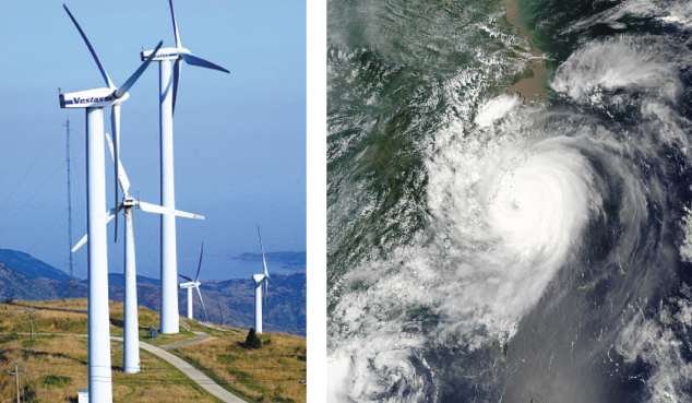
Figure 4.33 Hedingshan wind farm (before typhoon Saomai) and aerial view of the typhoon. [Photo Courtsey Prof Lizhong Wang].
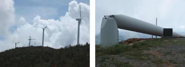
Figure 4.34 Damages to blades and tower due to typhoon Saomai. [Photo Courtsey Prof Lizhong Wang].
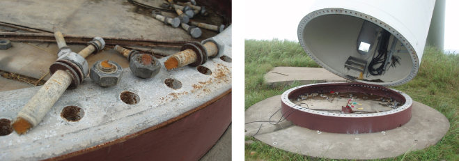
Figure 4.35 Damages to the connections.
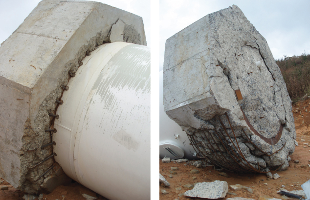
Figure 4.36 Damages to the foundations.
Table 4.15 Wave height and period in the Chinese waters.
| China Sea | Region | Wave height (m) | Wave period (s) |
| Bohai Sea | Bohai Strait | 1.2 | 4.8 |
| Others | <1 | <4.5 | |
| Yellow Sea | North | 1.2 | 5 |
| Centre | 1.4 | 5 | |
| South | 1.6 | 6 | |
| East China Sea | Shanghai coastline | 1.6 | 6 |
| Zhejiang coastline | 1.8 | 7 | |
| Taiwan Strait | 2.4 | 9 | |
| South China Sea | Luzon Strait | 2.8 | 10 |
| Indo‐China Peninsula | 2.6 | 8 | |
| Others | <2 | 6 |
4.10.2 Wave Conditions
Bohai Sea, Yellow Sea, East China Sea, and South China Sea are connected with each other, shaped as a bow from north to south along the China coastline. A tropical and subtropical monsoon climate also influences the China Sea waves. Thus, in Chinese offshore wind farm projects, sea wave is a main factor that influences the design. The wave height distribution in the South China Sea is variable owing to its large area of sea region. High wave height occurs northeast of South China Sea and southeast of the Indo‐China Peninsula, where waves are about 2.4–2.6 m in height. The maximum significant wave height is larger than 2.8 m west of the Luzon Strait. Comparatively, the significant wave height in the north is less than 2 m. Wave period ranges from 6 to 10 seconds, with similar distribution of wave height. Table 4.15 shows the distribution of wave height and period for the Chinese waters.
Chapter Summary and Learning Points
- Obtaining reliable engineering parameters for calculation is one of the most important tasks. Geological, geophysical, and geotechnical studies are necessary for a wind farm design. These studies can be integrated to form a ground model.
- Soil structure interactions for offshore wind turbines are complex. It will be shown in Chapter 5 that one of the workable solutions is to estimate the strain in the soil in the mobilised/deformed zone. This chapter describes the behaviour of soils over a wide range of strains.
- Element test of soils that can be carried out to understand the behaviour over a wide range of strain are described.