
5
Soil–Structure Interaction (SSI)
SSI for offshore wind turbine (OWT) supporting structures is essentially the interaction of the foundation/foundations with the supporting soil due to the complex set of loading. The readers are referred to Chapter 2 for discussion on loading. This chapter reviews the different aspects of SSI for foundations that are being used or proposed. Due to cyclic and dynamic nature of the loading that acts on the wind turbine structure, the dominant SSI will depend to a large extent on the global modes of vibration of the overall structure. This chapter discusses the various SSI and the available calculation methods.
5.1 Soil–Structure Interaction (SSI) for Offshore Wind Turbines
SSI will be affected in three main ways:
- Load‐transfer mechanism. The load transfers rom the superstructure to the ground through the foundation, and this is the soil–structure interaction whereby stresses are generated in the soil. Monopiles will load the soil very differently than jackets. For a monopile, the main interaction is lateral pile–soil interaction (LPSI) due to the overturning moment and the lateral load. On the other hand, for a jacket, the main interaction is the axial load transfer. Therefore, the SSI depends on the choice of foundation and essentially how the soil surrounding the pile is loaded. The readers are referred to Section 2.5 in Chapter 2 for further discussion on this topic. This mainly guides the ultimate limit state (ULS) criteria for foundation design.
- Modes of vibration. The modes of vibrations are dependent on the types of foundations, i.e. whether the foundation is a single shallow foundation or a summation of few shallow foundations or one deep foundation (monopile) or a combination of few deep foundations. Essentially, if the foundation is very stiff vertically – we expect sway bending modes, i.e. flexible modes of the tower. On the other hand, wind turbine generators (WTG) supported on shallow foundation will exhibit rocking modes as the fundamental modes. This will be low frequency and it is expected that there will be two closely spaced modes coinciding with the principle axes. Two closely spaced modes can create additional design issues: such as beating phenomenon, which can have an impact in FLS (fatigue limit state). Further discussions can be found in Section 3.2 in Chapter 3.
- Long‐term performance. Understanding SSI is important when predicting the long‐term performance of these structures. Based on the discussion in Chapters 2 and 3, SSI can be cyclic as well as dynamic and will affect the following three main long‐term design issues:
- Determine whether the foundation will tilt progressively under the combined action of millions of cycles of loads arising from the wind, wave and 1P (rotor frequency) and 2P/3P (blade passing frequency). Figure 2.21 shows a simplified estimation of the midline bending moment acting on a monopile type foundation, and it is clear that the cyclic load is asymmetric, which depends on the site condition, i.e. relative wind and wave component. It must be mentioned that if the foundation tilts more than the allowable, it may be considered failed based on SLS criteria and may also lose the warranty from the turbine manufacturer.
- It is well known from the literature and discussed in Chapter 4 that repeated cyclic or dynamic loads on a soil causes change in the properties, which, in turn, can alter the stiffness of foundation. A wind turbine structure derives its stiffness from the support stiffness (i.e. the foundation), and any change in natural frequency may lead to the shift from the design/target value and as a result the system may get closer to the forcing frequencies. This issue is particularly problematic for soft‐stiff design (i.e. the natural or resonant frequency of the whole system is placed between upper bound of 1P and the lower bound of 3P) as any increase or decrease in natural frequency will impinge on the forcing frequencies and may lead to unplanned resonance. This may lead to loss of years of service, which is to be avoided.
- Predict the long‐term behaviour of the turbine, taking into consideration wind and wave misalignment aspects. Wind and wave loads may act in different directions. The blowing wind creates the ocean waves, and ideally they should act collinearly. However, due to operational requirements (i.e. to obtain steady power), the rotor often needs to feather away from the predominant direction (yaw action), which creates wind–wave misalignment.
5.1.1 Discussion on Wind–Wave Misalignment and the Importance of Load Directionality
Following Chapter 3, the most important design drivers for foundation design are the ultimate, fatigue, and serviceability limit state requirements. The assumption of aligned wind and waves is acceptable for ULS design. However, when the long‐term performance is assessed, the directionality of wind and wave loading must be incorporated. This can be carried out probabilistically to assess the long‐term performance of OWT foundations, as shown by Arany (2017). The environmental state is represented by a Bayesian network of interdependent variables representing wind and wave parameters, wind direction, and wind–wave misalignment. The number of environmental states occurring in the lifetime of the turbine is generated through simple Monte Carlo methods, and a fast‐frequency domain approach is used to assess the damage for each environmental state. The complete lifetime simulation is repeated many times to establish the probability distribution of lifetime damage in different directions around the pile. It is demonstrated that the lifetime damage, taking into account load directionality, is significantly reduced compared to aligned wind and wave assumption.
This important aspect is demonstrated in Figure 5.1 through the use of fixed and moving coordinates. The notations of ξ and η directions are introduced for the along‐wind (fore–aft) and cross‐wind (side‐to‐side) directions, respectively. We further introduce another coordinate system fixed in space: north–south direction Y (with positive Y values pointing north), and the west–east direction X (with positive values towards the east). When discussing loads on the foundation, it is important to note that the ξ and η directions are not fixed in space, that is, the two coordinate systems (ξ,η) and (X,Y) have the same origin, but they do not coincide at all times. This is because the (ξ,η) coordinate system rotates with the nacelle yaw angle φ with the positive ξ axis being approximately normal to the rotor plane (neglecting the nacelle tilt angle) and points in the direction of the mean wind speed (neglecting nacelle yaw misalignment). This is important because when fatigue loads on the foundation have to be analysed, then the directions the designer should be concerned about are loads in the (X,Y) system, recognising that the foundation obviously does not rotate with the nacelle. It is also important to emphasise here that because of the above effect, all load directions in the (X,Y) coordinate system (that is, e.g. all sections around the circumference of the monopile) are subjected to load cycles due to both along‐wind and cross‐wind load processes throughout the lifetime of the turbine.
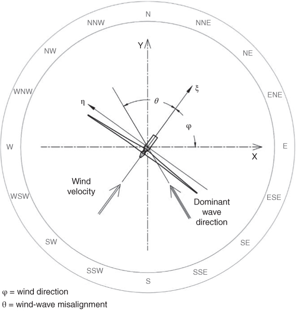
Figure 5.1 Spatially fixed (X,Y) and yaw angle‐following (ξ,η) coordinate systems.
If the most severe loads (incorporating the dynamics of the structure) can be demonstrated to act in the along‐wind direction and with collinear wind, waves, and currents, then it is a conservative to use this load scenario for ULS purposes. Not only the wind–wave misalignment but also the general direction of the load can be neglected for a circularly symmetric foundation (e.g. monopiles, caissons, or round gravity‐based structures), or a single‐most severe load direction can be chosen for a substructure without circular symmetry (jackets, tripods, floating structures, etc.). However, when assessing the number of load cycles throughout the lifetime, then assuming that all load cycles occur in the same direction produces overly conservative estimations for the total fatigue damage suffered by the structure or indeed the total number of load cycles causing accumulated tilt or deflection.
It is therefore essential to understand the mechanisms that may cause the changes in dynamic characteristics of the structure and if it can be predicted through analysis. An effective and economic way to study the behaviour (i.e. understanding the physics behind the real problem) is by conducting carefully and thoughtfully designed scaled model tests in laboratory conditions simulating (as far as realistically possible) the application of millions of cyclic lateral loading by preserving the similitude relations. The readers are referred to Bhattacharya et al. (2018), where scaled model tests for analysis and design of OWT foundations are discussed.
Considerable amount of research has been carried out to understand various aspects of cyclic and dynamic soil–structure interaction (DSSI); see, e.g. Leblanc et al. (2009), Lombardi et al. (2013), Bhattacharya et al. (2013a,b), and Bhattacharya (2014a,b). The studies showed that to assess the SSI, it is necessary to understand not only the loading on offshore wind turbines but also the modes of vibration of the overall system.
Years of offshore engineering practice have provided clarity regarding load transfer to the foundation. The methods to estimate the capacity of foundations have been developed and are available in codes of practices. By capacity, we mean the ultimate load‐carrying capacity of the foundation. Examples of commonly used foundations are given in this chapter, together with references for further reading.
Modes of vibration will dictate the interaction of the foundations with the supporting soil. Furthermore, if the foundation–soil interaction is understood, the long‐term behaviour of the foundation can be predicted through a combination of high‐quality cyclic element testing of soil and numerical procedure to incorporate them in different interactions.
5.2 Field Observations of SSI and Lessons from Small‐Scale Laboratory Tests
Limited monitoring of offshore wind turbines indicates that the dynamic characteristics of these structures may change over time and have the potential to compromise the integrity of the structure due to fatigue and resonance phenomena. A few examples are given here.
5.2.1 Change in Natural Frequency of the Whole System
Scaled model tests carried out by Bhattacharya et al. (2013a,b), Yu et al. (2014), Guo et al. (2015), and Cox et al. (2014) indicate that the natural frequency of a wind turbine system may change owing to dynamic soil–structure interaction. Change in the natural frequency of the Hornsea Met Mast structure supported on a twisted‐jacket foundation is also reported by Lowe (2012). Three months after the installation, the natural frequency dropped from its initial value of 1.28–1.32 to 1.13–1.15 Hz, shown schematically in Figure 5.2. On the other hand, Figure 5.3 shows the results from Lely wind farm following Kuhn (2000). In this figure, the design value of frequency is 0.4 Hz and the measured value after 6 years is 0.63 Hz.
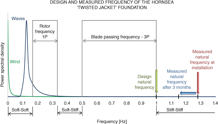
Figure 5.2 Change in natural frequency in a twisted‐jacket supporting a met mast.
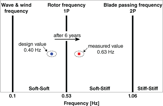
Figure 5.3 Frequency within a gap of 6 years from Lely wind farm reported in Kuhn (2000).
5.2.2 Modes of Vibration with Two Closely Spaced Natural Frequencies
As discussed in Chapter 3, as was observed in scaled model tests, there can be multiple resonance peaks for certain types of structure. This is indicative of closely spaced natural frequencies corresponding to different modes of vibration. This was observed and noted in Brent B Condeep platform, see Figure 5.4 which was selected for an extended instrumentation program sponsored by several oil companies operating in the North Sea. Accelerations were recorded and results plotted in frequency domain following Hansteen (1980). The two first modes of vibration are 1.78 seconds (0.56 Hz) and 1.72 seconds (0.58 Hz), representing bending modes in the two horizontal directions. The third mode of 1.19 s (0.84 Hz) corresponds to torsional mode of vibration.
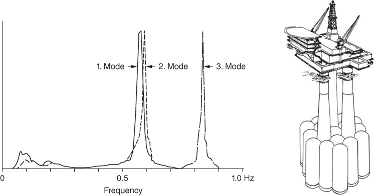
Figure 5.4 Observed multiple peaks for Brent B Condeep platform following Hansteen (1980) and image from of Condeep platform from Oide and Andersen (1984).
It is of interest to discuss some aspects of the Condeep (Concrete deep water structure) structure, shown in Figure 5.4. The foundation consists of 19 cells having an overall diameter of 100 m resting on 45 m of stiff‐to‐hard overconsolidated clay with some layers of dense sand. The structure is designed for 100 years wave height of 30 m.
5.2.3 Variation of Natural Frequency with Wind Speed
A schematic sketch of the measured difference between the design and actual natural frequency of the Siemens SWT‐3.6‐107 type 3.6 MW turbines at the Walney 1 site is shown in Figure 5.4. There are two salient features: (i) The difference of 6% between prediction and observed is reasonable, given the complexity of the structure and the uncertainty in the calculation methods mainly the ground stiffness measurements; (ii) scatter increases on natural frequency at higher wind speed until about 14 m s−1. As wind speed increases, the moment at the foundation increases, which will increase the strains in the soil. As discussed in Chapter 4 , with increasing strain level, stiffness of soil decreases and damping increases. Another interesting point to note is that as the wind speed increases beyond 14 m s−1, the controlling action will kick in (either pitch control or yaw control) and the load on the foundation will not increase. This may explain the reduction in the scatter (Figure 5.5).
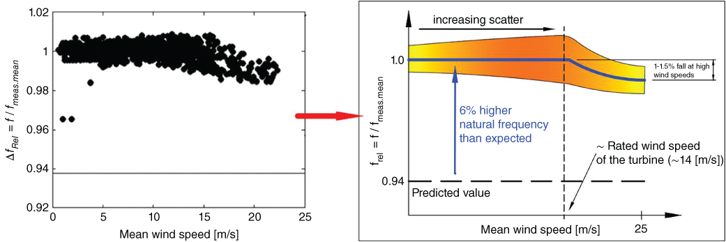
Figure 5.5 Measured and predicted natural frequency at Walney site. The figure in the left‐hand side (LHS) is provided by Kallahave et al. (2012) and the interpretation is provided in the schematic sketch in right‐hand side (RHS).
5.2.4 Observed Resonance
Resonance has been reported in a wind turbine site in the German North Sea under operational conditions. Figure 5.6 shows the frequency domain plot based on Hu et al. (2014). The explanation of resonance is due to the proximity of the natural frequency to the 1P and 3P.
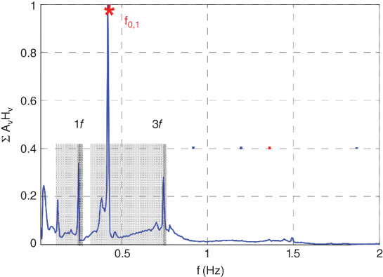
Figure 5.6 Observed resonance in German North Sea following Hu et al. (2014).
5.3 Ultimate Limit State (ULS) Calculation Methods
Based on the design considerations presented in Chapter 3 , together with the discussion presented in Section 5.1, this section lists the different ULS calculations that are necessary. The ULS is of critical importance to the foundation design and is usually the first step. These are available in many textbooks and therefore are not repeated here. Some notable textbooks and monographs are Dean (2010), Randolph and Gourvenec (2011), Encyclopaedia of Maritime and Offshore Engineering (2018), and Salgado (2006).
5.3.1 ULS Calculations for Shallow Foundations for Fixed Structures
Section 1.5.1 of Chapter 1 provides different types of shallow foundations for WTG structures. They are often a good alternative to deep foundations in good ground conditions, and their stability depends on their weight. Often, jackets are temporarily supported on shallow foundations (essentially a steel plate known as mudmats) before their main fountains are driven. The shapes of shallow foundations can be rectangular, square, or circular in plan. They can be even multicellular, and for mudmats the shape can be irregular. To improve load‐bearing capacity, skirts are often attached to the foundations. The load acting on such foundations are: vertical load (V), moment (M), and horizontal load (H). The analysis of such foundations is carried out through the adaptation, modifications, and extension of Terzaghi's bearing capacity equations. The original bearing capacity equation given by Eq. (5.1) is developed for strip footing (i.e. footing under a long wall) resting on the surface of a homogenous deposit and for vertical loads (V) only. Offshore foundations are invariably subjected to lateral loads (H) and overturning moments (M) and can have different shapes and in most cases, will be embedded in the seabed. Equation ( 5.1) was first proposed by Terzaghi (1943) and subsequently Meyerhof (1956) advocated a slightly modified bearing capacity equation to account for any embedment of the foundation. Hansen (1970) described a number of alterations to the bearing capacity factors based on theoretical foundation behaviour. All of these methods have led to the generalised bearing capacity equation detailed is almost all codes of practices such as British Standards Institution (BSI) (2004) and Det Norske Veritas (DNV). Equation (5.2) shows a generalised form.
where:
- qult
- Ultimate bearing capacity
- (N m−2)
- c′
- Apparent soil cohesion
- (N m−2)
- z
- Foundation depth
- (m)
- B
- Foundation breath
- (m)
- γ
- Soil unit weight
- (N m−3)
- Nc, Nq, Nγ
- Bearing capacity factors
- (−)
- bc, bq, bγ
- Base inclination factor
- (−)
- sc, sq, sγ
- Shape factors
- (−)
- ic, iq, iγ
- Inclination factors
- (−)
In this simplifiedapproach, the generalised loading problem (V, M, H) is first transformed into a (V, H) problem by reducing the area of the foundation through an effective area approach, explained in the next section. The (V, H) problem is taken into account through the inclination factors ic, iq, iγ.
5.3.1.1 Converting (V, M, H) Loading into (V, H) Loading Through Effective Area Approach
Moment (M) capacity can be considered as a function of the vertical capacity and the eccentric distance from the centreline that the resultant design loads will be applied. This can be expressed simply as:
where:
- M
- Moment
- (Nm)
- V
- Vertical load
- (N)
- e
- Eccentric loading point
- (m)
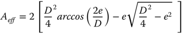
When eccentric loading is considered, a reduction in the foundation area is required; this reduced area is called the effective foundation area. The effective area is defined such that its geometric centre coincides with that of the resultant load. In the case of a circular foundation, the effective area can be calculated from the following formulation:
where:
- Aeff
- Effective foundation area
- (m2)
- D
- Caisson diameter
- (m)
- e
- Eccentric loading point
- (m)
An example of how this reduction would be applied is shown in Figure 5.7. This is recommended in American Petroleum Institute (API) and DNV regulations.
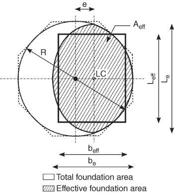
Figure 5.7 Effective foundation area method following Det Norske Veritas (2013).
5.3.1.2 Yield Surface Approach for Bearing Capacity
In the modified bearing capacity factor approach described in the earlier section, each loading condition (V, M, H) is considered separately. However, it is obvious that the capacity of one loading orientation is intrinsically linked to that of the others, as it is the same soil element surrounding the foundation that supports all the three types of loads. Houlsby and Martin (1992) developed an integrated approach for V, M, H loading through the use of plasticity theory. The method is similar to the structural engineering approach (combined axial and bending or the combination of stresses in a material), where a yield surface for an offshore foundation is developed. Research shows that the shape of the yield surface is a rugby ball and is shown in Figure 5.8. Any point in the surface of (V, M, H) space is a yield point, i.e. beyond which plastic deformation will occur.
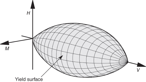
Figure 5.8 Rugby ball failure surface (Source: Villalobos et al. (2009)).
5.3.1.3 Hyper Plasticity Models
The behaviour within the yield surface can be characterised. However, as the load increases on the foundation the yield surface is expected to expand accordingly, and this growth will occur in a plastic manner. To describe this expansion, it is necessary to consider an appropriate strain‐hardening law. Such a theory is known as hyper‐plasticity. To provide a theoretical basis for strain hardening, Gottardi and Houlsby (1995) considered the strain hardening that occurred during a simple load penetration test. These are advanced methods of analysis.
5.3.2 ULS Calculations for Suction Caisson Foundation
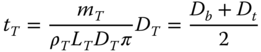
Different variants of suction caissons are considered as suitable foundation and are therefore discussed in more details. The caisson can be considered as a solid embedded object, and under the application of a moment load the caisson will rotate about a single point as a rigid body with or without the bending of the walls/skirts. Apart from moment, the caisson may settle under the vertical load or translate due to lateral load. For preliminary design, often simple analytical methods suffice, and Figure 5.9 shows a generalised sign convention following Butterfield et al. (1997). For mono‐caisson, moment‐carrying capacity is critical and the point of rotation is associated with such calculations. It is often assumed that the point of rotation lies above the foundation level, i.e. within the confines of the caisson skirt. Under the application of a moment load, the deflected shape is described by the rotation of two parallel walls representing the caisson skirt. The rotation of the two parallel walls is such that it is the same as that of the original caisson, as shown in Figure 5.10. The general description of the capacity of a suction caisson has been considered by a number of research groups – Byrne (2000), Villalobos (2006), Schakenda et al. (2011), Cox and Bhattacharya (2017), and Cox (2015) – with the aim of providing a simple method for predicting the ultimate capacity of such a foundation under a series of different loading conditions. Reliable solutions may also be obtained through the use of finite element methods.
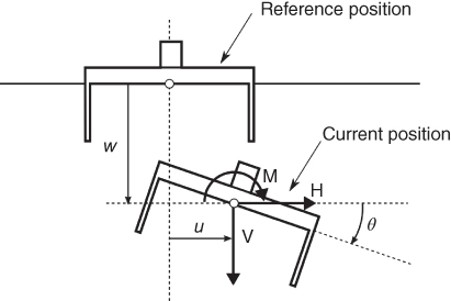
Figure 5.9 Standardised sign convention after Butterfield et al. (1997).
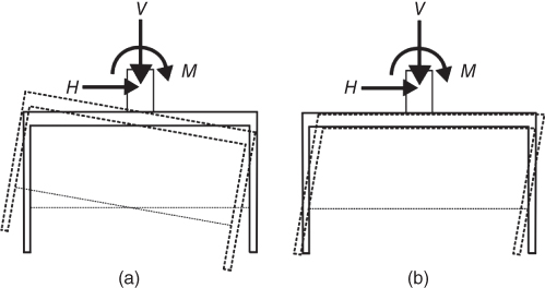
Figure 5.10 Caisson moment loading. (a) true deflection of the caisson; (b) assumed deflection for the purposes of calculation after Schakenda et al. (2011).
5.3.2.1 Vertical Capacity of Suction Caisson Foundations
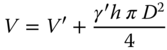
For a typical case, the general bearing capacity equation can be simplified and reduced. This leads to the following equation for a caisson on sand:
where

- Vertical foundation capacity
- (N)
- D
- Caisson diameter
- (m)
It is generally accepted that the general bearing capacity equation (with the reasonable correction factors) models the foundation capacity well. It may be noted that the mobilised angle of friction should be used due to the heaving of the soil plug within the caisson that occurs during installation. Using peak friction angle may lead to an overestimation of capacity. Villalobos (2006) derived empirical calculation for the vertical capacity of a caisson foundation. This is based on the summation of the end‐bearing capacity and skin friction resisting any vertical movement of the caisson:
where:

- Vertical foundation capacity
- (N)

- Effective vertical earth pressure
- (N m−2)
- z
- Foundation depth
- (m)
- kp
- Coefficient of passive soil resistance
- (−)
- ka
- Coefficient of active soil resistance
- (−)
- zm
- Depth to point of caisson rotation
- (−)
- δ
- Soil–structure interface angle of friction
- (°)
5.3.2.2 Tensile Capacity of Suction Caissons
The vertical tensile capacity also needs to be considered if caissons are used in multi‐pod arrangements or as anchors. The tensile capacity of a caisson can be attributed to one of two separate load‐bearing mechanisms. Under a high frequency loading, negative pore pressures and suction may be generated around and within the caisson skirt and is dependent on the speed of loading and the permeability of the surrounding ground. Under low‐frequency loading situations, the tensile capacity will simply be the summation of the frictional components acting on the caisson skirt and the reverse bearing capacity of the foundation. This is further discussed in Example 6.11 of Chapter 6, for example.
5.3.2.3 Horizontal Capacity of Suction Caissons
Generally, the derivation of horizontal capacity of a surface foundation is well agreed upon. The resistance to loading is simply the frictional force generated between the foundation and the supporting soil. This generalised sliding resistance is given by a number of authors in addition to being detailed in DNV regulations (Det Norske Veritas 2013) as follows:
where:
- H
- Horizontal capacity
- (N)
- Aeff
- Effective foundation area
- (m2)
- φ
- Angle of internal friction
- (°)
In the case of an embedded foundation it is reasonable to assume that the additional resistive capacity of the passive soil resistance acting upon the caisson skirt can be considered in addition the frictional resistance already considered. Initially, such a formulation was derived by Byrne (2000) for a suction caisson subjected to a pure horizontal loading, and the capacity of a caisson under such conditions was defined as follows:
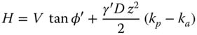
where:
- H
- Horizontal foundation capacity
- (N)
- V
- Vertical foundation capacity
- (N)
- D
- Caisson diameter
- (m)
- z
- Foundation depth
- (m)
- kp
- Coefficient of passive soil resistance
- (−)
- ka
- Coefficient of active soil resistance
- (−)
This formulation was revised by Villalobos (2006) considering the rotation of the foundation at a known depth and is given below.
where:
- α
- Caisson rotational depth (detailed later)
- (m)
For all such cases, the vertical weight is the sum of the buoyant structure and the buoyant weight of the soil contained within the caisson skirt.
From analysis, it is evident that a greater horizontal capacity can be achieved with an increase in the vertical dead weight of the structure.
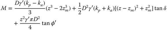
5.3.2.4 Moment Capacity of Suction Caissons
Unlike the derivation of both the vertical and horizontal foundation capacity, there has been a significant amount of debate and analysis over the true definition of the moment capacity of a caisson foundation. All the proposed methods are slightly more complex than its predecessor. Despite the increasing complexity, the difference between the solutions is minimal, and all are suitable for a preliminary estimate. The load‐carrying capacities are estimated based on the lateral earth pressure distribution, skin friction along the walls, eccentric vertical load, and the friction from the underlying slip surface. Using the principle of superposition, the influence of each individual component can be combined to provide a global estimate as to the capacity of the foundation. Figure 5.11 shows the formulation based on Vaitkunaite et al. (2012).
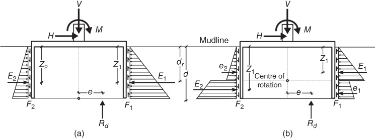
Figure 5.11 Caisson moment capacity as described by (Vaitkunaite et al. 2012). (a) rotation at bottom; (b) rotation at a midpoint.
Considering the two walls separately, the coulomb earth pressure theory can be applied. Using equilibrium, the following calculation concerning the moment capacity of a suction caisson rotation about a point at its base:
or this can be expressed in the form

where:
- M
- Moment wise foundation capacity
- (Nm)
- V, Rd
- Instantaneous vertical foundation capacity
- (m)
- z
- Foundation depth
- (m)

- Effective foundation diameter
- (m)
- kp
- Coulomb coefficient of passive soil resistance
- (−)
- ka
- Coulomb coefficient of active soil resistance
- (−)
- z1
- Depth to passive point of action
- (m)
- z2
- Depth to active point of action
- (m)
This formulation can be evaluated considering a differing depth of rotation. The full derivation and design methodology proposed by Ibsen and MBD offshore power A/S can be found in the patent application filed by Schakenda et al. (2011).
In a similar manner, Villalobos (2006) also considered the effects of a shifting centre of rotation on the moment‐resisting capacity of a suction caisson foundation. Utilising an analysis method similar to that of Ibsen, an alternative formulation for the rotational strength was obtained; see Figure 5.10. Unlike Ibsen, Villalobos included the frictional resistance generated between the soil plug and the surrounding soil mass, see Figure 5.12.
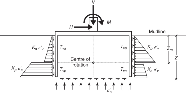
Figure 5.12 Caisson moment capacity as described by Villalobos (2006).
Considering the superposition of each separate variable, the capacity of a suction caisson foundation can be found.
Cox (2014) improved the solution of Villalobos (2006), and the model is presented in Figure 5.13. In the calculations of Villalobos the distribution of vertical earth pressure on the bottom of the caisson was assumed to be even over its area. By considering an eccentricity to the loading profile, it is possible to consider the additional load‐carrying capacity that may be achieved. The frictional effect of shear along the base is still considered and an average load is taken to calculate the friction generated:
Figure 5.13 Caisson moment capacity as described by Cox (2014).
5.3.2.5 Centre of Rotation
Considering the three types of moment formulations proposed, it is clear that a change in the rotation depth can influence the foundation capacity. The effect of a shifting depth of rotation on the capacity of a caisson is considered in Figure 5.14 by taking an example from Cox (2014). The corresponding moment capacity with changing depth of rotation may be noted. For practical purposes, the depth of rotation corresponding to the minimum caisson capacity will be the depth at which the foundation will rotate. This assumes, however, that the rotation will be small and that the active and passive zones are fully developed.
Figure 5.14 Changing moment capacity of theoretical suction caisson based on the moment capacity formulation described by Cox (2014) (D = 12 m, Z = 12 m). Source: Reproduced with permission of PHD Thesis.
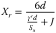
Using the above assumption, Cox (2014) developed a formulation to calculate the depth of rotation for given geometrical and soil parameters. This is essentially based on differentiating the moment equation and finding the minima. The centre of rotation can be calculated using the following equation:
where:

- Vertical foundation capacity
- (N)
- αmin
- Caisson rotational depth at minimum capacity
- (m)
This general calculation indicates that the depth of rotation for a shallow caisson (with a Z/D ratio of 0.5) will be approximately at the base of the caisson and for caissons with a greater aspect ratio the centre of rotation will move proportionally upwards.
5.3.2.6 Caisson Wall Thickness
The thickness of a suction caisson also needs to be designed to resist buckling both during installation and operation. All forces such as the vertical, horizontal, moment, and pressure loads acting on the caisson structure need to be evaluated and appropriately resisted by the caisson structure. Design guidelines are provided in DNV‐OS‐C202 (Det Norske Veritas 2010a) to specify that an appropriate caisson thickness is used to ensure the caisson doesn't buckle.
This standard is generally used industry‐wide for the design of thin‐walled vessels; there has, however, been some discussion on the applicability of these regulations to the design of suction caissons by LeBlanc (2009). This uncertainty is based on the failure of the Wilhelmshaven suction caisson OWT. In this instance, the caisson buckled during installation after it was struck by one of the installation vessels. On subsequent analysis by LeBlanc (2009), it was discovered that minor imperfections in the circularity of a thin‐walled vessel such as a suction caisson can cause the buckling load to be significantly reduced.
5.3.3 ULS Calculations for Pile Design
The ULS calculations for pile foundations needs typically three types of calculations:
- Axial pile capacity (geotechnical): Here the ultimate load corresponds to the failure of the pile whereby the shaft resistance and the end‐bearing resistance is fully mobilised and the pile fails in excessive settlement. Typically, if the axial pile‐head displacement is more than 10% of the pile diameter, it may be considered that the ultimate capacity is reached. The parameters that are needed are soil parameters (typically strength parameters) and the geometry of the pile (length, diameter, and wall thickness).
- Axial pile capacity (structural): If the pile is laterally unsupported due to excessive scour in the upper depths or soil layers momentarily liquefying due to earthquake, it may buckle (Euler type global buckling). This must be considered in seismic areas. Long, slender thin‐walled piles are particularly vulnerable.
- Structural capacity of the section (plastic moment capacity, MP as well as moment at first yield, MY): This shows the maximum moment that the pile section can carry before the material of the pile yields. This is a function of the pile geometry (diameter, wall thickness) and material properties (yield strength). An example problem is shown in Chapter 6 (Example 6.11).
- Moment‐carrying capacity of the pile (geotechnical). This is important for monopile design, and in this condition, the soils surrounding the pile fails.
5.3.3.1 Axial Pile Capacity (Geotechnical)
The failure load or ultimate load of a pile is the summation of shaft resistance (also known as skin friction or side friction) along the embedded length of a pile and end‐bearing at the pile toe. Mathematically, the side friction is the integral of the shear stress over the cylindrical surface of the pile, and the end bearing is the integral of the normal stress on the pile tip. Most, if not all, offshore piles are thin‐walled steel section, and they may be closed‐ended (also known as plugged) or open‐ended (also known as unplugged). For closed‐ended pile, the pile drives as if it is solid section, and therefore there are two terms: end bearing of the whole area of the pile and side friction of the outer pile surface. On the other hand, for open‐ended conditions, the pile cuts around a plug of soil and the plug remains almost static in the ground. In this case, there are three terms: end bearing of the annulus of the section, side friction of the outer pile surface, and side friction in the inner pile surface. Figure 5.15 shows one particular case.
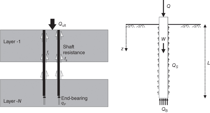
Figure 5.15 Static capacity of a pile (unplugged condition) and plugged condition.
It is very difficult to ascertain whether a pile will behave plugged or unplugged (Figure 5.15). Therefore, a pragmatic approach is taken in most codes of practices whereby axial capacity is considered for two cases and the lower of the two is taken.
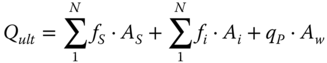
Axial capacity: open‐ended pipe pile and the capacity is given by Eq. (5.16):
where:
- Qult
- =
- Ultimate static capacity
- fs
- =
- Unit outside shaft friction
- As
- =
- Outside shaft area of pile
- fi
- =
- Unit inside shaft friction
- Ai
- =
- Inside shaft area of pile
- qp
- =
- Unit end bearing capacity
- Aw
- =
- Cross‐sectional area of steel wall at toe of pile
- N
- =
- Number of layers
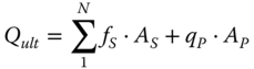
The capacity of the closed‐ended pile is given by Eq. (5.17):
where:
- Ap
- =
- Gross end‐bearing area
There are different methods to estimate the capacity and the notable ones are: API, NGI, Fugro, UWA (University of Western Australia) and ICP (Imperial College Pile) method.
API method is widely used for small‐diameter piles and the parameters can be obtained from soil testing and site investigation. The following are from the twenty‐first edition of the API‐RP2A – WSD 2000 method (RP stands for Recommended Practice, WSD stands for working stress design). The readers are referred to the latest codes of practice or best practice guide for such purpose. However, the fundamentals of the calculations remains the same.
- Parameters for sandy soil (Coarse grained soil) – API approach (Table 5.1)
- Unit shaft friction
where:
- K
- =
- Coefficient of lateral earth pressure

- =
- Effective overburden pressure at the point in question
- δ
- =
- Angle of friction between soil and pile wall
- Unit end bearing
where:
- Nq
- =
- Bearing capacity factor for deep foundation [See later on]

- =
- Effective overburden pressure at the pile tip
- Parameters for clayey soil (fine grained soil) – API approach
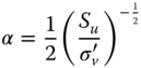
- Unit shaft friction
where:
- α
- =
- A dimensionless factor, derived as outlined below
- Su
- =
- Undrained shear strength of the soil at the point in question
- Unit end bearing
API (2000) method, suggests the following:
- Case 1:
For ![]()
- Case 2:
For ![]()

For simplified calculations, it may be assumed that equal shaft resistance acts at the inside and outside of open‐ended piles. There are excellent text books where the axial capacity of a pile is dealt with in great detail. One such is Randolph and Gourvenec (2011).
Table 5.1 Design parameters for coarse‐grained soila from API.
| Density | Soil type | Soil‐pile friction angle (Degrees) | Limiting friction (kPa) | Nq | Limiting end bearing (MPa) |
|
Very Loose Loose Medium |
Sand Sand‐Siltb Silt |
15 | 47.8 | 8 | 1.9 |
|
Loose Medium Dense |
Sand Sand‐Silt b Silt |
20 | 67.0 | 12 | 2.9 |
|
Medium Dense |
Sand Sand‐Silt b |
25 | 81.3 | 20 | 4.8 |
|
Dense Very Dense |
Sand Sand‐Silt b |
30 | 95.7 | 40 | 9.6 |
|
Dense Very Dense |
Gravel Sand |
35 | 114.8 | 50 | 12.0 |
aWhere detailed information such as in‐situ cone tests is available, values and limits may be modified.
bSand‐Silt fractions – strength values generally increase with increasing sand fraction.
5.3.3.2 Axial Capacity of the Pile (Structural)
The allowable axial load in terms of buckling instability depends on the following:
- Length of the pile likely to be unsupported due to scour and liquefaction
- Boundary condition of the pile below and above the unsupported zone
- Bending stiffness of the pile (EI)
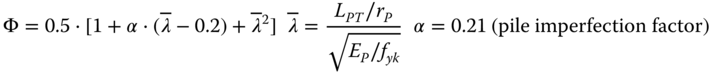
Basic Euler equation may be used. The readers are referred to the paper by Bhattacharya et al. (2005).
Where ![]() is the normalised unsupported length (L) of the pile.
is the normalised unsupported length (L) of the pile. ![]() is L for fixed headed pile (i.e. typical jacket pile). On the other hand, for free‐headed pile (i.e. monopile)
is L for fixed headed pile (i.e. typical jacket pile). On the other hand, for free‐headed pile (i.e. monopile) ![]() is 2L.
is 2L.
The unsupported length of the pile (L) can be estimated by the adding three terms: Scour depth + Liquefiable zone depth + Depth of fixity at the bottom of the unsupported length of the pile. In the absence of detailed investigation, this can be taken as three times the diameter of the pile. The readers are referred to Bhattacharya and Goda (2013) for details of the calculations.
5.3.3.3 Structural Sections of the Pile
Methods to obtain plastic moment capacity (MP) and moment at first yield (MY) are provided in Example 6.10 of Chapter 6 . Furthermore, the pile section has to be checked for general and local buckling, and this section provides guidelines in this respect. Based on the methods described in Chapter 2, one can calculate the total bending moment by assuming collinear wind and waves. This is by summing the bending moments due to each, and applying an environmental load factor γL = 1.35 as prescribed in (DNV 2010a,b).
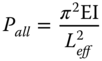
The ULS depends on the length of the pile, as it determines whether the monopile or the soil will fail first. A simplified methodology proposed in (Poulos and Davis 1980) recommends that for practical parameter sets, the pile fails first through yielding. The ultimate overturning moment the pile can carry is then calculated simply by:

where fy = 355 MPa is the pile material's yield strength. With this the pile can take the maximum load if Mγ < My.
General and Local Buckling
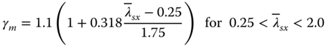
For bar buckling under compression and bending moment, the Germanischer Lloyd (2005) code prescribes the following formula:
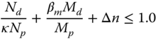
where Nd is the design axial force, κ is the reduction factor for bar buckling, Np is the plastic compression resistance, βm is the moment coefficient for bar buckling, Md is the design bending moment, Mp = Wpfy/γM is the plastic moment resistance with Wp being the plastic section modulus and γM = 1.1 the material safety factor. The following equations can be used to calculate each term. (For the meaning of symbols, please refer to the nomenclature as well as the code.)

where:
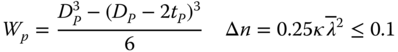
Local (shell) buckling needs to be checked as well, and according to Germanischer Lloyd (2005) the following formula can be used
where σϕ is the design circumferential (hoop) stress, σϕu is the ultimate circumferential stress for shell buckling, σx is the design axial stress, and σxu is the ultimate axial stress for buckling. The following equations can be used to calculate each term. The ultimate shell buckling stress for axial stress is

where κ2 = 1.0 for ![]() ,
, ![]() for
for ![]() ,
, ![]() for
for ![]() , and
, and ![]() for
for ![]() , with
, with ![]() and σxi is the ideal buckling stress for axial stress:
and σxi is the ideal buckling stress for axial stress:
with
η = 1 for both ends simply supported, η = 3 for one end simply supported, one end clamped, η = 6 for both ends clamped. The safety factor can be calculated according to the following:
The ultimate shell‐buckling stress for circumferential stress is
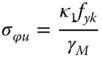
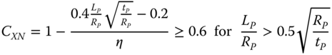
where κ1 = 1.0 for ![]() ,
, ![]() for
for ![]() ,
, ![]() for
for ![]() with
with ![]() . The ideal buckling stress for circumferential stress is
. The ideal buckling stress for circumferential stress is

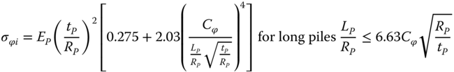
where Cϕ = 1.5 for both ends clamped, Cϕ = 1.25 for one end simply supported, one end clamped, Cϕ = 1.0 for both ends simply supported, Cϕ = 0.6 for one end clamped, one end free. The material safety factor is γM = 1.1.
5.3.3.4 Lateral Pile Capacity
For long‐term deformation production, moment carrying capacity needs to be estimated. There are many methods to carry out such calculations: simplified method (hand‐based method), standard method (Beam on Winkler Foundation – discussed later in this chapter) or finite element method. This section presents one simplified method based on Broms (1964) approach. For derivation and details, please refer to Chapter 7 of Poulos and Davis (1980).
Constant Soil Resistance with Depth
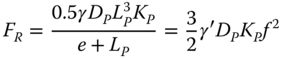
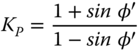
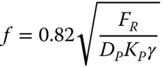
In ground conditions where the soil resistance is assumed to be constant with depth (OCR soils), and where soil fails first (i.e. the pile does not fail through a plastic hinge formation), the ultimate capacity can be calculated using the following formulae.


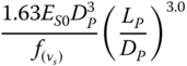
where su is the undrained shear strength, e is the eccentricity of loading, MR is the moment capacity of the pile, FR is the horizontal load carrying capacity of the pile, DP and LP are the diameter and embedded length of the pile, respectively (Figure 5.16).
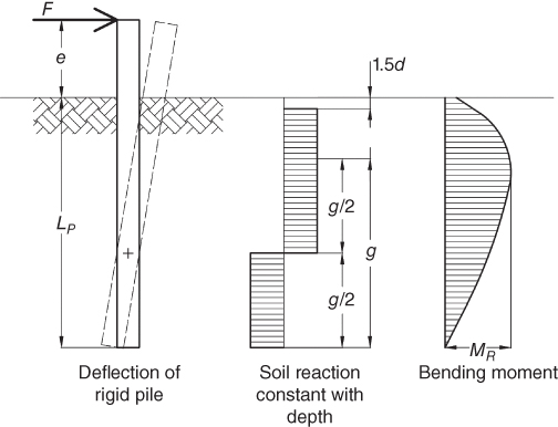
Figure 5.16 Lateral capacity for pile with ground stiffness constant with depth.
Linear Soil Resistance with Depth
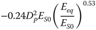
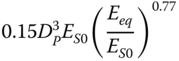
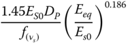
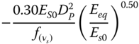
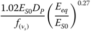
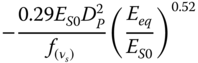
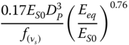
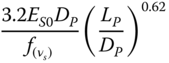
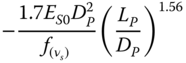
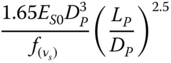
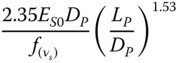
In ground conditions, where the soil resistance is assumed to increase linearly with depth (e.g. some cohesionless soils and lightly overconsolidated clay), the horizontal load and moment capacity of a piled foundation, assuming that the soil fails first (no plastic hinge is formed in the pile), is expressed using the following equations (Figure 5.17):
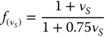
where ![]() is the submerged unit weight of the cohesionless soil (assumed constant with depth); DP and LP are the pile diameter and embedded length, respectively; e is the load eccentricity (e = M/F);
is the submerged unit weight of the cohesionless soil (assumed constant with depth); DP and LP are the pile diameter and embedded length, respectively; e is the load eccentricity (e = M/F); ![]() is the effective angle of internal friction; and MR and FR are the moment and the horizontal load carrying capacity of the foundation, respectively. For derivation and details, refer to Chapter 7 of Poulos and Davis (1980).
is the effective angle of internal friction; and MR and FR are the moment and the horizontal load carrying capacity of the foundation, respectively. For derivation and details, refer to Chapter 7 of Poulos and Davis (1980).
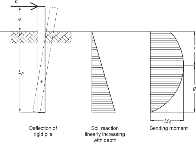
Figure 5.17 Lateral pile capacity with ground stiffness increasing linearly with depth.
5.4 Methods of Analysis for SLS, Natural Frequency Estimate, and FLS
There are different approaches to incorporate the effects of SSI. In the context of OWT design, this can be classified into three categories as shown in Table 5.2.
Table 5.2 Methods of SSI analysis.
| Simplified | Standard | Advanced | |
| Details of the method | In this method, the foundation is replaced by a set of springs: KL, KR, and KLR. Therefore, the model is similar to a beam supported on a set of non‐linear springs. Figure 5.18 explains the method. If spreadsheets are developed, this method takes about 10 min to carry out the calculations. | This method is based on Beam on nonlinear Winkler foundations. The pile–soil interaction or the foundation soil interaction is modelled as a series of nonlinear springs. This method is not expensive in terms of computation and does not need specialist geotechnical knowledge. |
This method is based on advanced numerical analysis and the possible methods are finite element, finite difference, discrete element. Finite element is most commonly used in practice and expertise is necessary. The readers are referred to Potts (2013) Rankine Lecture |
| What are the ground parameters required? | Two parameters are required:
|
The parameters needed are stress–strain of soils (i.e. some form of soil shear tests preferably triaxial tests). Some formulations may need Subgrade modulus data and relative density of the soil. These are routine soil tests. |
Soil parameters depending on soil models. |
| What this method can do? | This method can predict the natural frequency of the system using the formulation presented in Arany et al. (2016). The method can also predict the deformation of the pile head. | This method can be used to obtain foundation stiffness which can be then be used for structural/dynamic analysis. Bending moment and deflection profile along the length of the pile can also be obtained. | FE model can be used to obtain foundation stiffness, deflection, and moment in the pile. The method can also estimate the strain field in the soil in the deformed/mobilised zone. |
| Limitation of the method | Cannot produce a bending moment and deflection profile of the pile | The pile–soil interactions are modelled as a series of discrete springs. However, in reality, the springs are not independent. | This is very expensive and needs trained personnel. |
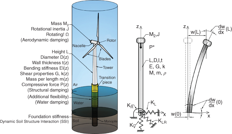
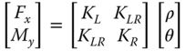
Figure 5.18 Simplified model for SSI analysis.
5.4.1 Simplified Method of Analysis
In a simplified method of analysis, the following steps may be adopted:
- To find the loads on the foundation for various load combinations. For a monopile or a mono‐caisson type foundation, this would mean obtaining vertical load, overturning moment (My), and horizontal load (Fx).
- The second step is to choose a foundation and obtain the stiffness values, denoted by KL, KR, and KLR in Figure 5.7. The stiffness can be obtained in a variety of ways. The simplest is based on closed‐form solutions that need only a few parameters: pile dimensions, Young's modulus of soil at a depth of one pile diameter, and variation of soil stiffness with depth. Tables 5.3 and 5.4 provide closed‐form solution for stiffness for rigid piles and flexible piles. Other methods such as Winkler‐type solution (i.e. referred to as standard method and discussed in Section 5.4.3) or finite element method (referred to as the advanced method and discussed in Section 5.4.4) may also be used to obtain stiffness values. The foundation stiffness is required for two calculations: deformation (deflection ρ and rotation θ at mudline) and natural frequency estimation. A few points may be noted regarding these springs:
- The properties and shape of the springs (load‐deformation characteristics, i.e. lateral load‐deflection or moment‐rotation) should be such that the deformation is acceptable under the working load scenarios expected in the lifetime of the turbine.
- The initial values of the springs (stiffness of the foundation) are necessary to compute the natural period of the structure using linear Eigen value analysis.
- The values of the springs will also dictate the overall dynamic stability of the system due to its nonlinear nature. It must be mentioned that these springs are not only frequency dependent but also change with cycles of loading due to dynamic soil–structure interaction.
- Once the stiffness values KL, KR, and KLR are estimated, deformations in the foundation can be estimated using Eq. (5.38) assuming linearity in load deformation relationship:
5.38where Fx is the lateral force in the direction of the x‐axis as defined in Figure 5.18, My is the fore–aft overturning moment (around the y‐axis), KL is the lateral spring, KR is the rotational spring, KLR is the cross‐coupling spring, ρ is the displacement in the x direction, and θ = ∂ρ/∂z is the slope of the deflection (tilt or rotation).
The deformations can then be easily expressed using (Figure 5.18)
5.39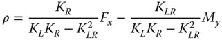 5.40
5.40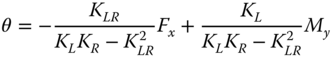
- The natural frequency of the system shown in Figure 5.18 can be estimated following method developed in Arany et al. (2015b, 2017). This simplified methodology builds on the simple cantilever beam formula to estimate the natural frequency of the tower, and then applies modifying coefficients to take into account the flexibility of the foundation and the substructure. This is expressed as:
5.41where CL and CR are the lateral and rotational foundation flexibility coefficients, CS is the substructure flexibility coefficient and fFB is the fixed‐base (cantilever) natural frequency of the tower. The readers are referred to Appendices.
Table 5.3 Stiffness formulae by different researchers for slender piles in various soil profiles.
| Lateral stiffness KL | Cross-coupling stiffness KLR | Rotational stiffness KR |
| Randolph (1981), slender piles, both for homogeneous and linear inhomogeneous soils | ||
 |
 |
 |
| Pender (1993), slender piles, homogeneous soil | ||
 |
 |
 |
| Pender (1993), slender piles, linear inhomogeneous soil | ||
 |
 |
 |
| Pender (1993), slender piles, parabolic inhomogeneous soil | ||
 |
 |
 |
| Poulos and Davis (1980) following Barber (1953), slender pile, homogeneous soil | ||
 |
||
| Poulos and Davis (1980) following Barber (1953), slender pile, linear inhomogeneous soil | ||
| Gazetas (1984) and Eurocode 8 Part 5 (2003), slender pile, homogeneous soil | ||
 |
 |
 |
| Gazetas (1984) and Eurocode 8 Part 5 (2003), slender pile, linear inhomogeneous soil | ||
 |
 |
 |
| Gazetas (1984) and Eurocode 8 Part 5 (2003), slender pile, parabolic inhomogeneous soil | ||
 |
 |
 |
| Shadlou and Bhattacharya (2016a), slender pile, homogeneous soil | ||
 |
 |
 |
| Shadlou and Bhattacharya (2016a), slender pile, linear inhomogeneous soil | ||
 |
 |  |
| Shadlou and Bhattacharya (2016a), slender pile, parabolic inhomogeneous soil | ||
 |
 |
 |
| Parameter definitions: | ||

 for Randolph (
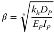
Table 5.4 Stiffness formulae by different researchers for rigid piles in various soil profiles.
| KL | KLR | KR |
| Poulos and Davis (1980) following Barber (1953), rigid pile, homogeneous soil (n = 0) | ||
| khDPLP |  |
 |
| Poulos and Davis (1980) following Barber (1953), rigid pile, linear inhomogeneous soil (n = 1) | ||
| Carter and Kulhawy (1992), rigid pile, rock | ||
 |
 |
 |
| Shadlou and Bhattacharya (2016a), rigid pile, homogeneous soil (n = 0) | ||
 |
 |
 |
| Shadlou and Bhattacharya (2016a), rigid pile, linear inhomogeneous soil (n = 1) | ||
 |
 |
 |
| Shadlou and Bhattacharya (2016a), rigid pile, parabolic inhomogeneous soil (n = 1/2) | ||
 |
 |
 |
| Parameter definitions: | ||
 |
 |
|
The fixed‐base natural frequency of the tower is expressed simply with the equivalent stiffness k0 and equivalent mass m0 of the first mode of vibration as
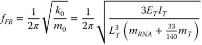
where ET is the Young's modulus of the tower material, IT is the average area moment of inertia of the tower, mT is the mass of the tower, mRNA is the mass of the rotor‐nacelle assembly and LT is the length of the tower. The average area moment of inertia is calculated as
where Db is the tower bottom diameter, Dt is the tower top diameter. The average wall thickness and the average tower diameter are given by Eq. (5.44).
where ρT is the density of the tower material (steel). The coefficients CL and CR are expressed in terms of the nondimensional foundation stiffness values:
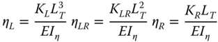
where KL, KLR, KR are the stiffness parameters, EIη is the equivalent bending stiffness of the tower calculated as

The derivation of the above equations are provided in Appendices A to C.
Using the calculated nondimensional stiffness values, the foundation flexibility coefficients are given as
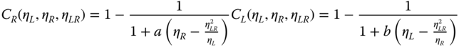
where a = 0.5 and b = 0.6 are empirical coefficients (Arany et al. 2016, 2017).
The substructure flexibility coefficient is calculated by assuming that the monopile goes up to the bottom of the tower. The distance between the mudline and the bottom of the tower is LS, and EPIP is the bending stiffness of the monopile. The foundation flexibility is expressed in terms of two dimensionless parameters, the bending stiffness ratio χ and the length ratio ψ
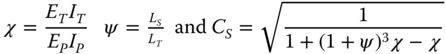
A spreadsheet can be easily used to carry out the calculations. A solved example is carried out in Chapter 6 . This method is calibrated for 10 offshore wind turbines and can be found in Arany et al. (2016).
5.4.2 Methodology for Fatigue Life Estimation
The analysis of fatigue life of the substructure has to be carried out, which is typically done following DNV‐RP‐C203 – ‘Fatigue design of offshore steel structures’ (DNV 2005). This section is aimed at providing a simple methodology for the conceptual design of monopiles, and therefore fatigue life issues related to other components of the substructure (e.g. transition piece, grouted connection, J‐tubes, etc.) are naturally omitted. In terms of fatigue analysis of the structural steel of the pile wall under bending moment, one has to calculate the stress levels caused by various load cases. The material factor γM = 1.1 and load factor γL = 1.0 can be used.
With these, the maximum stress levels σm caused by the load cases can be calculated as
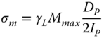
where Mmax is the maximum bending moment that occurs in the given load case, DP and IP are the pile diameter and area moment of inertia, respectively. The maximum cyclic stress amplitude is given as
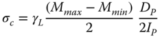
where Mmin is the lowest bending moment occurring in each of the load cases.
In typical practical cases, the fatigue analysis of the structural steel of a monopile results in sufficient fatigue life with a high margin. However, the welds of flush ground monopiles are more prone to fatigue‐type failure, as fatigue crack initiation typically occurs around the welds before it would occur in the structural steel. The fatigue analysis of welds of flush ground monopiles is carried out using the C1 and D classes defined in DNV (2005). A thickness correction factor has to be applied as monopile welds are almost always thicker than 25 mm. These curves build on tests carried out specifically for the requirements of the offshore oil and gas (O&G) industry. Currently, research and testing are ongoing in the SLIC Joint Industry Project (Brennan and Tavares 2014) to develop S–N curves representative of the load regime, geometry, materials, environmental conditions, and manufacturing procedures of the offshore wind industry. More detailed fatigue analyses through, e.g. finite element analysis (FEA) may need to be carried out once a more detailed design is available, as fatigue‐type failure is expected to occur in weak points in the structure (e.g. holes, welds, and joints) where stress concentration is expected and crack initiation is more likely. Furthermore, a crack propagation approach is generally more suitable for detailed fatigue design and simple S–N curve fatigue analyses are often not satisfactory to predict the fatigue life of certain structural details.
5.4.3 Closed‐Form Solution for Obtaining Foundation Stiffness of Monopiles and Caissons
In a simplified three‐springs approach (see Figure 5.8), foundation stiffness needs to be calculated. They are: KV (vertical stiffness), KL (lateral stiffness), KR (rocking stiffness), and KLR (cross‐coupling). It is required to note that the vertical stiffness is not required for simplified calculations as the structure is very stiff vertically. However, values of KV are required for rocking modes of vibration. In a simplified approach or a closed‐form solution approach, the input required to obtain KL, KR, and KR are:
- Pile dimensions.
- Ground profile, i.e. soil stiffness variation with depth. In line with Eurocode practice (EC8, Part 5), three types of profiles are considered. They are: (i) constant stiffness with depth which is typical of overconsolidated clay profile; (ii) linearly varying stiffness with depth which is typical of normally consolidated (NC) clay; and (iii) soil stiffness varying with square root of depth, which is typical of sandy soil. Figure 5.8 plots the variation.
- Soil stiffness at a depth of one pile diameter.
Alternatively, some formulations define the soil with the modulus of subgrade reaction kh or the coefficient of subgrade reaction nh (the rate of increase of kh with depth).
Note: Terminologies such as subgrade modulus, coefficient can be confusing. Codes of practices, textbooks, and software require different types of inputs. It is therefore recommended to always write units.
5.4.3.1 Closed‐Form Solution for Piles (Rigid Piles or Monopiles)
The first step in the calculation procedure of the pile‐head stiffness is the classification of pile behaviour, i.e. whether the monopile will behave as a long flexible pile or a short rigid pile, and then using the appropriate relations to obtain KL, KR, and KLR.
Rigid piles are short enough to undergo rigid body rotation in the soil under operational loads, instead of deflecting like a clamped beam. Slender piles, on the other hand, undergo deflection under operating loads and fail typically through the formation of a plastic hinge, and the pile toe does not ‘feel’ the effects of the loading at the mudline and the pile can be considered infinitely long. Formulae for determining whether a pile can be considered slender or rigid are available in the literature. Calibrated method for natural frequency estimate by Arany et al. (2016) suggests the following.
Flexible Behaviour or Rigid?
Based on the elastic continuum approach proposed by Randolph (1981), the critical pile length can be expressed through the necessary ratio of pile length LP to pile diameter DP in terms of the modified shear modulus G* of the soil and the equivalent Young's modulus of the pile (Eeq). With this the pile length is calculated from the diameter as

where ![]() ,
, ![]() with GS being the shear modulus of the soil averaged between the mudline and the pile embedment length, EPIP is the pile's bending stiffness.
with GS being the shear modulus of the soil averaged between the mudline and the pile embedment length, EPIP is the pile's bending stiffness.
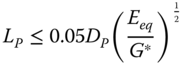
Carter and Kulhawy (1992) present an expression to determine whether the pile can be considered rigid using a similar approach to that of Randolph (1981) whereby the pile is rigid if
Another approach is shown in Poulos and Davis (1980) following Barber (1953) using the soil's modulus of subgrade reaction kh. In cohesive soils (which applies to the overconsolidated clayey ground profile), the modulus of subgrade reaction kh can be considered constant with depth. The pile can be considered slender (infinitely long) if
and the pile can be considered rigid if
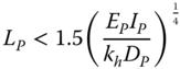
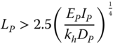
In normally consolidated clay or cohesionless soils (sand), the modulus of subgrade reaction approximately increases linearly with depth, according to kh = nh(z/DP). In such soils the pile can be considered slender if
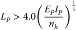
and the pile can be considered rigid if

These formulae can be used to obtain the necessary length as a function of pile diameter and soil stiffness.
Other methods to find critical length can be found in Aissa et al. (2017).
In the simplified procedure to obtain foundation stiffness, two parameters are required to define the ground (soil stiffness at 1DP below mudline denoted by ES0 and the stiffness profile, i.e. variation with depth). The stiffness profile is expressed mathematically as
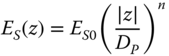
where homogeneous, linear inhomogeneous, and square root inhomogeneous profiles are given by n = 0, n = 1, and n = 1/2, respectively (see Figure 5.19).
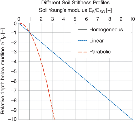
Figure 5.19 Homogeneous, linear, and parabolic soil stiffness profiles.
Analytical solutions are rarely available from a subgrade approach for general cases, but simplified expressions are available for rigid and slender piles and available in (Poulos and Davis 1980). Various approaches have been developed to correlate foundation loads (horizontal load Fx and bending moment My) to pile‐head deflection ρ and rotation θ. These expressions can be easily transformed into a matrix form of the load response in terms of three springs (KL, KLR, KR). Some of the most common methods are found in Poulos and Davis (1980) following Barber (1953) for both rigid and slender piles; Gazetas (1984) also featured in Eurocode 8 Part 5 (European Committee for Standardization 2003) developed for slender piles; Randolph (1981) developed for slender piles in both homogeneous and linear inhomogeneous soils; Pender (1993) developed for slender piles; Carter and Kulhawy (1992) for rigid piles in rock; Higgins and Basu (2011) for rigid piles; and Shadlou and Bhattacharya (2016a) for both rigid and slender piles. The formulae for the foundation stiffness are summarised in Table 5.3 for slender piles and Table 5.4 for rigid piles (Figure 5.20).
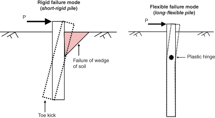
Figure 5.20 Distinguishing failure between short‐rigid pile and long flexible pile.
5.4.3.2 Closed‐Form Solutions for Suction Caissons
Shadlou and Bhattacharya (2016a) presented impedance functions for rigid deep foundations in homogeneous, parabolic, and linear ground profiles, keeping in mind the application for offshore wind turbines. Table 5.5 presents solutions that are applicable for L/D greater than 2. The definition of L and D are given in Figure 5.21. Jabli et al. (2018) presented solutions for stiffness of suction caissons having rigid skirted for 0.5 < L/D < 2 in three types of ground profiles for Table 5.5, (L/D > 2) see Table 5.6 for Table 5.6 for 0.5 < L/D < 2. An example problem is carried out in Chapter 6 to show the application. The variation of Poisson's ratio may be noted for two types of aspect ratio (Figure 5.21).
Note: It must be mentioned that these solutions can be used for preliminary sizing of caisson at feasibility and tender design stage. Once the size is optimised and the project is finalised, further optimization and detailed analysis should be carried out using conventional methods.
Table 5.5 Impedance functions for section caissons exhibiting rigid behaviour L/D > 2. See Figure 5.21.
| Ground profile See Figure 5.19 for definition |  |
 |
 |
| Homogeneous | |||
| Parabolic | |||
| Linear |
Figure 5.21 Definition of the suction caissons.
Table 5.6 Impedance functions for shallow‐skirted foundations exhibiting rigid behaviour 0.5 < L/D < 2.
| Ground profile |  |
 |
 |
| Homogeneous | |||
| Parabolic | |||
| Linear |
The value of ![]() is given by the equation in Section 5.4.3.2.
is given by the equation in Section 5.4.3.2.
5.4.3.3 Vertical Stiffness of Foundations (KV)
Rigid Circular Embedded Footings
The (DNV 2002) provides guidance for rigid embedded shallow foundations over a bedrock layer and may be used as a preliminary estimate for suction caissons (Figure 5.22).

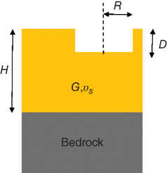
Figure 5.22 Figure defining the terms in Eq. (5.58).
Vertical Stiffness of Piles
Fleming et al. (1992) suggested the following for embedded piles:
Shaft friction only**
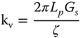
ζ is between 3 and 5
LRFD guidelines for seismic design of bridge propose the following relation for vertical stiffness (Sharma and El Naggar 2015):
Note: In practice, t‐z (axial load transfer analysis) type of analysis or calibrated FEA can be carried out to obtain the axial stiffness of the piles.
5.4.4 Standard Method of Analysis (Beam on Nonlinear Winkler Foundation) or p‐y Method
To model laterally loaded piles, practicing engineers often use a simplified method normally referred to as Beam‐on‐Nonlinear‐Winkler‐Foundation BNWF) following Winkler (1867a,b) and Hetényi (1946). This is often known as p‐y method and the main hypothesis is that the soil reaction p, exerted by the soil at a certain elevation on the pile shaft, is proportional to the relative pile‐soil deflection, y. In offshore O&G industry, p‐y method is employed to find out pile‐head deformations (deflection and rotation) and foundation stiffness. The approach can be found in API (2005) and also suggested in DNV (2014). Originally, it was developed by Matlock (1970a,b); Reese et al. (1975); O'Neill and Murchinson (1983). The basis of this methodology is the Winkler approach (Winkler 1867a,b) whereby the pile–soil interaction is modelled as independent springs along the length of the pile. The well‐known limitation of this method is the independent nature of these springs. However, it has been successfully used in O&G industry for more than 40 years.
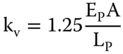
According to the BNWF method, the pile is modelled by means of consecutive beam‐column elements, whereas the LPSI (Lateral Pile Soil Interaction) is modelled through nonlinear springs attached to nodal points between two consecutive elements; see Figure 5.23. Each spring is defined by means of a nonlinear relationship between soil reaction per unit length of the pile p and corresponding relative soil–pile horizontal displacement, y. The coefficient of proportionality between p and y is the modulus of subgrade reaction k, with dimension of pressure divided by length. This relationship is normally referred to as p‐y curve or soil‐reaction curve. Intuitively, p‐y curves depend on the soil and the pile diameter as it is effectively bearing capacity problem in the lateral direction whereby the pile section pushes the soil. Figure 5.23 shows a BNWF model for two types of p‐y curves (two extremes), and it is important to highlight the importance of the shape of these curves.
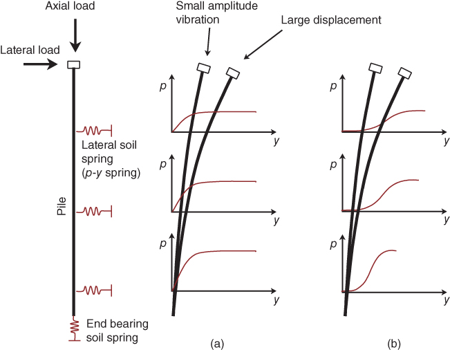
Figure 5.23 Winkler model showing pile response resulting from two types of p‐y curves: (a) strain‐softening response soils; (b) strain‐hardening response.
- The first case (5.23a) is representative of strain‐softening behaviour. This type of behaviour is typical of most soils, i.e. sand or clay.
- The second case is representative of strain‐hardening behaviour exhibited by post‐liquefied soils. Once soil liquefies (i.e. effective stress is zero), the strength and stiffness reduce to zero and the p‐y curve is aligned along the y‐axis – the micromechanics being the soil grain particles are not in contact. However, with pile–soil relative displacement, the grains start to interlock and we note a strain‐hardening behaviour.
This directly obtained results of the p‐y model or its derivative is used for two types of calculations for offshore wind turbines:
- Natural frequency estimate (i.e. eigen value problem which by definition is linear) requires stiffness of the pile for small amplitude vibrations. In this case, the behaviour that is of interest is the stiffness of the pile at very small pile displacement, which will lead to stiffness of the soil at very small strains. This is depicted in Figure 5.23a,b. Therefore, small strain stiffness measurement is very important and the readers are referred to the discussion in Chapter 4.
- On the other hand, if the behaviour of the pile is required to be modelled for storm loading or ultimate behaviour, the behaviour of the soil at large strain is of interest.
Figure 5.23 schematically illustrates the effects of different shapes of p‐y curve. For concave‐downward strain‐softening p‐y curve illustrated in Figure 5.23a, it can be noted that when the relative soil–pile displacement is small, the resistance experienced by the pile depends on the initial stiffness of the soil and corresponding value of deflection. For large displacement, however, the resistance offered by the adjacent soil is governed by the ultimate strength of the soil.
In contrast, if the shape of the p‐y curve is concave‐upward, i.e. strain‐hardening, the pile response is much more complex and may be significantly different from that described above. In seismic zones, if the top layer liquefies, owing to the practically zero stiffness mobilised at small displacements, the soil may offer minimal opposition to any lateral movement of the pile. This will result in enhanced P‐delta moment and in extreme scenarios, buckling mode of failure of the pile. On the other hand, the higher stiffness and strength mobilised at larger displacements may prevent a complete collapse of the structure.
5.4.4.1 Advantage of p‐y Method, and Why This Method Works
Despite its limitations of discrete nature, i.e. the springs work independently, the BNWF method is extensively used in practice because of its mathematical convenience and ability to incorporate nonlinearity of the soil and ground stratification. For example, in the closed‐form method or solutions presented in Section 5.4.3 and Tables 5.5 and 5.6, only three types of profile could be modelled. On the other hand, using the BNWF method, any type of stratification could be modelled. The validity of BNWF approach is based on the assumed similarity between two mechanical system responses:
- Load‐deformation response of the pile, which takes into account the overall macro behaviour of the soil–pile system.
- Stress–strain response of the adjacent soil being sheared as the pile moves laterally. This is related to the micro behaviour of the deforming material.
In theory, the transformation from micro (stress–strain of the soil) to macro (p‐y curves) can be made by applying appropriate scaling factors, whereby stress is converted into equivalent soil reaction, p; and strain is converted into equivalent relative pile‐soil displacement (y). Dash (2010), Bouzid et al. (2013) demonstrated that appropriate scaling factors can be derived from the so‐called mobilisable strength design (MSD) method. Essentially, any stress–strain curve of a soil can be used to construct a p‐y curve through scaling and this method is gaining popularity. Lombardi et al. (2017) and Dash et al. (2017) developed p‐y curves of liquefied soil from the stress–strain data of liquefied soil based on the scaling method developed by Bouzid et al. (2013). This method is discussed later in this chapter and is known as scaling method (Figure 5.24).
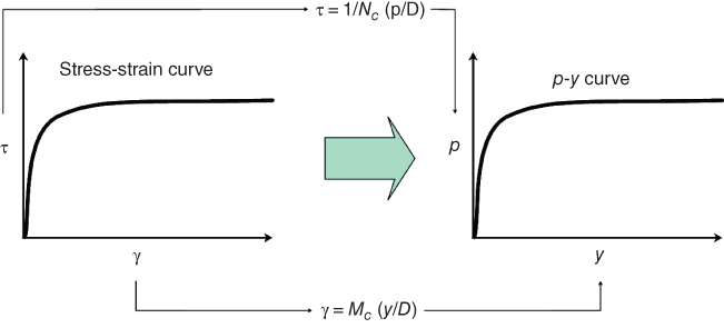
Figure 5.24 Scaling method for obtaining p‐y curve from stress–strain behaviour. Note MS and NS are the scaling coefficients to convert the stress–strain to p‐y.
5.4.4.2 API Recommended p‐y Curves for Standard Soils
The p‐y curves are constructed by means of empirical relationships and were originally developed in the 1970–1980s from a relatively limited number of full‐scale tests carried out on flexible steel piles (Matlock 1970a,b; Reese et al. 1974; Reese et al. 1975; O'Neill and Murchison 1983). Table 5.7 provides details of the reference of the research on which API p‐y curves are based.
5.4.4.3 p‐y Curves for Sand Based on API
For sand: The p‐y curve for a pile in sand is generated using the following derivation;
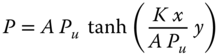
where:
- A
- Cyclic loading parameter
- (−)
- Pu
- Ultimate lateral resistance
- (kN m−1)
- k
- Initial modulus of subgrade reaction
- (kN m−3)
The ultimate lateral resistance is defined by a number of coefficients based on a series of observations. The ultimate lateral resistance is detailed as such:
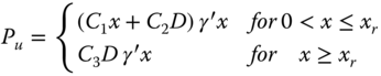
where:
- C1, C2, & C3
- Coefficient of lateral resistance
- (−)
- D
- Average pile diameter
- (m)

- Effective soil unit weight
- (kN m−3)
- xr
- Transition depth
- (m)
These coefficients are given in design charts as a function of the angle of internal friction as shown in (5.25). As well as characterising the ultimate lateral resistance, the initial modulus of subgrade reaction can also be obtained as shown in Figures 5.25 and 5.26.
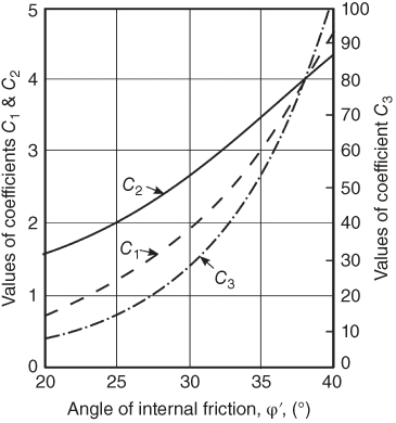
Figure 5.25 Lateral resistance coefficients as a function of internal angle of friction after American Petroleum Institute (1993).
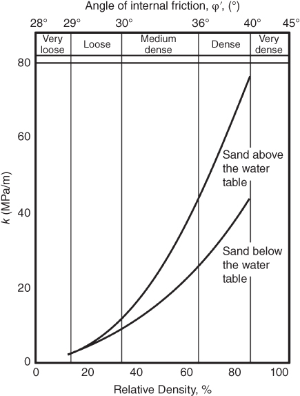
Figure 5.26 Initial modulus of subgrade reaction after Det Norske Veritas (2013) and API.
5.4.4.4 p‐y Curves for Clay
The p‐y curves for clay are generated based on the following parameters:
- p = Lateral soil resistance
- pu = Ultimate lateral soil resistance
- y = Lateral pile deflection
- yc = 2.5ε50.d
- ε50 = Characteristic strain at 50% of failure stress in undrained tests
- d = Pile diameter
The ultimate soil resistance is determined by Eq. (5.63):
where:
- Su
- =
- Undrained shear strength of the soil
- NP
- =
- Ultimate lateral soil resistance coefficient
It is often assumed that NP is 3 at mudline (X = 0) and increases to 9 at depths equal to or greater than Xr, which is given by Eq. (5.64). The depth calculated is often termed as transition depth.
where:

- =
- Effective unit weight of the soil
- J
- =
- A constant
For static loading, a p‐y curve can be defined using the coordinates given in Table 5.8.
Table 5.8 p‐y coordinates for a static loading.
| y (Deflection) | p (Soil reaction) |
| 0 | 0 |
| yc | 0.5 pu |
| 2 yc | 0.63 pu |
| 4 yc | 0.8 pu |
| 6 yc | 0.9 pu |
| 8 yc | pu |
| infinite | pu |
Figure 5.27 shows a typical p‐y curve for static loading based on Matlock (1970a,b). The curve is drawn by fitting a cubic parabola given by Eq. (5.65).
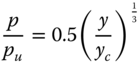
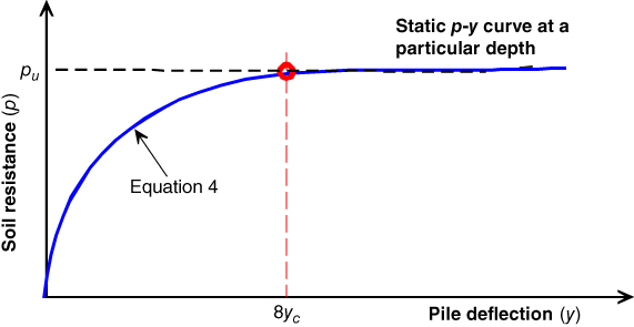
Figure 5.27 Static p‐y curves, Matlock (1970a,b).
The static p‐y curves are modified to express the deterioration due to cyclic loading.
Bhattacharya et al. (2006) recommended that for free‐headed piles, consideration should be given to incorporate the shear resistance across the base of the pile. This may be incorporated into a special p‐y curve at the tip of the pile, which has an ultimate resistance equal to the lateral shear of the soil across the full base of the pile. An appropriate displacement to mobilise the base shear can be idealised from elastic methods, or alternatively, from a full elasto‐plastic FEA. Monopiles or anchor piles for floating systems fall under such category.
5.4.4.5 Cyclic p‐y Curves for Soft Clay
The construction of cyclic p‐y curves for soft clay is empirical and was formulated to fit the observed pile load test at the Lake Austin and Sabine sites. The maximum cyclic resistance is limited to 0.72 pu. It is also assumed that complete loss in resistance occurs at the soil surface when deflections at that point reach 15 yc. The coordinates for cyclic p‐y curves are given in Table 5.9.
Table 5.9 p‐y coordinates for cyclic loading.
| y (Deflection) | p (Soil reaction) |
| 0 | 0 |
| yc | 0.5 pu |
| 3 yc | 0.72 pu |
| 15 yc | 0.72 pu (X/Xr) |
| Infinite | 0.72 pu (X/Xr) |
Figure 5.28 shows a typical cyclic p‐y curve. It must be remembered that the curve is constructed in order to fit the observed data. Matlock (1970a,b) cautions against three aspects of the curve that are primarily empirical:
- The position of the cyclic deterioration threshold, i.e. the coordinate (3 yc, 0.72 pu) along the pre‐plastic portion of the static p‐y curve
- The manner in which the residual resistance 0.72 pu(X/Xr) is adjusted with depth
- The value of the deflection at which the residual resistance occurs
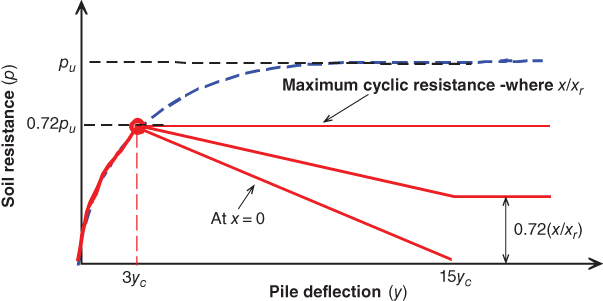
Figure 5.28 Cyclic p‐y curves for soft clays.
5.4.4.6 Modified Matlock Method
The p‐y curves developed by Reese et al. (1975) for stiff clay result from test piles loaded laterally in overconsolidated clay deposits. The clays at the test site ranged in strength from 96 kPa (surface) to 290 kPa at 3.6 m and had significant secondary structure (fissures, joints, and slickensides). ɛ50 values for stiff clays recommended in the paper range from 0.7% (shear strength 50–100 kPa) to 0.4% (shear strengths 200–400 kPa). Typical overconsolidated North Sea clays, however, do not usually show significant secondary structure, nor demonstrate the same trend in variation of ɛ50 with shear strength as recommended by Reese et al. (1975).
Matlock (1979) has suggested that for stiff clays, p‐y curves may be obtained using Matlock (1970a,b) with a modification applied above the transition depth Xr. It is in the zone above the transition depth that large deflections usually occur. Table 5.10 gives the coordinates to construct the modified p‐y curve. Essentially, the peak point in the cyclic p‐y curve for soft clays is omitted as shown in Figure 5.29. In this modified method, cyclic degradation starts at a deflection of yc where the soil reaction is equal to 0.5 pu. If soft clay cyclic curves had been used, cyclic degradation would have occurred at a deflection equal to 3 yc and the peak resistance would also have been approximately 50% higher.
Table 5.10 p‐y coordinates for cyclic loading for stiff clays (modified).
| y (Deflection) | p (Soil reaction) |
| 0 | 0 |
| yc | 0.5 pu |
| 15 yc | 0.72 pu (X/Xr) |
| Infinite | 0.72 pu (X/Xr) |
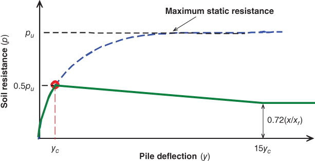
Figure 5.29 Modified Matlock cyclic p‐y curve, based on Bhattacharya et al. (2006). This p‐y curve is recommended in API and ISO code.
5.4.4.7 ASIDE: Note on the API Cyclic p‐y Curves
- In the API (2005) design approach, cyclic deterioration has been defined on the basis of an empirical fit to a limited pile load test database from Sabine and Lake Austin. Matlock cautions against the uncertainties regarding the position of the cyclic deterioration threshold and the distribution in which the residual resistance is adjusted with depth, and the value of the deflection at which the residual resistance occurs.
- Centrifuge tests carried out to verify the design of piles for the URSA (Mississippi Canyon Block 809) TLP Platform showed that, for cyclic behaviour of a single pile, large lateral displacements reduce Matlock's 0.72 factor by about 20%, i.e. a factor of 0.57 (Doyle et al. 2004). This provides some justification for the factor of 0.5 used as the peak resistance for cyclic p‐y curves in the modified Matlock approach.
- The data on the cyclic loading of soils indicate that soil degradation affects not only soil strength but also soil stiffness. However, the recommended cyclic p‐y curves do not reduce the initial pile response, i.e. pile stiffness when compared with the static p‐y curves. This is obviously at odds with observed cyclic behaviour of soils.
- ε50 is used to link the stiffness of the p‐y curves to the soil stiffness at the site. Therefore, this is an important design parameter and must be measured through advanced soil testing. Soils with a higher OCR are expected to have higher ε50 values.
- For free‐headed piles such as monopiles or anchor piles, where cyclic behaviour is very critical, it is therefore prudent to consider fundamental soil behaviour when deriving generalised cyclic p‐y data. Incorporation of degradation or increase in stiffness due to large cyclic loads must be linked in the p‐y curves.
5.4.4.8 Why API p‐y Curves Are Not Strictly Applicable
- The p‐y approach uses nonlinear springs and produces reliable results for the cases for which it was developed, i.e. small diameter piles and for few cycles of loading. For O&G applications, the main design requirement is ULS, i.e. avoiding plastic hinge in the pile. In other words, the ultimate strength of the soil i.e. nature of the p‐y curves at large strain level. On the other hand, for offshore wind monopile design, SLS and natural frequency is the main design criteria and therefore initial part of the p‐y curve is critical.
- The method is not validated yet for large‐diameter piles. Kallehave & Thilsted (2012) reported that using API p‐y curves underpredicts the foundation stiffness.
- API formulation doesn't consider the base resistance as well as shaft resistance, and this will have significant contribution for large‐diameter piles. The readers are referred to Shadlou and Bhattacharya (2016a) for analytical work considering the base resistance and shaft resistance.
5.4.4.9 References for p‐y Curves for Different Types of Soils
There are no code provisions or guidelines for soft rocks such as weak mudstone, sandstone, and carbonate materials. Different forms of p‐y curves have been proposed. Table 5.11 provides references for weak rocks along with liquefied soils and partially liquefied soils.
Table 5.11 Reference for p‐y curve construction for different types of soils.
| Type of soils | Reference for p‐y curves |
| Calcareous soils |
Wesselink et al. (1988) Williams et al. (1988) Dyson (1999) Dyson and Randolph (2000) |
| Weak rock | Reese et al. (1997) |
| Weak carbonate rock | Abbs (1983) |
| Weak calcareous claystone | Fragio et al. (1985) |
5.4.4.10 What Are the Requirements of p‐y Curves for Offshore Wind Turbines?
Ideally, the p‐y curves to be used for modelling pile–soil interaction should capture the two pile–soil interaction likely to be encountered in its lifetime:
- Effects of action of millions of cycles of loadings due to wind, wave, 1P, and 3P under operating conditions. It may be noted that the strains in the soil depend on the type of loading. As discussed in Chapter 4, sandy soils under very small strains will densify. On the other hand, sandy soils under moderate to large strains under undrained condition will partially or fully liquefy through the generation and accumulation of pore water pressure.
- Soil stiffness and strength will change under extreme loading conditions.
5.4.4.11 Scaling Methods for Construction of p‐y Curves
This section presents the modern way of developing p‐y curves from stress–strain curves of the corresponding soil. The scaling method for the construction of p‐y curves from stress–strain curves relies on the similarity between load‐deflection characteristics of the pile and mechanical behaviour of the deforming soil. This involves scaling of stress and strain into compatible soil reaction p and pile deflection y, respectively. Figures 5.30 and 5.24 show a schematic of the application and the values that are necessary are Ms and Ns. It is assumed that plane strain conditions are established around the pile at any depth. As a result, soil is expected to flow around the pile from front to back. Although such an assumption is acceptable at deeper depths, the same may not be valid at the surface level when wedge type failure is likely to occur, particularly at shallow depths. In accordance with the postulated collapse mechanism, the SSI problem reduces to a series of decoupled plane strain problems as schematically illustrated in Figure 5.30. The model considered here is therefore a disc having an outer radius of R, representing the soil, and a rigid disc with outer radius r0 that moves laterally in the deforming soil. The soil is further supposed to adhere perfectly to the pile. It should be emphasised that the conceptualised problem is analogous to the plane strain problem used in plasticity theory for the evaluation of the undrained lateral capacity of a cylinder moving through an infinite medium.
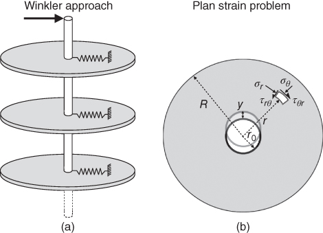
Figure 5.30 Schematic representation of the problem: (a) Winkler approach; (b) Plane strain model.
This method is similar to MSD method proposed by Osman and Bolton (2005). The key feature of the MSD approach is that a single stress and a single strain are chosen to represent the behaviour of the soil mass under any given loading conditions. The representative stress is related to the applied load, and the representative strain is related to the applied displacement. If a stress–strain relationship is known for the soil, then this can be converted to an equivalent load–displacement relationship for the chosen problem. Clearly, this approach cannot be expected to describe the detailed response with great accuracy, as a number of approximations are involved, most importantly a single stress value cannot represent the stress state of the entire soil mass and a single strain state cannot represent the strains in an entire soil mass.
Nevertheless, as demonstrated by Osman and Bolton, the approach lies within the tradition of robust engineering applications for two fundamental reasons: first, the MSD can provide a realistic estimate of load‐deformation behaviour, and second, it has a benefit that complex calculations are not required. The soil resistance p developed at a mobilised stress τmob is given by
in which Ns is a scaling factor for stress. The mobilised shear stress τmob can be related to an average mobilised engineering shear strain γs mob. This can be mathematically defined as the spatial average of the shear strain γs in the entire volume of the deforming medium. The engineering shear strain γs can be defined as the difference between the major and the minor principal strains:
The average shear strain mobilised in the deforming soil can be calculated from the spatial average of the shear strain in the whole volume of the deformation zone. This mobilised shear strain can be associated with the pile displacement as follows:
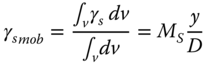
MS and NS are determined and presented in the work of Bouzid et al. (2013), Dash (2010), and Dash et al. (2017) and are summarised In (Table 5.12).
Table 5.12 Summary of MS and NS.
| Type of interface and soil model | MS | NS |
| Linear elastic soil with smooth interface | 3.15 | 11.23 |
| Linear elastic soil with rough interface | 2.59 | 17.89 |
| Rigid plastic with rough interface | 2.60 | 9.00 |
Similar scaling methods as that of Dash (2010), Bouzid et al. (2013) are also proposed by Zhang et al. (2016), Zhang and Andersen (2017), and Jeanjean (2017). Using the scaling method discussed of Bouzid et al. (2013), Lombardi et al. (2017), and Dash et al. (2017) presented p‐y curves for liquefied soils.
5.4.4.12 p‐y Curves for Partially Liquefied Soils
One of the first attempts to propose p‐y curves for liquefiable soils is provided by Liu and Dobry (1995). The method, illustrated in Figure 5.31, consists of applying to the conventional p‐y curve for nonliquefied sand a reduction factor mp also known as p‐multplier. mp is based on the excess pore water pressure ratio (![]() ) where u is the excess pore water pressure developed and
) where u is the excess pore water pressure developed and ![]() is the vertical effective stress. ru of 1 implies full liquefaction and mp is 0 and ru of 0 would imply no liquefaction and mp is 1. Linear interpolation is allowed and this model is reasonable for partially liquefied soils. This model will predict a flat curve, i.e. no springs for fully liquefied soils. While this is a valid assumption for small amplitude vibration, it is unrealistic for large amplitude. The next section shows a p‐y curve for fully liquefied soils developed based on the scaling method.
is the vertical effective stress. ru of 1 implies full liquefaction and mp is 0 and ru of 0 would imply no liquefaction and mp is 1. Linear interpolation is allowed and this model is reasonable for partially liquefied soils. This model will predict a flat curve, i.e. no springs for fully liquefied soils. While this is a valid assumption for small amplitude vibration, it is unrealistic for large amplitude. The next section shows a p‐y curve for fully liquefied soils developed based on the scaling method.
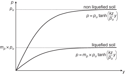
Figure 5.31 Construction of p‐y curves for liquefiable soils according to p‐multiplier approach.
5.4.4.13 p‐y Curves for Liquefied Soils Based on the Scaling Method
Figure 5.32 presents p‐y curves for liquefied soils based on the work on Lombardi et al. (2017) and Dash et al. (2017). The method is schematically shown in Figure 5.32. For this method, a multistage cyclic triaxial test is required. First, the soil is cyclically loaded to full liquefaction and when the soil is fully liquefied, monotonic load is applied and the stress–strain curve is obtained. Through the advanced testing of wide range of sandy soils, Rouholamin et al. (2016) showed that stress–strain curve for liquefied soil looks like Figure 5.32a and the important parameter is the take‐off strain (γto). Take‐off strain is the strain at which the soil grains of the initially liquefied soil start to lock and resistance is developed. Once the simplified stress–strain model of liquefied soil is formulated, the corresponding p‐y curve parameters are calculated by using scaling factors, Ms and Ns. Figure 5.32 schematically represents the process involved in transforming stress–strain model to the p‐y curve of liquefied soil. The readers are referred to the paper by Dash et al. (2017) for further details and an example application.
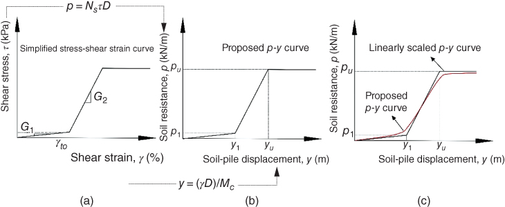
Figure 5.32 Use of scaling approach for derivation of p‐y curves from stress–strain response of liquefied soils.
5.4.5 Advanced Methods of Analysis
For the current application, advanced method of analysis represents finite element, discrete element, or finite difference methods. Discussion of these methods is beyond the scope of this book. Figure 5.33 shows a model of the whole problem. The advantage of this method is that complex soil behaviour can be incorporated. For example, to account for long‐term performance prediction, it is necessary to employ a suitable constitutive model, capable of reproducing realistic soil behaviour when subjected to cyclic/dynamic loading conditions. Simple elastoplastic models are usually based on one yield surface without hardening (e.g. the Mohr coulomb model), with isotropic hardening (e.g. the Cam‐Clay model), or on two yield surfaces (isotropic loading and deviatoric loading), e.g. Lade's. They are ideal and efficient on simulating the soil behaviour under monotonic conditions, but not suitable for model cyclic loading. Essentially, in such models, plastic deformations start to appear for a certain magnitude of loading, usually higher than the amplitude of the cycles, and hence, the simulated soil behaviour remains elastic under that limit, which is against experimental evidences, particularly for granular soils Cambou and Hicher (2008). Figure 5.34 shows the different phenomenon that can take place in soil during cyclic loading.
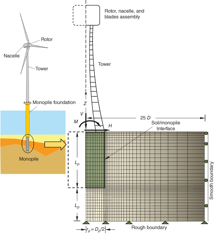
Figure 5.33 Finite element of a monopile and surrounding elastic medium.
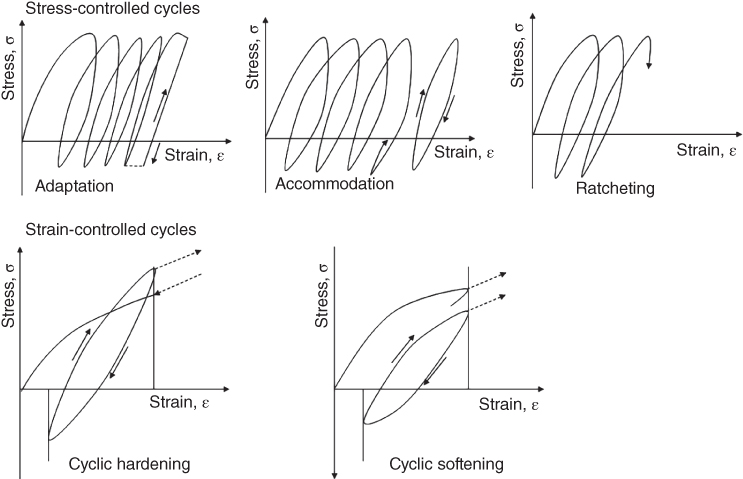
Figure 5.34 Different cyclic behaviours.
Plastic phenomenon for cyclic loading can either be based on constant stress amplitude (so called stress controlled) or constant strain amplitude (strain controlled). The phenomenon called adaptation refers to less dissipation of energy in each cycle of loading as the number of cycles increases, until convergence to nondissipative elastic cycles. On the other hand, accommodation refers to change of the dissipation of energy from the beginning with an irreversible cumulative deformation and evolves towards a stabilised cycle. This is experienced in laboratory experiments for drained samples. Ratcheting is an irreversible strain accumulation, which keeps the same shape as that of the beginning.
Constant strain amplitude cyclic loading phenomenon results in the cyclic hardening or softening. Cyclic hardening occurs when there is an increase in the cyclic stress amplitude with an increase in the number of cycles, e.g. densification during testing of drained soil. On the contrary, cyclic softening occurs when there is a reduction in the cyclic stress amplitude as the number of cycles increases, e.g. an increase in pore pressure during the testing of undrained soil samples (decrease in the effective stress).
A kinematic hardening law may be employed by coupling the elastic moduli and the hardening parameter. Kinematic hardening can be used to model plastic ratcheting, which is the build‐up of plastic strain during cyclic loading, as previously explained. Other hardening behaviours include changes in the shape of the yield surface in which the hardening rule affects only a local region of the yield surface, and softening behaviour in which the yield stress decreases with plastic loading. The kinematic hardening model involves only one plastic mechanism with a smooth yield surface. For nonlinear modelling, the material behaviour is characterised by an initial elastic response, followed by plastic deformation and unloading from the plastic state. The plasticity is a result of the microscopic nature of the material particles and includes shear loading that causes particles to move past one another, changes in void or fluid content that result in volumetric plasticity, and exceeding the cohesive forces between the particles or aggregates. The material is defined by model materials subject to loading beyond their elastic limit. Figure 5.35 shows a PLAXIS model for suction caisson type foundations.
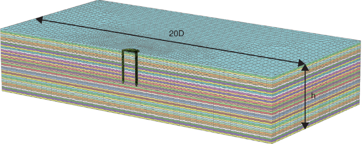
Figure 5.35 Soil model used to simulate parabolic stiffness variation in PLAXIS 3D.
The readers are referred to Lopez Querol et al. (2017) for advanced numerical model analysis of monopile.
5.4.5.1 Obtaining KL, KR, and KLR from Finite Element Results
This section shows a method to compute the three stiffness terms (KL, KLR, and KR) from FEA. Mathematically, two FEA analyses are required and there are pile‐head moment‐rotation (M‐θ) and pile‐head horizontal load‐deflection (H‐δ). Considering the full range of the curve, i.e. until failure, pile‐head load‐deflection and pile‐head moment‐rotation curves are nonlinear, depending on the soil type. However, the initial linear range of the curves must be used to estimate pile‐head rotation and deflection based on Eq. (5.69).
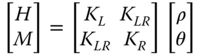
Eq. ( 5.69) can be rewritten as Eq. (5.70) through matrix operation where I (flexibility matrix) is a 2 × 2 matrix given by Eq. (5.71):
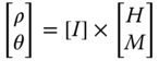
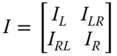
To obtain the stiffness components, run a numerical model for a lateral load (say H = H1) with zero moment (M = 0) and obtain values of deflection and rotation (ρ1 and θ1). The results can be expressed through Eqs. (5.72)–(5.73).
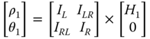
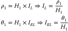
Similarly, another numerical analysis can be done for a defined moment (M = M1) and zero lateral load (H = 0) and the results are shown in Eqs. (5.74)–(5.75).
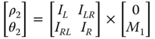
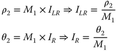
From the above analysis (Eqs. ( 5.72)−( 5.75)), terms for the matrix (Eq. ( 5.71)) can be obtained. Eq. ( 5.70) can be rewritten as Eq. (5.76) through the matrix operation.
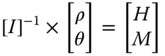
Comparing Eqs. ( 5.69) and ( 5.76), one can easily see the relation between the stiffness matrix and the inverse of flexibility matrix (I) given by Eq. (5.77). Equation (5.78) is a matrix operation that can be carried out easily to obtain KL, KR, and KLR.
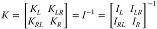
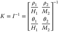
It is important to note that the above methodology is only applicable in the linear range, and therefore it is advisable to obtain a load‐deflection and moment‐rotation curve to check the range of linearity even if a nonlinear soil model is used. If the analysis is used beyond the linear range, deflections and rotations will be underestimated. An example application is shown in Chapter 6.
The above method can also be used with the standard method of analysis. Essentially, one needs load‐deflection and a moment‐rotation curves.
5.5 Long‐Term Performance Prediction for Monopile Foundations
Monopiles are commonly used foundations for these turbines in water depths of less than about 30 m. Figure 5.36 shows a schematic diagram of a monopile‐supported wind turbine with the main cyclic and dynamic loads acting on the turbine. As discussed in Chapter 2, wind and wave provides the largest overturning moment.
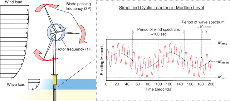
Figure 5.36 Loads acting on a typical OWT foundation and typical mudline moment.
Typically, in shallow to medium deep waters, the wind thrust loading at the hub will produce the highest cyclic overturning moment at the mudline. However, the frequency of this loading is extremely low and is in the order of magnitude of 100 seconds as shown in Figure 5.36. For further details the readers are referred to Chapter 2. Typical period of wind turbine structures being in the range of about 3 to 5 seconds, and therefore no resonance of structure due to wind turbulence is expected. Therefore, this is cyclic soil–structure interaction (CSSI) rather than DSSI. On the other hand, the wave loading will also apply overturning moment at the mudline and the magnitude depends on water depth, significant wave height, and peak wave period. Typical wave period will be in the order of 10 seconds (for North Sea) and will therefore have DSSI.
A calculation procedure developed in Arany et al. (2017) and related examples are presented in Chapters 2 and 6, whereby overturning moments can be estimated for various load cases on wind and wave. The output of such a calculation will be relative wind and the wave loads given by Mmax, Mmin, and Mmean as shown in Figure 5.36. It is assumed in the analysis that the wind and wave are perfectly aligned, which is a fair assumption for deeper water further offshore projects (i.e. fetch distance is high). Analysis carried out in Chapter 2 showed that the loads from 1P and 3P are orders of magnitude lower than wind and wave, but they will have the highest dynamic amplifications. The effect of dynamic amplifications due to 1P and 3P will be small amplitude vibrations.
Furthermore, there are added soil–structure interactions due to many cycles of loading and the wind–wave misalignments. Typical estimates will suggest that OWT foundations are subjected to 10–100 million load cycles of varying amplitudes over their lifetime (25–30 years). The load cycle amplitudes will be random/irregular and have broadband frequencies ranging several orders of magnitudes from about 0.001 to 1 Hz. Based on the discussion above, the soil–structure interaction can be simplified into two superimposed cases and is shown in Figure 5.37.
- Cyclic overturning moments (typical frequency of 0.01 Hz) due to lateral loading of the wind acting at the hub together with that of the wave. This will be similar to a fatigue‐type problem for the soil and may lead to strain accumulation in the soil giving rise to progressive tilting. Due to wind–wave load misalignment, the problem can also be multidirectional.
- Wave loading, on the other hand, will be dynamic to different degree (mild/moderately/high), i.e. mildly dynamic or moderately dynamic or highly dynamic. This depends on the location of the wind farm and more specifically wave spectrum and the target frequency of the turbine. An 8 MW turbine supported of monopiles having 0.22 Hz as the first eigen frequency located in the North Sea (having 0.1 Hz predominant wave frequency) will be moderately dynamic. The same turbine in the China Sea having 5 seconds predominant period will be highly dynamic.
- Due to the proximity of the frequencies of 1P and 3P to the natural frequency of the structure, resonance in the wind turbine system is expected. Field evidence also supports this; see Hu et al. (2014) with reference German wind farm projects. Studies presented in Chapter 2 show that these are orders of magnitude lower than that caused by the wind and the wave. This resonant dynamic bending moment will cause cyclic strain in the pile in the fore–aft direction, and this strain will be transferred to the neighbouring soil. This resonant type mechanism will involve compaction of the soil in front of and behind the pile (in the fore–aft direction). This is shown by a SDOF oscillator in Figure 5.37.
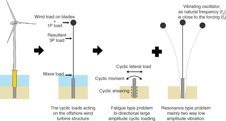
Figure 5.37 Loads acting on a monopile‐supported wind turbine.
5.5.1 Estimation of Soil Strain around the Foundation
In the whole turbine structure, i.e. RNA‐Tower‐Transition Piece‐Monopile‐Soil, the element that is most likely to change with the operation is the soil. Other materials such as steel may change due to fatigue‐type loading, but the change is miniscule compared to the soil. In routine engineering practice, SSI can be incorporated through the estimation of strain levels in the deformed/mobilised zone by considering the soil behaviour at that strain level. A method is developed based on the above and explained below:
Deformation of the pile under the action of the loading as described in Section 5.5 and Figure 5.37 will lead to three‐dimensional soil–pile interaction, as shown schematically in Figure 5.38. Simplistically, there would be two main interactions:
- Due to pile bending (which is cyclic in nature) and the bending strain in the pile, strain in the soil will transfer through contact friction, which will be cyclic in nature.
- Due to lateral deflection of the pile, strain will develop in the soil around the pile.
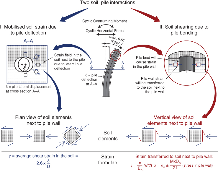
Figure 5.38 Two types of soil‐pile interaction on a monopile‐supported wind turbine. A simple model is proposed in Nikitas et al. (2017).
Figure 5.38 also shows a simple methodology to estimate the levels of strains in a soil for the two types of interactions, and is given by Eqs. 5.79 and 5.80.
The average strain in the soil at any section in a pile due to deflection can be estimated using Bouzid et al. (2013):

where δ is the pile deflection at that section (for example A‐A in Figure 5.38) and DP is the pile diameter. This is also explained in some details in Figure 5.39 and the readers are referred to Lombardi et al. (2013) for further details.
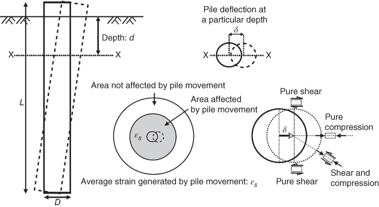
Figure 5.39 Average strain in the soil around a pile.
On the other hand, the shear strain in the soil next to the pile due to pile bending can be estimated using Eq. ( 5.80).
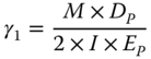
where M is the bending moment in the pile, I is the second moment of area of pile and EP is the Young's modulus of the pile material. It must be mentioned that Eq. ( 5.80) assumes that 100% of the strain is transmitted to the soil, which is a conservative assumption and calls for further study. In practice, this will be limited to the mobilisable friction between the pile and the soil. The above methodology is used to estimate the strain levels in the soil for 15 wind turbines.
This strain level can then be used to carry out element tests of the soil and obtain parameters. If the strain is high for a clayey soil, residual strength may be taken for calculations. If the strain is medium, appropriate strength and stiffness degradation curves may be used. The readers are referred to Chapter 4 for further understanding of soil behaviour for a wide range of strains.
5.5.2 Numerical Example of Strains in the Soil around the Pile for 15 Wind Turbines
In this section, 15 wind turbines from 12 wind farms (Figure 5.40) are analysed to show the application of the methodology. For all 15 wind turbines, the loads are calculated using the methodology developed in Chapter 2 , and an example is shown in Chapter 6. The input parameters for the load calculation are shown in Tables 5.13−5.15. For the case studies, the strains in the soil are estimated based on the methods discussed in the earlier section and depicted in Figure 5.38. They are:
- The pile wall strain is assumed to be have been transferred fully to the soil in contact with the pile wall. This will typically extend to few soil grain diameters. Apart from these small amplitude strains (due to wind and wave), along the length of the pile small‐magnitude vibrations (resonance due to the proximity of 1P and 3P loading) will cause the soil to compact. Equation ( 5.80) can be used for such strain calculations, and the bending moment along the pile is required for such estimate. The soil strain can be computed for different load conditions. Figures 5.41 and 5.42 plot the strain for normal working condition and extreme load condition. It may be noted that the strain in the soil due to resonance is neglected as the moments due to 1P and 3P are orders of magnitude lower than wind and wave moments.
- Large amplitude cyclic loads (wind + wave) cause deflections along the pile length and shear strains are developed in the soil surrounding the pile. These strains, if high enough, can cause degradation in soil stiffness. These shear strains may be estimated for normal working condition using the formulas given in Eq. ( 5.79). Figures 5.43 and 5.44 provide strain distribution in the soil along the length of the pile for two conditions.
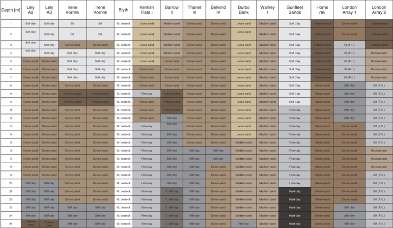

Figure 5.40 Ground profile for 12 wind farm sites.
Table 5.13 Soil parameters assumed for typical sandy soils in p‐y analysis (Beam on Nonlinear Winkler Foundation approach).
| Sand p‐y parameters | Very loose | Loose | Medium | Dense | Very dense |
| Friction angle (φ′) | 28 | 30 | 33 | 38 | 40 |
| Effective unit weight (γ′ [kN m−3]) | 6 | 7 | 8 | 9 | 10 |
| Relative density (Rd) | 15 | 20 | 40 | 60 | 80 |
| Initial stiffness gradient (k) (kPa m−1) | 3 000 | 8 000 | 16 000 | 30 000 | 40 000 |
Table 5.14 Soil parameters assumed for typical clayey soils in p‐y analysis.
| Clay p‐y parameters | Soft | Firm | Stiff | Very stiff | Hard |
| Undrained shear strength (cu) | 25 | 50 | 100 | 200 | 400 |
| J parameter (−) | 0.25 | 0.25 | 0.25 | 0.25 | 0.25 |
| Strain, 50% failure stress (ε50[−]) | 0.007 | 0.006 | 0.005 | 0.004 | 0.003 |
| Effective unit weight (γ′ [kN m−3]) | 7 | 8 | 9 | 10 | 12 |
| Young's modulus (ES [MPa]) | 1.25 | 2.5 | 5 | 10 | 20 |
Table 5.15 Parameters used for the calculations.
| Parameter | Symbol (unit) | Lely A2 | Lely A3 | Irene Vorrink | Irene Vorrink | Blyth | Kentish I | Barrow II | Thanet III | Belwind IV | Burbo Bank | Walney I | Gunfleet Sands | Horns Rev | London Array 1 | London Array 2 |
| Reference turbulence intensity | I15 (%) | 18.0 | 18.0 | 18.0 | 18.0 | 180 | 18.0 | 18.0 | 18.0 | 18.0 | 18.0 | 18.0 | 18.0 | 18.0 | 18.0 | 18.0 |
| Rated wind speed | UR (m s−1) | 14.0 | 14.0 | 14.0 | 14.0 | 17.0 | 15.0 | 15.0 | 15.0 | 15.0 | 14.0 | 14.0 | 14.0 | 16.0 | 12.5 | 12.5 |
| Rotor diameter | D (m) | 43.0 | 43.0 | 43.0 | 43.0 | 66.0 | 90.0 | 90.0 | 90.0 | 90.0 | 107.0 | 107.0 | 107.0 | 80.0 | 120.0 | 120.0 |
| Hub height above mean sea level | zhub (m) | 41.5 | 41.5 | 48.8 | 48.8 | 67.0 | 70.0 | 75.0 | 70.0 | 72.0 | 83.5 | 83.5 | 75.5 | 70.0 | 87.0 | 87.0 |
| Mean water depth | S (m) | 12.1 | 7.1 | 5.2 | 6.0 | 7.8 | 8.0 | 18.0 | 27.0 | 20.0 | 8.0 | 21.5 | 15 | 14.0 | 25.0 | 10.0 |
| Maximum wave height before breaking | Hbreak (m) | 9.4 | 5.5 | 4.1 | 4.7 | 8.6 | 6.2 | 14.0 | 21.1 | 15.6 | 6.2 | 16.8 | 11.7 | 10.9 | 19.5 | 7.8 |
| Breaking wave time period | Tbreak (s) | 10.9 | 8.3 | 7.1 | 7.7 | 10.4 | 8.9 | 13.3 | 16.3 | 14.0 | 8.9 | 14.5 | 12.1 | 11.7 | 15.6 | 9.9 |
| 50‐yr maximum wave height | HE50 (m) | 9.4 | 5.5 | 4.1 | 4.7 | 8.6 | 6.2 | 14.0 | 21.1 | 15.6 | 6.2 | 16.8 | 11.7 | 10.9 | 19.5 | 7.8 |
| 50‐yr maximum wave period | TE50 (s) | 10.9 | 8.3 | 7.1 | 7.7 | 10.4 | 8.9 | 13.3 | 16.3 | 14.0 | 8.9 | 14.5 | 12.1 | 11.7 | 15.6 | 9.9 |
| 50‐yr significant wave height | HS50 (m) | 5.1 | 3.0 | 2.2 | 2.5 | 4.6 | 3.4 | 7.5 | 11.3 | 8.4 | 3.4 | 9.0 | 6.3 | 5.9 | 10.5 | 4.2 |
| 50‐yr peak wave period | TS50 (s) | 8.0 | 6.1 | 5.2 | 5.6 | 7.6 | 6.5 | 9.7 | 11.9 | 10.3 | 6.5 | 10.6 | 8.9 | 8.6 | 11.5 | 7.3 |
| 1‐yr maximum wave height | HE1 (m) | 7.6 | 4.5 | 3.3 | 3.8 | 6.9 | 5.0 | 11.3 | 16.9 | 12.5 | 5.0 | 13.5 | 9.4 | 8.8 | 15.7 | 6.3 |
| 1‐yr maximum wave period | TE1 (s) | 9.8 | 7.5 | 6.4 | 6.9 | 9.3 | 7.9 | 11.9 | 14.6 | 12.6 | 7.9 | 13.0 | 10.9 | 10.5 | 14.0 | 8.9 |
| 1‐yr significant wave height | HS1 (m) | 4.1 | 2.4 | 1.7 | 2.0 | 3.7 | 2.7 | 6.0 | 9.1 | 6.7 | 2.7 | 7.2 | 5.0 | 4.7 | 8.4 | 3.4 |
| 1‐yr significant wave period | TS1 (s) | 7.1 | 5.5 | 4.7 | 5.0 | 6.8 | 5.8 | 8.7 | 10.7 | 9.2 | 5.8 | 9.5 | 8.0 | 7.7 | 10.3 | 6.5 |
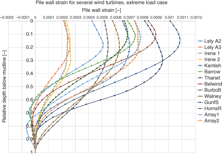
Figure 5.41 Pile wall strain along the length of the pile (extreme load case).
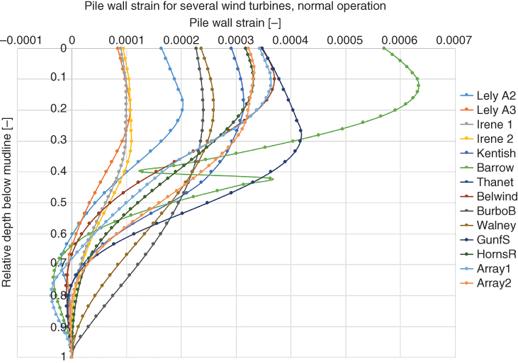
Figure 5.42 Pile wall strain (normal operating condition).
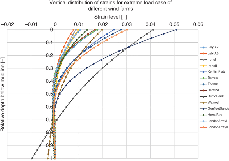
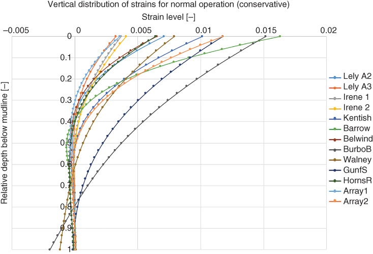
Figure 5.44 Soil strain along the length of the pile (normal operating condition).
There are therefore two opposing effects. The cyclic deflections may cause degradation in soil stiffness and may result in accumulated tilt as well as possible change in natural frequency. On the other hand, the small strains very close to the pile may cause compaction and may have a healing effect.
From the element test of a soil, it is known that strains below a certain limiting value do not cause degradation of the soil stiffness and do not change the behaviour significantly. Therefore, by estimating the strain magnitudes and comparing with results of element testing, one can determine whether degradation and thus accumulated tilt and changing natural frequency is to be expected.
5.6 Estimating the Number of Cycles of Loading over the Lifetime
One of the most challenging tasks in the analysis of the long‐term behaviour of offshore wind turbines is the estimation of the number of cycles of loading of different magnitudes that will have an impact on the performance. This information is necessary to predict the fatigue life of the monopile, as well as to predict the accumulated mudline deformations throughout the lifetime of the structure. To properly estimate the number of cycles at different load levels, a series of time domain simulations are necessary to statistically represent all operational states of the turbine in different environmental conditions. Rainflow counting (Matsuishi and Endo 1968) can be used to count the number of cycles from these time domain simulations. There are many other cycle counting methods available, such as peak counting, level‐crossing counting, simple‐range counting, range‐pair counting, and reservoir counting. These methods, as well as rainflow counting, are defined in (ASTM 2005). Researchers have provided simple empirical formulae for estimating the accumulated rotation, and the simple linear damage accumulation rule (Miner 1945) can be used to assess the fatigue life. However, without detailed data about the wind turbine and sophisticated simulation tools, it is challenging to estimate the number of load cycles.
Soil behaviour is a function of strain level. Under large strains, soil behaves highly nonlinearly. Loose to medium dense sands may progressively build pore water pressure and liquefy. At certain threshold strains, some soils (clayey soil) may degrade while others may compact. With episodes of low strain level and under the action of tens of millions of load cycles, some soils may increase their stiffness. Therefore, to predict the long‐term performance, one needs to know the corresponding wave height and wave period for maximum wave load calculation that will impose the largest moment in the foundation and the corresponding strain level. It is also necessary to estimate the number of cycles of loading that would influence the soil behaviour. Therefore, one needs to estimate the number of cycles of loading in a 3‐hour sea state by calculating the worst‐case scenario time period of wave loading. A method to predict the number of wave cycles is shown below in Section 5.6.1. The wind load cycles are typically at a much lower frequency than waves, but conservatively it is assumed that the wind and wave act at the same frequency, i.e. the frequency of the wave loading.
5.6.1 Calculation of the Number of Wave Cycles
In this step, a simplified estimation of the extreme wave height and the corresponding wave period for a given site is explained which involves the following sub‐steps:
- Obtain the relevant significant wave height HS from a reliable source.
- Calculate the corresponding range of wave periods, TS.
- Calculate the number of waves in a 3‐hour period, N.
- Calculate the maximum wave height, Hm.
- Calculate the range of wave periods corresponding to the maximum wave height, Tm.
The sub‐steps are now described in detail.
5.6.1.1 Sub‐step 1. Obtain 50‐Year Significant Wave Height
In absence of site‐measured data, one can use data from offshore drilling stations or other sea state monitoring reports. For the United Kingdom, the document ‘Wave mapping in UK waters’, periodically prepared for the Health and Safety Executive, can be used (Williams 2008). In this document one can find nearby O&G stations or meteorological buoys and estimate the 50‐year significant wave height at the wind farm site from that.
5.6.1.2 Sub‐step 2. Calculate the Corresponding Range of Wave Periods
The range of wave periods for a given wave height can be estimated following DNV‐OS‐J101 (DNV 2014), and the following formula may be used:
Typically, the most severe wave loads (following Morrison's equation or the McCamy‐Fuchs diffraction solution) are produced by the lowest wave period, and the dynamic amplification is also highest since the frequency is closest to the natural frequency of the structure. Therefore, the peak wave period is taken as
5.6.1.3 Sub‐step 3. Calculate the Number of Waves in a Three‐Hour Period
Typically, significant wave heights are given for a 3‐hour period. In other words, this means that the significant wave height is calculated as the mean of the highest 1/3 of all waves. Therefore, many different wave heights occur within this 3‐hour period, and the highest occurring wave height is called the maximum wave height Hm. To find this, one needs to know the number of waves in the 3‐hour period, because the more waves there are, the higher the chance of higher waves occurring.
5.6.1.4 Sub‐step 4. Calculate the Ratio of the Maximum Wave Height to the Significant Wave Height
The DNV code suggests taking the mode of the distribution of the highest wave heights, and thus:
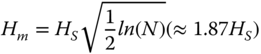
The maximum wave height may be taken conservatively as Hm = 2HS. Please note that the water depth S may limit the maximum wave height. Typically, it is assumed that the breaking limit of waves (i.e. maximum possible wave height) in water depth S is ![]() . However, if the seabed has a slope, the wave may be higher than this limit, as was reported at the exposed site at Blyth (Camp et al. 2004). Therefore caution should be exercised when using this limit wave height.
. However, if the seabed has a slope, the wave may be higher than this limit, as was reported at the exposed site at Blyth (Camp et al. 2004). Therefore caution should be exercised when using this limit wave height.
5.6.1.5 Sub‐step 5. Calculate the Range of Wave Periods Corresponding to the Maximum Wave Height
The same formulae can be used as in Sub‐step 2.
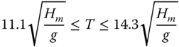
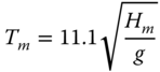
The wave height and wave period combination of Hm, Tm can be used for maximum wave load calculation, incorporating dynamic amplification.
5.7 Methodologies for Long‐Term Rotation Estimation
It may be noted that this is an area of active research. To fulfil the SLS requirements, the long‐term behaviour of monopile foundations needs to be analysed according to DNV (2014). The main concern is the accumulated rotation Δθ and deflection Δρ (or equivalently the strain accumulation) at the mudline level. Even though the analysis is required by design standards, there is no consensus on an accepted methodology to carry out this analysis. Several approaches have been proposed based on extremely simple load scenarios, such as a cyclic excitation, which can be described by a mean load Mmean, a cyclic load magnitude Mamp = Mmax − Mmin, and number of cycles,N. The actual load acting on an OWT foundation, however, is extremely complicated and it is important to highlight the complexity:
- The loading is not cyclic but in some case it may be dynamic. Loads applied are in a very wide frequency band ranging through the orders of magnitudes between 0.001–10 Hz, which includes the first few structural natural frequencies and blade natural frequencies. It is therefore difficult to estimate the numbers of load cycles. On the other hand, the frequency may be important in the determination of accumulated tilt. Even though it seems unlikely, it is not yet clear whether any significant excess pore pressures can occur and cause dynamic effects.
- Some of the available methods were developed for very low number of cycles. Long and Vanneste (1994) points out that implicit numerical simulations typically allow for simulation of less than 50 cycles due to the accumulation of numerical errors. Furthermore, most reported tests they analysed were also carried out for 50 cycles or less and only one test had 500 cycles. The authors suggest caution when predicting the effects of very high numbers of load cycles. The numerical investigations and laboratory tests carried out by Achmus et al. (2009) and Kuo et al. (2012) go up to 10 000 cycles, and tests by Leblanc et al. (2010) have been carried out for up to 65 000 cycles. However, these are still orders of magnitudes below the expected number of load cycles of an OWT. Cuéllar (2011) has run four tests with different load scenarios for a remarkable five million cycles and identified qualitative behaviour of deformation accumulation for a high number of cycles.
- The magnitude of dynamic loading also ranges from small to extreme loads, with load cycles ranging from a few to a few hundred cycles of extreme loads, and from millions to hundreds of millions of cycles of low‐amplitude vibrations. In different states of the wind turbine different load magnitudes are expected.
- The loading is not either one‐way or two‐way, but the whole range of load regimes are present at different times throughout the lifetime of the turbine. There is also disagreement in terms of whether one‐way or two‐way loading is more detrimental. Long and Vanneste (1994) suggest that one‐way loading is the critical load scenario and two‐way loading causes less accumulated strain. Achmus et al. (2009) and Kuo et al. (2012) also focus on one‐way loading in their analysis. However, Leblanc et al. (2010) found that the most critical scenario is two‐way loading with Mmin/Mmax = − 0.5.
- The loading is not unidirectional, loads appear both in the along‐wind (x) and cross‐wind (y) directions during the operational life of the turbine, and cyclic vertical (z) loads are also present. Wind and waves are also not always collinear, causing multidirectional loading on the foundation.
- The nacelle always turns into the wind, which means that the along‐wind (x) and cross‐wind (y) directions are not fixed in a global frame of reference but are turning as the yaw angle of the rotor changes. This means that the foundation is loaded both with along‐wind and cross‐wind loads throughout the lifetime of the turbine in all directions.
In pile design for offshore wind turbines, the p‐y method is typically employed. Long and Vanneste (1994) give a good account of the research efforts into the analysis of piles under cyclic lateral loading by modified cyclic p‐y curves. Improved p‐y curves for cyclic lateral load were developed by Reese et al. (1974), O'Neill and Murchinson (1983), Little and Briaud (1988). More fundamental theoretical approaches have been attempted by Swane and Poulos (1982) as well as Matlock et al. (1978). As Long and Vanneste (1994) points out, these methods require parameters that are typically not available from site investigation.
The simplified approach of accumulated strain is often used in literature, which is equivalent to reduction of soil stiffness. The coefficient of subgrade reaction nh can be reduced in order to account for the effects of cyclic loading. Such an approach was used by Prakash (1962), Davisson (1970), and Davisson and Salley (1970). Broms (1964) pointed out that the reduction of nh depends on the density of the cohesionless soil. These studies suggest reducing nh by a fixed percentage if a certain number of load cycles (∼50) are expected (30% in Davisson (1970), 75% and 50% for dense and loose sand in Broms (1964)).
Logarithmic expressions for permanent strains of monopiles have also been proposed by Hettler (1981), Lin and Liao (1999), Verdure et al. (2003), Achmus et al. (2009), and Li et al. (2010). Power law expressions have been proposed for monopiles by Little and Briaud (1988), Long and Vanneste (1994), Leblanc et al. (2010), Klinkvort et al. (2010), and for caissons by Zhu et al. (2012) and Cox et al. (2014). Cuéllar (2011a,b) proposes a method by which three different curves are used to approximate the long‐term accumulation.
Some important contributions are listed below.
5.7.1 Simple Power Law Expression Proposed by Little and Briaud (1988)
Little and Briaud (1988) proposed the simple power law expression for strain accumulation:
where εN is the strain after N cycles, ε1 is the strain at the first load cycle and m is a constant that expresses dependence on soil and pile parameters, installation methods, and loading characteristics. Achmus et al. (2009) uses m = 0.136 for typical monopiles.
5.7.2 Degradation Calculation Method Proposed by Long and Vanneste (1994)
Long and Vanneste (1994) provide a simple approach for calculating the degradation of the coefficient of subgrade reaction determined from the analysis of 34 different load test scenarios. The degradation is expressed as
where nhN is the coefficient after N cycles of loading, nh1 is the coefficient at the first cycle, and t is the degradation parameter, which can be calculated according to
Fr, Fi, Fd are parameters to take into account the cyclic load ratio, pile installation method and soil density, respectively. For a driven pile (Fi = 1.0) in medium sand (Fr = 1.0) under one‐way loading (Fr = 1.0), the degradation parameter is t = 0.17.
Long and Vanneste (1994) emphasise that the load tests that serve as the basis of their analysis were mostly carried out for less than 50 load cycles, with only one test going up to 500. They suggest caution when applying these results for more than 50 load cycles, making the method hard to implement for OWT foundations where load cycles in the orders of magnitudes of 102 − 108 are expected. Furthermore, Long and Vanneste (1994) point out that the most important factor is the cyclic load ratio Mmin/Mmax , however, in their formulation the reduction in the coefficient of subgrade reaction is not explicitly dependent of the cyclic load magnitude.
5.7.3 Logarithmic Method Proposed by Lin and Liao (1999)
Lin and Liao (1999) provide a logarithmic expression for strain accumulation:
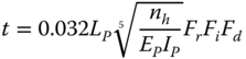
LP is the embedded length of the pile, Fr, Fi, Fd are parameters to take into account the cyclic load ratio, pile installation method and soil density, respectively. In the basic case of a driven pile in dense sand in one‐way loading, t = 0.032LP/T where ![]() is the pile/soil relative stiffness ratio, with nh being the coefficient of subgrade reaction.
is the pile/soil relative stiffness ratio, with nh being the coefficient of subgrade reaction.
Lin and Liao (1999) also provide a methodology to combine loads at different load levels into a single load case for the calculation of accumulated strain. This is achieved by converting all load cycles to a single load level by the method of equivalent accumulated strains. If there are two loads, say a and b, with ta and tb as degradation parameters and Na and Nb as numbers of load cycles, respectively, then
where ![]() is the equivalent load cycle number of load a in terms of the degradation parameter tb expressed as
is the equivalent load cycle number of load a in terms of the degradation parameter tb expressed as
5.7.4 Stiffness Degradation Method Proposed by Achmus et al. (2009)
Achmus et al. (2009) and Kuo et al. (2012) carried out laboratory tests and developed a numerical modelling procedure for analysing the long‐term mudline deformations of rigid monopiles. According to their stiffness degradation method, the increase in plastic strain due to cyclic loading can be interpreted as a decrease in the soil's Young's modulus ES:

where εpN = 1 is the plastic strain at the first load cycle, εpN is the plastic strain at the Nth cycle, and similarly for the elastic modulus. The following semi‐empirical approach for strain accumulation is used:
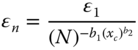
where:
Basic design charts for preliminary design are presented in Achmus et al. (2009) for the pile‐head deflection; the rotation is only slightly touched on in the paper.
5.7.5 Accumulated Rotation Method Proposed by Leblanc et al. (2010)
Leblanc et al. (2010) carried out tests for rigid piles in sand to assess the long‐term behaviour in terms of accumulated rotation at the mudline. Their tests were carried out using two main parameters:

which describes the magnitude of loading with respect to the static moment resisting capacity of the pile MR. The values are between 0 and 1, and

which describes the nature of the cyclic loading. Values are between −1 for pure two‐way loading and 1 for static load, with 0 being the pure one‐way loading.
The load tests were carried out with two different values of relative density, Rd = 4% and Rd = 38%. After up to 65 000 cycles of loading the accumulated tilt was found to be in the form
where Rd is the relative density of sand, θ0 is the rotation at maximum load of the first load cycle, θS is the pile rotation under a static load equal to the maximum cyclic load. The functions Tb(ζb, Rd) and Tc(ζc) are given in graphs in Leblanc et al. (2010). A piecewise linear approximation for Tc(ζc) can be used for simplicity:
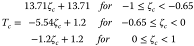
Similarly, the equations for Tb(ζb, Rd) can be given for two values of Rd following Leblanc et al. (2010):
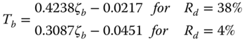
5.7.6 Load Case Scenarios Conducted by Cuéllar (2011)
Cuéllar (2011) carried out lateral load tests of a rigid monopile, running four different load case scenarios for a remarkable 5 million load cycles. The goal of the analysis was to identify qualitative trends in the strain accumulation and to analyse densification of the soil due to cyclic lateral load on the pile. It was found in their study that the plot of the accumulation of permanent deformation against the number of cycles can be approximated by three different simplified curves.
- In the first roughly 104 cycles, the accumulation follows a logarithmic curve in the form of ρ1 = C1 + C2 log(N). A quick accumulation of permanent displacements likely due to the densification around the pile is followed by a region of stabilised cyclic amplitude.
- Stabilised cyclic amplitude is characteristic of this intermediate region, where the accumulation is roughly linear with ρ2 = C3 + C4N.
- The last section after the second inflection point at roughly 106 number of cycles can be approximated by a power law curve as
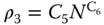 .
.
The rate of accumulation never seems to fall to zero, but the accumulated rotation appears to increase indefinitely.
5.8 Theory for Estimating Natural Frequency of the Whole System
The structural model that can be used for simplified calculations is shown in Figure 5.18. The foundation is represented by three springs: lateral KL, rotational KR, and cross KLR stiffness. The tower can be idealised by equivalent bending stiffness and mass per length. Two types of beam theory can be used: Euler‐Bernoulli beam theory and improved Timoshenko beam theory, and partial differential equations need to be used. Timoshenko beam theory accounts for shear deformation and the effect of rotational inertia, see Figure 5.45. In both the models, the rotor‐nacelle assembly (RNA) is modelled as a top head mass with mass moment of inertia.
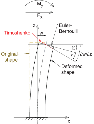
Figure 5.45 Timoshenko beam: the effect of rotary inertia and shear deformation are added to the Euler−Bernoulli beam model.
5.8.1 Model of the Rotor‐Nacelle Assembly
The RNA is modelled as a top head mass M2 with mass moment of inertia J, as shown in Figure 5.18. These parameters can be used to formulate the end boundary conditions of the PDEs of the motion of the tower. In addition, the mass M2 exerts a downwards pointing force P due to gravity, which can be considered constant along the tower:
The self‐weight of the tower also produces an axial force on the sections below;
where m is the average mass per length of the tower, L is the height of the tower, and z is the coordinate running along the tower. An approximate method is followed here as given in Adhikari and Bhattacharya (2011) and in Blevins (1979, p. 36):
where Mcorr is the corrected mass, M2 is the mass of the nacelle, M3 is the mass of the tower, and ![]() is the modified constant axial force. The mass correction factor CM = 33/140 ≈ 0.24 for a cantilever beam is given in, e.g. Blevins (1979). The mass correction factor for flexible foundation was derived in Adhikari and Bhattacharya (2012). This expression uses the nondimensional variables given in Eq. (5.45).
is the modified constant axial force. The mass correction factor CM = 33/140 ≈ 0.24 for a cantilever beam is given in, e.g. Blevins (1979). The mass correction factor for flexible foundation was derived in Adhikari and Bhattacharya (2012). This expression uses the nondimensional variables given in Eq. (5.45).
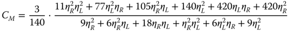
5.8.2 Modelling the Tower
Generally, if the beam is slender, the simple Euler‐Bernoulli beam model can be used, which can be improved by taking into consideration the effect of rotational inertia (Rayleigh beam). As a rule of thumb, the column can be considered as a slender beam if the length‐to‐diameter ratio is higher than about 20, and stocky when the ratio is smaller than 10, in which case the Timoshenko beam theory is necessary.
5.8.3 Euler‐Bernoulli Beam – Equation of Motion and Boundary Conditions
The equation of motion can be written as

where w(z, t) is the translational deflection of the beam at the cross‐section z at time t, EI(z) is the bending stiffness of the beam at cross section z, m(z) is the mass per length of the beam at cross section z, ![]() is the constant, corrected lumped mass at the top of the tower, and p(z, t) is an arbitrary distributed force. In the following, an equivalent bending stiffness and a constant mass per length are assumed, the notations
is the constant, corrected lumped mass at the top of the tower, and p(z, t) is an arbitrary distributed force. In the following, an equivalent bending stiffness and a constant mass per length are assumed, the notations ![]() (z, t) for derivative with respect to z and
(z, t) for derivative with respect to z and ![]() for the time derivative are introduced, the explicit notation of space and time dependence is omitted, and the variables are separating and a harmonic solution is assumed. Boundary conditions are determined considering the flexible foundation (KL, KR, and KLR) and the lumped mass and inertia (M2 and J). The readers are referred to Adhikari and Bhattacharya (2011), Arany et al. (2016), and Arany et al. (2015a,b) for details of the boundary conditions. Some details are provided in Appendices A to C.
for the time derivative are introduced, the explicit notation of space and time dependence is omitted, and the variables are separating and a harmonic solution is assumed. Boundary conditions are determined considering the flexible foundation (KL, KR, and KLR) and the lumped mass and inertia (M2 and J). The readers are referred to Adhikari and Bhattacharya (2011), Arany et al. (2016), and Arany et al. (2015a,b) for details of the boundary conditions. Some details are provided in Appendices A to C.
5.8.4 Timoshenko Beam Formulation
The classical Euler‐Bernoulli beam theory does not include the effects of shear deformation and rotary inertia, which should be included for stocky beams. The analysis was carried out for wind turbine towers for the sake of comparison to simpler beam models and to investigate whether the slender beam approximation is appropriate. The equation of motion was derived by Timoshenko and can be written with two equations as:
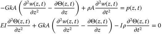
where w(z, t) is the transversal displacement in the x direction at the coordinate z at time t; ρ is the density of the material of the tower; A is the area of the cross section ![]() ; k is the Timoshenko shear coefficient; G is the shear modulus; p(z, t) is the external force; EI is the bending stiffness of the tower; E is Young's modulus;
; k is the Timoshenko shear coefficient; G is the shear modulus; p(z, t) is the external force; EI is the bending stiffness of the tower; E is Young's modulus; ![]() is the area moment of inertia of the cross section; and Θ(z, t) is the angle due to pure bending. These two equations can be transformed into one. For the natural frequency, the excitation is taken to be zero:
is the area moment of inertia of the cross section; and Θ(z, t) is the angle due to pure bending. These two equations can be transformed into one. For the natural frequency, the excitation is taken to be zero:

Using separation of variables and assuming a harmonic solution:
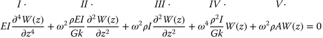
- Shear force: included in the Euler‐Bernoulli beam theory.
- Shear deformation: included in the Timoshenko beam theory. If shear deformation is to be excluded from the equation, it can be done by letting G → ∞.
- Rotary inertia: included in the Rayleigh beam theory. If rotary inertia is to be neglected, then terms containing ρI must be set equal to zero (but not ρIE).
- Coupling term between shear deformation and rotary inertia: it is only present if both effects are included.
- Force by acceleration: included in the Euler‐Bernoulli beam theory.
Using the nondimensional variable ξ = z/L and incorporating the axial loading, the following equation can be written:
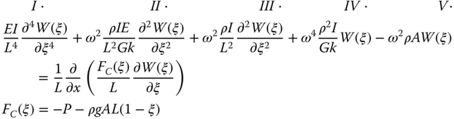
where FC(ξ) is the compressive force at each cross section.

Nondimensional parameters have been used by Arany et al. (2016) to study the problem and are shown in Table 5.16. The range of typical values (estimated based on four wind turbines) is also shown in Table 5.16 and 5.18.
Table 5.16 Nondimensional groups: definitions and practical range.
| Dimensionless group | Formula | Typical values |
| Nondimensional lateral stiffness |  |
2 500–12 000 |
| Nondimensional rotational stiffness | 25–80 | |
| Nondimensional cross stiffness | 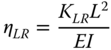 |
(−515) to (−60) |
| Nondimensional axial force | 0.005–0.1 | |
| Mass ratio |  |
0.75–1.2 |
| Nondimensional rotary inertia | a | |
| Nondimensional shear parameter | ∼4.5 (for steel tubular towers) | |
| Nondimensional radius of gyration | 0.008–0.025 | |
| Frequency scaling parameter | 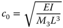 |
∼1–5 |
| Nondimensional rotational frequency | 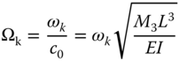 |
— |
KL, KR, KLR are the lateral, rotational, and cross stiffness of the foundation, respectively; EI is the equivalent bending stiffness of the tapered tower; L is the height of the tower; P* is the modified axial force (see Eq. 4); M2 is the total top mass (blades, hub, nacelle, etc.); M3 is the mass of the tower; J is the rotary inertia of the top mass; m is the equivalent mass per length of the tower; ![]() is the radius of gyration of the tower; ωk is the kth natural frequency of the tower.
is the radius of gyration of the tower; ωk is the kth natural frequency of the tower.
aThe rotary inertia is taken to be zero for all wind turbines considered, as information is not available in the referenced literature.
The above‐presented nondimensional numbers were determined for four offshore wind turbines, the measured and/or estimated natural frequencies of which are available in the literature. The information necessary for frequency estimation are given in Table 5.17, the nondimensional variables are calculated in Table 5.18 and the results of the proposed model are compared to available values in Table 5.18. The approximations tend to underestimate the natural frequency except for the Lely A2 wind farm, even if the foundation is infinitely stiff (fixed‐base natural frequency). It is to be noted here that the model uses a constant average thickness for the towers, determined based on the range of thickness available in the literature and the masses of the towers. Real towers tend to have thicker walls in the bottom section and thinner ones in the upper sections, which increases the tower's natural frequency as compared to a constant thickness. As the natural frequency was found to be highly sensitive to the chosen wall thickness, this parameter may be the reason behind the underestimation. There are many other sources of uncertainty, including but not limited to damping (soil, structural, aerodynamic, hydrodynamic), lengths, soil parameters and foundation stiffness, flexibility of support structure connections, and mass moment of inertia (Table 5.19).
Table 5.17 Information required for frequency estimation.
| Wind turbine | Lely A2: NM41 2‐bladed, 500 kW turbine for study purposes | North Hoyle Vestas V80 2 MW industrial wind turbine | Irene Vorrink 600 kW study purpose wind turbine | Walney 1 Siemens SWT‐3.6‐107 3.6 MW industrial wind turbine |
| Given and calculated geometric and material data | ||||
| Equivalent bending stiffness – EI (GNm) | 22 | 133 | 21.5 | 274 |
| Young's modulus of the tower material – E (GPa)] | 210 | 210 | 210 | 210 |
| Shear modulus of the tower material – G (GPa) | 79.3 | 79.3 | 79.3 | 79.3 |
| Tower height – L (m) | 41.5 | 70 | 51 | 83.5 |
| Bottom diameter – Db (m) | 3.2 | 4.0 | 3.5 | 5.0 |
| Top diameter – Dt (m) | 1.9 | 2.3 | 1.7 | 3.0 |
| Tower wall thickness range – t (mm) | ∼12 | ∼35 | …14 | 20.80 |
| Lateral foundation stiffness – KL (GN m−1) | 0.83 | 3.1…3.5 | 0.76 | 3.65 |
| Rotational foundation stiffness – KR (GNm rad−1) | 20.6 | 33.8…62.1 | 15.5 | 254.3 |
| Cross‐coupling foundation stiffness – KLR (GN) | −2.22 | −1.71 | −2.35 | −20.1 |
| Top mass (rotor‐nacelle assembly) – M2(kg) | 32 000 | 100 000 | 35 700 | 234 500 |
| Tower mass – M3 (kg) | 31 440 | 130 000 | 31 200 | 260 000 |
| Average wall thickness – th (mm) | 12 | 35 | 11 | 40 |
| Shear coefficient – k (−) | 0.532 8 | 0.532 8 | 0.532 6 | 0.532 7 |
Table 5.18 Nondimensional parameters.
| Wind turbine | Lely A2 | North Hoyle | Irene Vorrink | Walney 1e |
| Nondimensional parameters | ||||
| Nondimensional lateral stiffness – ηL | 2 698 | 11 775 | 5 880 | 7 763 |
| Nondimensional rotational stiffness – ηR | 38.88 | 28 | 39.64 | 77.49 |
| Nondimensional cross‐coupling stiffness – ηLR | −174 | −63 | −284 | −511.7 |
| Nondimensional axial force – ν | 0.033 | 0.011 | 0.030 | 0.043 |
| Mass ratio – α | 1.018 | 0.760 | 1.144 | 0.9 |
| Nondimensional rotary inertia – β | 0 | 0 | 0 | 0 |
| Frequency scaling parameter – c0 | 3.130 | 1.323 | 2.035 | 1.345 4 |
| Nondimensional radius of gyration – μ | 0.021 4 | 0.016 1 | 0.017 95 | 0.016 8 |
| Nondimensional shear parameter – γ | 4.970 | 4.970 | 4.970 | 4.97 |
Table 5.19 Frequency results.
| Wind turbine | Lely A2 | North Hoyle | Irene Vorrink | Walney 1 |
| Natural frequency results | ||||
| Measured value – fm (Hz) | 0.634 | N/A | 0.546 | 0.35 |
| Result produced by [28] – fS (Hz) | 0.740 | 0.345 | 0.457 | — |
| Present study (Euler‐Bernoulli) – fE − B (Hz) (error [%]) | 0.735 (15.9%) | 0.345 (N/A) | 0.456 (16.5%) | 0.331(5.9%) |
| Present study (Timoshenko) – fT (Hz) (error[%]) | 0.734 (15.8%) | 0.345 (N/A) | 0.456 (16.5%) | 0.331(5.9%) |
| Fixed‐base frequency (infinitely stiff foundation) | 0.765 | 0.364 | 0.475 | 0.345 |
5.8.5 Natural Frequency versus Foundation Stiffness Curves
Figure 5.46 plots the relationship between two non‐dimensional support stiffness (ηL and ηR) and the relative frequency for various values of cross‐coupling stiffness (KLR). It can be concluded from these graphs that with the increase of the cross‐spring stiffness, the OWT is closer to the high‐slope zone of the curves. In such circumstances, the changes in the stiffness parameters introduce a higher change in natural frequency. In Figures 5.47–5.49, the same four turbines are placed in the relative frequency figures with respect to the three stiffness parameters. Each line style shows the relative frequency curve of a given OWT, and the estimated values on the curves are also shown for each turbine. In general, the sensitivity of the natural frequency to each parameter may be characterised by the slope of the curve at the estimated stiffness values.
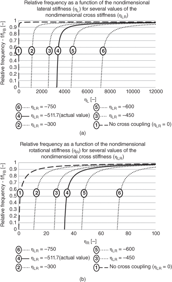
Figure 5.46 .Relative frequency as a function of (a) the nondimensional lateral stiffness, (b) the nondimensional rotational stiffness for several values of the nondimensional cross stiffness.
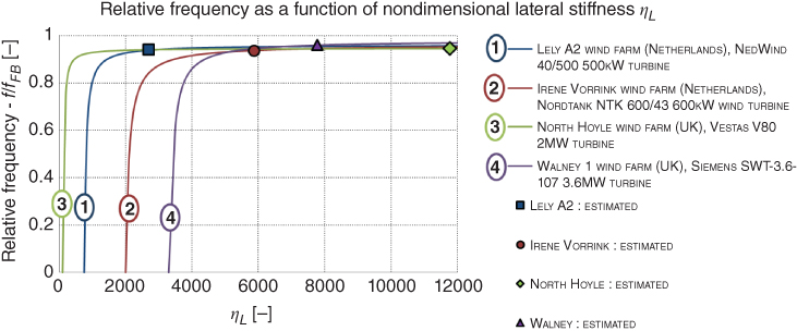
Figure 5.47 Relative frequency  as a function of the nondimensional lateral stiffness
  .
.
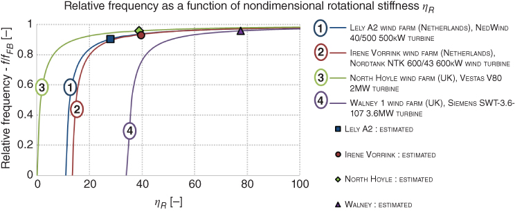
Figure 5.48 Relative frequency  as a function of the nondimensional rotational stiffness
  .
.
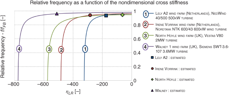
Figure 5.49 Relative frequency fr = f/fFB as a function of the nondimensional cross stiffness ηLR = KRL2/EI.
One of the main purposes of SSI analysis is to study the effect of change of soil parameters during the operation of the turbine, i.e. how much the frequency will change if soil softens or stiffens due to repeated cyclic loading. This change in foundation stiffness has been reported in small‐scale tests and observed in the case of the Hornsea Met Mast Twisted Jacket foundation. A few design pointers may be deduced from the study:
- From a design point of view, it is important to note that the nondimensional stiffness values have a certain region where the frequency function becomes flat, i.e. any change in foundation stiffness will have very little impact on the natural frequency. The designer may wish to choose the tower stiffness (EI) and foundation stiffness (KL, KR, and KLR) such as to remain in the safe region to ensure that even if the stiffness parameters change during the lifetime of the turbine, the natural frequency will not be greatly affected.
- It can be observed that the structures are relatively insensitive to the lateral stiffness (KL) and the most important factor is the rotational stiffness (KR). In general, one can conclude that the change in rotational stiffness of the foundation causes the greatest change in natural frequency.
- The cross stiffness (KLR) also has important effects and may not be neglected.
5.8.6 Understanding Micromechanics of SSI
The readers are referred to the work of Cui and Bhattacharya (2017) and Lopez Querol et al. (2017) where discrete element modelling of the monopile‐soil interaction has been studied.
Chapter Summary and Learning Points
- SSI governs the long‐term performance of the wind turbine system. The issues affecting a monopile foundation are the extreme wind and wave loading, cyclic and dynamic loading, and soil erosion.
- The change in natural frequencies of the wind turbine system may be affected by the choice of foundation system, i.e. deep foundation or multiple pods on shallow foundations. Deep foundations such as monopiles will exhibit sway‐bending mode, i.e. the first two modes are widely spaced. However, multiple pod foundations supported on shallow foundations (such as tetrapod or tripod on suction caisson) will exhibit rocking modes in two principal planes.
- The natural frequencies of wind turbine systems change with repeated cyclic/dynamic loading. In the case of a strain‐hardening site (such as loose to medium‐dense sandy site) the natural frequency is expected to increase, and for strain‐softening site (such as normally consolidated clay) the natural frequency will decrease.
- Due to the rocking modes of vibration, there will be a ‘two‐peak’ response, i.e. two closely spaced frequencies for multipod foundations (tripod/tetrapod).