
2
Loads on the Foundations
2.1 Dynamic Sensitivity of Offshore Wind Turbine Structures
Offshore wind turbines (OWTs), due to their shape and form (slender column with a heavy mass as well as a rotating mass at the top), are dynamically sensitive. The natural frequency of these slender structures is very close to the excitation frequencies imposed by the environmental and mechanical loads. The aim of the foundation is to transfer the loads of the substructure and superstructure safely to the ground. This chapter reviews the loads acting on the wind turbine structure. Apart from the self‐weight of the whole system, there are four main lateral loads acting on an OWT structure: wind, wave, 1P (rotor frequency), and 2P/3P (blade‐passing frequency) loads.
The main cyclic/dynamic loads acting on the wind turbine are as follows:
- Wind. The load produced by the thrust of the wind on the blades and tower. The cyclic component of the load depends on the turbulence of the wind at that location (wind speed variation over a period) and turbine operating characteristics.
- Wave. The load caused by waves crashing against the substructure (i.e. the part of the structure exposed to the wave), the magnitude of which depends on the wave height and wave period;
- 1P load. Load caused by the vibration at the hub level due to the mass and aerodynamic imbalances of the rotor. This load has a frequency equal to the rotational frequency of the rotor (referred to as 1P loading). Since most of the industrial wind turbines are variable‐speed machines, 1P is not a single frequency but a frequency band between the frequencies associated with the lowest and the highest rpm (revolutions per minute). Ranges of typical 1P frequencies for different wind turbines are given in Chapter 1 (Table 1.1) and are noted by cut‐in (RPM) and ‘rated (RPM)’.
- Blade‐passing load (2P/3P). Loads in the tower due to the vibrations caused by blade shadowing effects (referred to as 2P/3P). As the blades of the turbine pass through the front of the tower, the temporary shadowing effect reduces the thrust on the tower. Figure 2.1 shows the shadowing effect due to two configurations of the blades, and the differential load on the tower may be noted. This is a dynamic load having frequency equal to three times the rotational frequency of the turbine (3P) for three‐bladed wind turbines. For a two‐bladed turbine, this will be two times (2P) the rotational frequency of the turbine (1P). The 2P/3P loading is also a frequency band like 1P and is simply obtained by multiplying the limits of the 1P band by the number of the turbine blades.

Figure 2.1 Explanation of 3P loading.
2.2 Target Natural Frequency of a Wind Turbine Structure
To ascertain if the loads are dynamic and to estimate them, one needs to find the frequency of the load as well as that of the structure. One of the first steps in a design is to fix the target frequency of the whole wind turbine structure. Figure 2.3 shows a mechanical model of a monopile‐supported wind turbine structure that can be used to estimate the natural frequency of the structure. In the model, the foundation is replaced by a set of springs and is often known as macro‐element model. Based on a pile geometry and ground profile (i.e. ground stiffness along the depth of the ground), one can obtain the initial stiffness of the foundation( i.e. KL, KR, and KLR). Methods to estimate these are explained in Chapter 5 and worked examples are provided in Chapter 6. KL represents lateral stiffness i.e. force required for unit lateral displacement of the pile head (unit of MN m−1), whereas KR represents moment required for unit rotation of the pile head (unit of GNm rad−1). KLR is the cross‐coupling spring and will be explained in subsequent chapters. Once KL, KR, and KLR are known, one can predict the first natural frequency of the whole system for sway‐bending modes. KV is the vertical stiffness of the foundation and is necessary for axial vibration analysis.
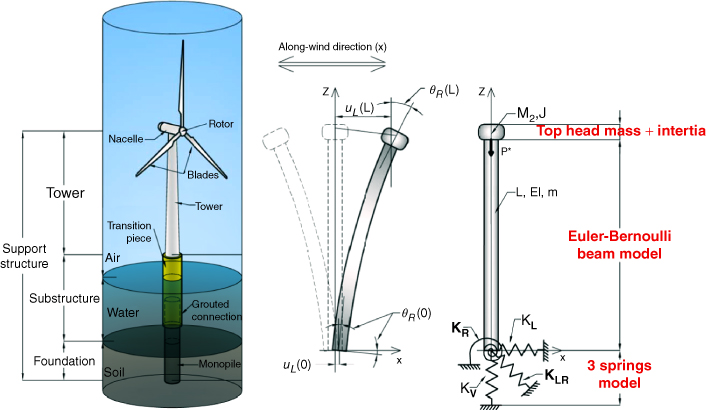
Figure 2.3 Simplified diagram of a wind turbine structure.
The target frequency of the whole system depends on the location and the turbine used: wind turbulence information, wave period, and spectrum as well as operating range of the turbine (1P range). The turbulent wind velocity and the wave height on sea are both variables and are best treated statistically using power spectral density (PSD) functions. In other words, instead of time domain analysis the produced loads are more effectively analysed in the frequency domain, whereby the contribution of each frequency to the total power in wind turbulence and in ocean waves is described. Representative wave and wind (turbulence) spectra can be constructed by a Discrete Fourier Transform (DFT) from site‐specific data. However, in the absence of such data, theoretical spectra can also be used. Some codes of practice specify Kaimal spectrum for wind and the JONSWAP (Joint North Sea Wave Project) spectrum for waves. Details on the construction of wind and wave spectrum are provided in the next few sections.
Figure 2.4 plots a schematic PSD function for typical wind and waves. The figure also shows the 1P and 3P frequency bands, which depend on the range of 1P frequency. It is obvious to avoid the excitation frequencies from resonance point of view. Det Norske Veritas (DNV) code suggests that first natural frequency should not be within 10% of the 1P and 3P ranges and is indicated as ‘safety margin’ in Figure 2.4. It is therefore clear that the first natural frequency of the wind turbine needs to be fitted in a very narrow band. For some cases, 1P and 3P ranges may even coincide, leaving no gap, and in such cases, the control system is designed to leapfrog some frequencies in 1P range.
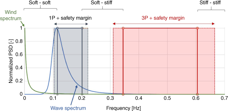
Figure 2.4 Range of frequencies acting on a wind turbine structure.
Design is therefore a collaborative effort between turbine manufacturer and substructure designer. In the current practice, the turbine manufacturer will provide the detailed design of the tower and the RNA. The substructure designer will carry out the design of transition piece and the foundation.
It is clear from the frequency content of the applied loads that the designer has to select a system frequency i.e. global frequency of the overall wind turbine including the foundation, which lies outside these frequencies to avoid resonance and ultimately increased fatigue damage. From the point of view of first natural frequency f0 of the structure, three types of designs are possible:
- Soft‐soft design where f0 is placed below the 1P frequency range (f0 < f1P, min) , which is a very flexible structure and almost impossible to design for a grounded system.
- Soft‐stiff design where f0 is between 1P and 3P frequency ranges (f1P, max < f0 < f3P, min) and this is the most common in the current offshore development.
- Stiff‐stiff designs where f0 have a higher natural frequency than the upper limit of the 3P band (f0 > f3P, max) and will need a very stiff support structure.
It is important to note that from the point of view of dynamics, OWT designs are only conservative if the prediction of the first natural frequency are sufficiently accurate. Unlike in the case of some other offshore structures (such as the ones used in the oil and gas industry), under‐prediction of f0 is unconservative. The safest solution would seem to be placing the natural frequency of the wind turbine well above the 3P range. However, stiffer designs with higher natural frequency require massive support structures and foundations involving higher costs of materials, transportation, and installation. Thus, from an economic point of view, softer structures are desirable, and it is not surprising that almost all of the installed wind turbines are ‘soft‐stiff’ designs, and this type is expected to be used in the future as well. It is clear from the above discussion that designing soft‐stiff wind turbine systems demands the consideration of dynamic amplification and also any potential change in system frequency due to the effects of cyclic/dynamic loading on the system i.e. dynamic‐structure‐foundation‐soil‐interaction.
2.3 Construction of Wind Spectrum
Turbulence of wind is usually estimated as a fluctuating wind speed component (u) superimposed on the mean wind speed ![]() , and therefore the total wind speed can be written as
, and therefore the total wind speed can be written as ![]() . The degree of turbulence is usually characterised by the turbulence intensity I, given by Eq. (2.2).
. The degree of turbulence is usually characterised by the turbulence intensity I, given by Eq. (2.2).
where σU is the standard deviation of wind speed around the mean ![]() (which is usually taken over 10 minutes). The turbulence intensity varies with mean wind speed, with site location, and with surface roughness, and is also modified by the turbine itself.
(which is usually taken over 10 minutes). The turbulence intensity varies with mean wind speed, with site location, and with surface roughness, and is also modified by the turbine itself.
Taylor (1938) states in his frozen turbulence hypothesis that the characteristics of eddies can be considered constant (frozen) in time, and vortices travel with the mean horizontal wind speed as shown in Figure 2.7. This assumption is found to be acceptable for wind turbine applications, and the turbulence is usually analysed in the frequency domain by a PSD function, which describes the contribution of different frequencies to the total variance of the wind speed. The frequency of turbulence is connected to the size of eddies. A larger eddy means low‐frequency variation in wind speed, while smaller vortices induce short, high‐frequency wind‐speed variations. If characteristic size of an eddy is d[m] and it travels with ![]() speed, the travel time through the rotor in
speed, the travel time through the rotor in ![]() time. The frequency connected to this time period is f = 1/τ[Hz].
time. The frequency connected to this time period is f = 1/τ[Hz].
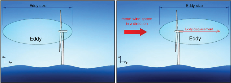
Figure 2.7 Taylor's frozen turbulence hypothesis: an eddy travels with the mean wind speed while its size and characteristic parameters remain constant.
Through this, the length scale and time scale of turbulence can be connected. The typical length scales of high energy‐containing large turbulent eddies are in the range of several kilometres. The large eddies tend to decay to smaller and smaller eddies with higher frequencies as turbulent energy dissipates to heat. Kolmogorov's law describing this process states that the asymptotic limit of the spectrum is f −5/3 at high frequency.
There are two families of spectra commonly used in wind energy applications: the von Kármán and the Kaimal spectra. The main difference is that the Kaimal spectrum is somewhat less peaked and the energy is contained in a bit wider frequency range. Kaimal spectrum is more suitable for modelling the atmospheric boundary layer, and the von Kármán spectrum is better for wind tunnel modelling. International Electrotechnical Commission (IEC) code suggests using the Mann spectrum (modified von Kármán type spectrum) and the Kaimal spectrum. On the other hand, DNV suggests the Kaimal spectrum, and it is used throughout this book. There are also other spectra, such as Froya, shown in Figure 2.5.
2.3.1 Kaimal Spectrum
Some relevant details of Kaimal spectrum connected to foundation design are given in this section:
- The power spectrum of turbulence can be modified by the landscape. If the inhomogeneity of the surface is high, the turbulence intensity increases. Another important aspect is whether the stratification is stable, unstable, or neutral. Neutral conditions rarely occur, but near‐neutral conditions are typical for medium and high wind speeds and are necessary for fatigue damage calculation.
- The theoretical Kaimal spectrum for a fixed reference point in space in neutral stratification of the atmosphere Suu(f ) as suggested by DNV can be written as:
2.3

where Lk is the integral length scale (formula available in the DNV code), f is frequency,
 is the mean wind speed (from site measurements), and σU is the standard deviation of wind speed. These can be estimated from measurements or calculated using Eq. ( 2.2), and turbulence intensity values may be obtained from standards IEC 61400‐1 and IEC 61400‐3.
Based on the DNV code, Lk = 5.67z for z < 60m and, Lk = 340.2m for z ≥ 60m where z denotes the height above sea level.
Figure 2.8 shows a comprehensive wind spectrum following van der Hoven where both long‐term variations of wind speed and turbulence effects are plotted. van der Hoven observed a significant four‐day synoptic peak and in some cases a small diurnal peak in the spectrum of the horizontal wind speed. The Kaimal spectrum describes wind turbulence on a short time scale (shown by a dotted line in Figure 2.8). This represents only the high‐frequency end of the spectrum, omitting the diurnal and synoptic peaks. Therefore, even though the Kaimal spectrum can be calculated for arbitrarily low frequency, its validity is limited to the high‐frequency variations. The lowest frequency that is typically considered corresponds to the time interval of 10 minutes, because the mean is taken over 10 minutes and therefore (T = 600 [s] → f = 1/600[Hz] ≈ 0.0017[Hz]).
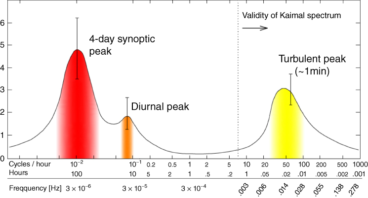
Figure 2.8 Van der Hoven spectrum and the validity of the Kaimal spectrum.
A small local gust (say of 20 m diameter) passing through the rotor has little or no effect on distant parts of the rotor area. Referring to Figure 2.9, the wind speeds of points A and B are closely related, and they show a high coherence, while a distant point, such as C in the figure, has a low coherence with either A or B. In other words, low‐frequency variations affect a larger area of the rotor than high‐frequency variations. It should also be noted that through their rotary motion the blades experience a different spectrum from the Kaimal spectrum for a point in space. The blade will pass through any given eddy once in every revolution. In Figure 2.9, Blade I, for example, passes through Eddy 1 and Eddy 2 once in each revolution. Therefore, when rotational sampling is considered, that is, the wind speed ‘seen’ by the rotating blade is sampled, the PSD will show peaks at the rotational frequency f1P and at higher harmonics ![]() . This effect is more important for blade load analysis; usually, only higher harmonics are transferred to the hub, as typically all blades pass through the same eddies.
. This effect is more important for blade load analysis; usually, only higher harmonics are transferred to the hub, as typically all blades pass through the same eddies.
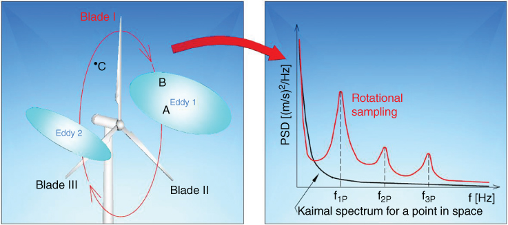
Figure 2.9 Coherence: Coherence between points A and B is high, while between C and either A or B the coherence is small. Rotational sampling: the PSD of the wind speed ‘seen’ by Blade 1 while rotating differs from the Kaimal spectrum for a point in space. The graph is a schematic representation of the PSD of rotational sampling.
Other available design wind spectra are Davenport (1961), Simiu and Leigh (1984), and Ochi and Shin (1988). For example, Ochi and Shin (1988) empirically derived a spectrum describing the wind over a sea based on offshore observations.
2.4 Construction of Wave Spectrum
The wind blowing over the sea generates wind waves because of the increased pressure on the free surface of water. First, small waves are produced with high frequency and low wave height, and the energy is gradually transferred towards the higher amplitude waves with lower frequency and longer wavelength. The developing sea state depends on many factors, including but not limited to the water depth, the shape of the sea bottom, the mean wind speed, and the fetch. The latter is the typical leeward distance to shore considering the prevailing wind direction. The dependence on the water depth is apparent from the dispersion relation:
where ω[rad/s] is the angular frequency, k = 2π/λ[1/m] is the wave number with λ[m] being the wavelength, and S[m] is the mean sea depth.
Any offshore location consists of a large number of waves with various frequencies and wavelengths. The importance of each frequency is characterised by the power associated with it, which is represented by the PSD function as shown in Figure 2.5. The PSD can be produced from site measurements of the wave height using DFT, or alternatively the JONSWAP spectrum Sww(f ) suggested by many codes such as DNV:
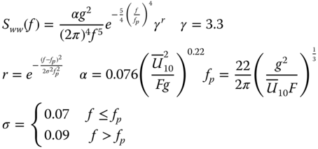
where
- f is frequency,
- α is the intensity of the spectrum,
- F is the fetch,
- fp is the peak frequency,
- γ is the peak enhancement factor,
- g is the gravitational constant,
 is the mean wind speed at 10 m height above sea level.
Both JONSWAP spectrum as well as Pierson‐Moskowitz spectrum represents the frequency content of a sea state developed in a constant wind speed condition after a sufficiently long time. The Pierson‐Moskowitz spectrum assumes a fully developed sea, and that the process of transferring energy from high to low‐frequency waves and the wave‐wave interaction have reached a steady state. Furthermore, the waves are in equilibrium with the wind. This assumption requires a sufficiently long fetch (i.e. about 5000 wavelengths), and that the constant wind velocity has maintained for sufficiently long time (i.e. about 10000 wave periods). JONSWAP spectrum takes fetch into account and thus considers a developing sea and as a result the peak frequency of the spectrum depends on the mean wind speed and the fetch. The longer the fetch, the more developed the sea is and the more energy is in the low‐frequency waves. The fetch can greatly differ for offshore wind farms located in different coasts. Figure 2.7 shows a relatively sheltered sea location where the sea is typically not fully developed. A schematic wind rose is placed at the location of the turbine.
2.4.1 Method to Estimate Fetch
A method to estimate the fetch is to take the average of the distances to leeward shores (e.g. FS, FSSW, FSW, etc.), adding weights to the distances based on the significance of the direction. For example, in Figure 2.10, the prevailing wind is blowing from south‐southwest (SSW) and southwest (SW); therefore, the weights of the distances FSSW, FSW will be the highest in the weighted average of the distances Fi.
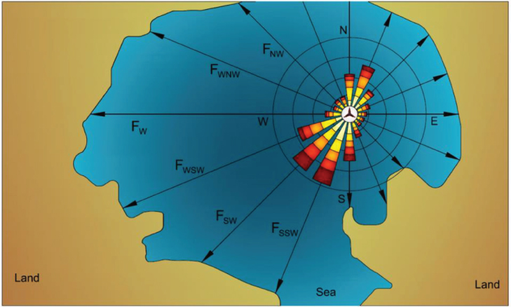
Figure 2.10 Estimation of the fetch Fi where i represents the directions of the 16‐point compass rose (e.g. S for south, SW for southwest, SSW for south‐southwest, etc.).
2.4.2 Sea Characteristics for Walney Site
Figure 2.11 shows the significant wave height (Figure 2.11a) and the peak wave period (Figure 2.11b), as functions of the mean wind speed for Walney 1 wind farm location. Curves (1)–(5) represent the JONSWAP spectrum for increasing mean wind speed and for different fetch. On the other hand, curve (6) shows the Pierson‐Moskowitz spectrum. Curves (1)–(5) in Figure 2.12a show the JONSWAP spectrum for increasing mean wind speeds keeping the fetch constant at 60[km], while curves (1)–(5) in Figure 2.12b presents the JONSWAP spectrum for increasing fetch, keeping the mean wind speed constant at 10 [m s−1].
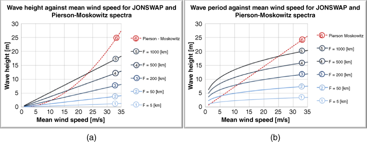
Figure 2.11 Wave height and wave period as a function of mean wind speed based for Walney 1 site. The water depth is taken as 21.5 m.
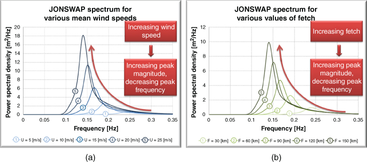
Figure 2.12 (a) JONSWAP spectrum for several values of the mean wind speed with a constant fetch of 60 km. (b) JONSWAP spectrum for several values of fetch F keeping the wind speed constant at 10 m s−1.
2.4.3 Walney 1 Wind Farm Example
Figure 2.13 shows the main frequencies from a three‐bladed Siemens 3.6 MW wind turbine having a rotational operating interval of 5–13 RPM (lowest is 5RPM i.e. 0.083 Hz and rated is 13RPM i.e. 0.216 Hz). The site is characterised by a mean wind speed of 9 m s−1 and has a peak wave frequency of 0.197 Hz. This example considers Kaimal spectrum for wind and JONSWAP spectra for wave. Details of the calculations are provided later in the chapter and in Chapter 6.
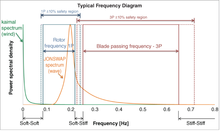
Figure 2.13 Frequency diagram for Siemens SWT‐107‐3.6 offshore wind turbine with operating rotational wind speed range between 5 and 13 rpm (using the mean wind speed U = 9 m/s and fetch F = 60 km. The frequency diagram includes wind spectrum, wave spectrum, and 1P and 3P frequency bands. The amplitudes are normalised to unity to focus on the frequency content of the loading.
2.5 Load Transfer from Superstructure to the Foundation
The loads on the foundation depend on the foundation system. In this chapter, three distinct cases are presented: (i) single foundation for a grounded system, for example monopile, mono‐caisson or a Gravity Base; (ii) multiple foundation for a grounded system; (iii) foundation for a particular floating system. The difference between the load transfer processes of single foundations and multiple foundations is explained through Figure 2.14 by taking the example of the single large diameter monopile and multiple piles supporting a jacket. In the case of monopile‐supported wind turbine structures or, for that matter, any single foundation, the load transfer is mainly through overturning moments where the monopile/foundation transfers loads to the surrounding soil and therefore there is lateral foundation−soil interaction. On the other hand, for multiple support structure, the load transfer is mainly through push‐pull action − i.e. axial load, as illustrated in the figure.
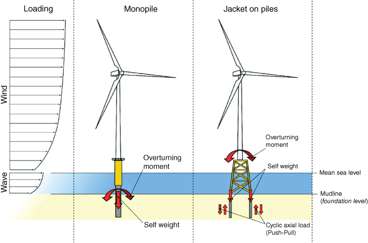
Figure 2.14 Load transfer for monopile‐supported and multiple‐foundation‐supported foundations.
Figure 2.15 shows a particular type of floating system known as spar‐supported floating OWTs with catenary mooring and suction caisson anchors. This is effectively the example of the Hywind concept, the first floating offshore wind farm. For foundation design, it is necessary to estimate an upper bound for the ultimate load on the anchor. This can be obtained by taking the configuration where the mooring line is completely stretched and there is no part of it lying on the seabed. This is very similar to the configuration of a single taut mooring line. In this case the load is transferred directly to the anchor without the effect of soil friction on a horizontal section of the mooring line. Furthermore, in this configuration the angle of the mooring line at the seabed is also maximal, which impacts the inverse catenary shape at the anchor. This configuration is also shown in Figure 2.15. This is very similar to the broken line configuration scenario for the case of FPSO (floating production storage and offloading) anchor design; see Bhattacharya et al. (2006).
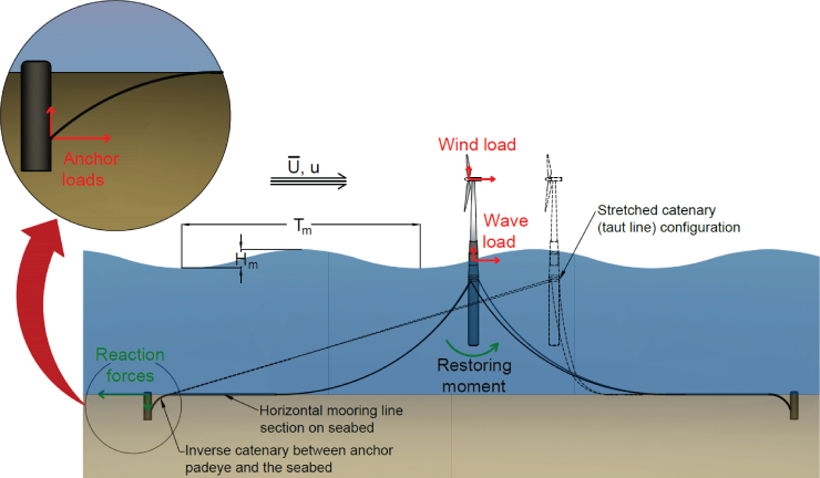
Figure 2.15 Load transfer for floating offshore wind turbine system.
2.6 Estimation of Loads on a Monopile‐Supported Wind Turbine Structure
The loads acting on the wind turbine rotor and substructure are ultimately transferred to the foundation and can be classified into two types: static or dead load due to the self‐weight of the components and the cyclic/dynamic loads arising from the wind, wave, and 1P and 3P loads. However, the challenging part is the dynamic loads acting on the wind turbine and the salient points are as follows:
- The rotating blades apply a cyclic/dynamic lateral load at the hub level (top of the tower), and this load is determined by the turbulence intensity in the wind speed. The magnitude of the dynamic load component depends on the turbulent wind speed component.
- The waves crashing against the substructure apply a lateral load close to the foundation. The magnitude of this load depends on the wave height and wave period, as well as the water depth.
- The mass imbalance of the rotor and hub and the aerodynamic imbalances of the blades generate vibration at the hub level and apply lateral load and overturning moment. This load has a frequency equal to the rotational frequency of the rotor (referred to as 1P loading in the literature). Since most industrial wind turbines are variable speed machines, 1P is not a single frequency but a frequency band between the frequencies associated with the lowest and the highest rpm (revolutions per minute).
- The blade‐shadowing effects (referred to as 2P/3P in the literature) also apply loads on the tower. This is a dynamic load having frequency equal to three times the rotational frequency of the turbine (3P) for three‐bladed wind turbines and two times (2P) the rotational frequency of the turbine for two‐bladed turbines. Rotational sampling of the turbulence by the blades and wind shear may also produce 2P/3P loads at the foundation. The 2P/3P excitations also act in a frequency band like 1P and are simply obtained by multiplying the limits of the 1P band by the number of the turbine blades.
This section presents a calculation procedure that can be easily carried out in a spreadsheet program. The output of such a calculation will be relative wind and the wave loads. For simplified design purposes, it is assumed that the wind and wave are perfectly aligned. This is a fair assumption for deeper water further offshore projects where the fetch distance is high.
The peak frequency of the wind turbulence can be obtained theoretically from the Kaimal spectrum. In the absence of site‐specific data, and for foundation design purposes, the wind load can be assumed to act at the hub level with a time period for wind given by ![]() (where Lkis the integral length scale and
(where Lkis the integral length scale and ![]() is the wind speed) and typical values are about 100 seconds.
is the wind speed) and typical values are about 100 seconds.
2.6.1 Load Cases for Foundation Design
IEC codes (IEC 2005; IEC 2009a; IEC 2009b) as well as the DNV code (DNV 2014) describe hundreds of load cases that need to be analysed to ensure the safe operation of wind turbines throughout their lifetime of 20–30 years. However, in terms of foundation design, not all these cases are significant or relevant. The main design requirements for foundation design as will be explained in Chapter 3are ULS (Ultimate Limit State), FLS (Fatigue Limit State), and SLS (Serviceability Limit State). Five load cases important for simplified foundation design are identified and described in Table 2.1.
Table 2.1 Representative design environmental scenarios as load cases chosen for foundation design.
| # | Name and description | Wind model | Wave model | Alignment |
| E‐1 |
Normal operational conditions Wind and wave act in the same direction (no misalignment). |
NTM at UR (U‐1) | 1‐yr ESS (W‐1) | Collinear |
| E‐2 |
Extreme wave load scenario Wind and wave act in the same direction (no misalignment). |
ETM at UR (U‐2) | 50‐yr EWH (W‐4) | Collinear |
| E‐3 |
Extreme wind load scenario Wind and wave act in the same direction (no misalignment). |
EOG at UR (U‐3) | 1‐yr EWH (W‐2) | Collinear |
| E‐4 | Cut‐out wind speed and extreme operating gust scenario Wind and wave act in the same direction (no misalignment). | EOG at Uout (U‐4) | 50‐yr EWH (W‐4) | Collinear |
| E‐5 |
Wind‐wave misalignment scenario Same as E‐2, except the wind and wave are misaligned at an angle of φ = 90°. The dynamic amplification is higher in the cross‐wind direction due to low aerodynamic damping. |
ETM at UR (U‐2) | 50‐yr EWH (W‐4) | Misaligned at φ = 90° |
All design load cases are built as a combination of four wind and four sea states. The wind conditions are:
- (U-1) Normal turbulence scenario. The mean wind speed is the rated wind speed (UR) where the highest thrust force (Th) is expected, and the wind turbulence is modelled by the Normal Turbulence Model (NTM). The NTM standard deviation of wind speed is defined in IEC (2005).
- (U-2) Extreme turbulence scenario. The mean wind speed is the rated wind speed (UR), and the wind turbulence is very high. The extreme turbulence model (ETM) is used. The ETM standard deviation of wind speed is defined in IEC (2005).
- (U-3) Extreme gust at rated wind speed scenario. The mean wind speed is the rated wind speed (UR) and the 50‐year extreme operating gust (EOG) calculated at UR hits the rotor. The EOG is a sudden change in the wind speed and is assumed to be so fast that the pitch control of the wind turbine has no time to alleviate the loading. This assumption is very conservative and is suggested to be used for simplified foundation design. The EOG speed is defined in IEC (2005).
- (U-4) Extreme gust at cut‐out scenario. The mean wind speed is slightly below the cut‐out wind speed of the turbine (Uout) and the 50‐year EOG hits the rotor. Due to the sudden change in wind speed the turbine cannot shut down. Note that the EOG speed calculated at the cut‐out wind speed is different from that evaluated at the rated wind speed (IEC 2005).
The wave conditions are:
- (W-1) One‐year extreme sea state (ESS). A wave with height equal to the 1‐year significant wave height HS, 1 acts on the substructure.
- (W-2) One‐year extreme wave height (EWH). A wave with height equal to the 1‐year maximum wave height Hm, 1 acts on the substructure.
- (W-3) 50‐year ESS. A wave with height equal to the 50‐year significant wave height HS, 50 acts on the substructure.
- (W-4) 50‐year EWH. A wave with height equal to the 50‐year maximum wave height Hm, 50 acts on the substructure.
The one‐year ESS and EWH are used as a conservative overestimation of the normal wave height (NWH) prescribed in IEC (2009a). It is important to note here in relation to the ESS that the significant wave height and the maximum wave height have different meanings. The significant wave height HS is the average of the highest one‐third of all waves in the three‐hour sea state, while the maximum wave height Hm is the single highest wave in the same three‐hour sea state.)
According to the relevant standards (IEC 2005; IEC 2009a; DNV 2014), in the probability envelope of environmental states the most severe states with a 50‐year return period has to be considered, and not 50‐year return conditions for wind and wave unconditionally (separately). Indeed, extreme waves and high wind speeds tend to occur at the same time; however, the highest load due to wind is not expected when the highest wind speeds occur. This is partly because the pitch control alleviates the loading above the rated wind speed, but also because turbines shut down at high wind speeds for safety reasons. Idle or shut‐down turbines, as well as turbines operating close to the cut‐out wind speed have a significantly reduced thrust force acting on them compared to the thrust force at the rated wind speed due to the reduced thrust coefficient, as shown in Figures 2.17 and 2.18.
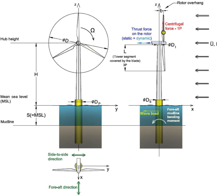
Figure 2.16 Definition of the geometry, axes, loads, and directions of the offshore wind turbine structure.
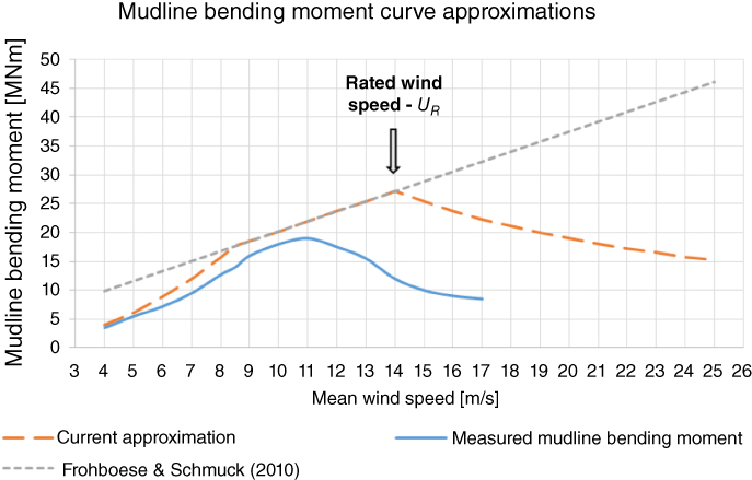
Figure 2.17 Measured and approximated mudline bending moments of Horns Rev offshore wind turbine. The measured data are obtained from Hald et al. (2009).
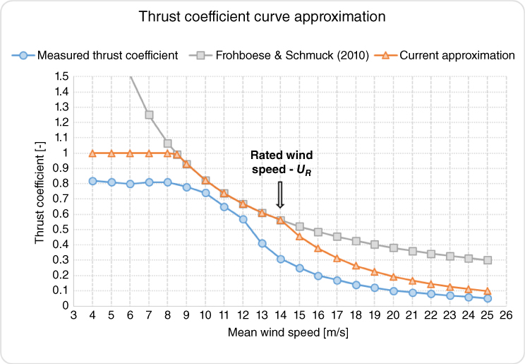
Figure 2.18 Measured (Hald et al. 2009) and approximate thrust coefficients of the Vestas V80 turbine at Horns Rev.
The highest wind load is expected to be caused by scenario U‐3 and the highest wave load is due to scenario W‐4. In practice, the 50‐year extreme wind load and the 50‐year extreme wave load have a negligible probability to occur at the same time, and the DNV (2014) code also doesn't require these extreme load cases to be evaluated together. The designer has to find the most severe event with a 50‐year return period based on the joint probability of wind and wave loading. Therefore, for the ULS analysis (for details see Chapter 3), two combinations are suggested by Arany et al. (2017):
- The ETM wind load at rated wind speed combined with the 50‐year EWH – the combination of wind scenario U‐2 and wave scenario W‐4. This will provide higher loads in deeper water with higher waves.
- The 50‐year EOG wind load combined with the one‐year maximum wave height. This will provide higher loads in shallow water in sheltered locations where wind load dominates.
These scenarios are somewhat more conservative than those required by standards, and can be adopted for simplified analysis. From the point of view of SLS and FLS, the single largest loading on the foundation is not representative, because the structure is expected to experience this level of loading only once throughout the lifetime.
The load cases in Table 2.1 are considered to be representative of typical foundation loads in a conservative manner and may serve as the basis for conceptual design of foundations. However, detailed analysis for design optimization and the final design may require addressing other load cases as well. These analyses require detailed data about the site (wind, wave, current, geological, geotechnical, bathymetry data, etc.) and also the turbine (blade profiles, twist and chord distributions, lift and drag coefficient distributions, control parameters and algorithms, drive train characteristics, generator characteristics, tower geometry, etc.).
2.6.2 Wind Load
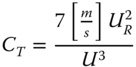
The thrust force (Th) on a wind turbine rotor due to wind can be estimated in a simplified manner as
where ρa is the density of air, AR is the rotor swept area, CT is the thrust coefficient, and U is the wind speed. The wind speed can range from cut‐in to cut‐out, with the appropriate thrust coefficient. The thrust coefficient can be approximated in the operational range of the turbine using three different sections (as shown in Figures 2.16 and 2.17):
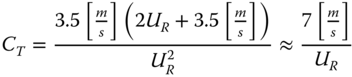
- Between cut‐in (Uin) and rated wind speed (UR), the method of Frohboese and Schmuck (2010) is recommended following Arany et al. (2017)2.7
- After rated wind speed, when the pitch control is active, the power is assumed to be kept constant, and thus the thrust coefficient is expressed as2.8
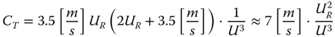
- The thrust coefficient is assumed not to exceed 1; therefore, in the low‐wind‐speed regime where the formula of Frohboese and Schmuck (2010) overestimates the thrust coefficient, the value is capped at 1.
When the wind speed is changing slowly, the thrust force follows the mean thrust curve as the pitch control follows the change in wind speed. However, when a sudden gust hits the rotor, the pitch control's time constant might be too high to follow the sudden change. If this is the case, then the thrust coefficient is ‘locked’ at its previous value while the wind speed in Eq. (2.11) changes to the increased wind speed due to the gust.
Assuming a quasi‐static load calculation method, the wind speed can be divided into two parts, a mean wind speed ![]() , and a turbulent wind speed u component. For each load case, the mean wind speed
, and a turbulent wind speed u component. For each load case, the mean wind speed ![]() and the turbulent wind speed component u are defined separately, and the total wind speed is expressed as
and the turbulent wind speed component u are defined separately, and the total wind speed is expressed as
Using this assumption, the wind load can be separated into a mean thrust force (or static force) and a turbulent thrust force (or dynamic force).
In this equation, the thrust coefficient CT is calculated as shown in Eq. ( 2.11).
2.6.2.1 Comparisons with Measured Data
Figure 2.17 plots the measured mean mudline‐bending moment for a Vestas V80 wind turbine at the Horns Rev offshore wind farm obtained from Hald et al. (2009) and compares it with the approximation based on Eq. (2.10). This is based on the measured thrust force acting at the hub level, and the corresponding thrust coefficient is shown in Figure 2.18.
The maximum thrust force occurs around the rated wind speed (or, more specifically, before the pitch control activates). In reality, the pitch control activates somewhat below the rated wind speed (as can be seen in Figures 2.17 and 2.18). This is to ensure a smooth transition between the section where the power is proportional to the cube of the wind speed and the pitch controlled region where the power is kept constant to avoid repeated switching around the rated wind speed (Burton et al. 2001).
Therefore, in the measured scenario the maximum of the thrust force (and thus the bending moment) occurs at around 11[m s−1], as opposed to the theoretical approximation, in which the maximum is at UR = 14[m/s]. Taking the maximum to be at UR is, however, conservative due to the formula used for the approximation. If the value of 11[m s−1] is substituted into the formula in Eq. ( 2.10), one still arrives at a conservative approximation for the mean thrust force, and therefore this value (at which pitch control activates) may also be used. It should be noted, however, that typically the nature of the pitch control mechanism and the thrust coefficient curve of the turbine are not available in the early design phases. Consequently, the use of UR is suggested, which is typically available and produces a conservative approximation.
Wind scenario U‐1: Normal Turbulence (NTM) at Rated Wind Speed (UR)
This scenario is typical for normal operation of the turbine. The standard deviation of wind speed in normal turbulence following IEC (2005) can be written as
where Iref is the reference turbulence intensity (expected value at U = 15 [m/s]).
For the calculation of the maximum turbulent wind speed component uNTM, the time constant of the pitch control is assumed to be the same as the time period of the rotation of the rotor. In other words, it is assumed that the pitch control can follow changes in the wind speed that occur at a lower frequency than the rotational speed of the turbine. Then uNTM may be determined by calculating the contribution of variations in the wind speed with a higher frequency than f1P, max to the total standard deviation of wind speed. From the Kaimal spectrum used for the wind turbulence process, this can be calculated using Eq. (2.16).

The turbulent wind speed encountered in normal operation in normal turbulence conditions is found by assuming normal distribution of the turbulent wind speed component and taking the 90% confidence level value. This is substituted into the quasi‐static equation used in Eq. (2.14). Equation (2.15) shows expressions for the corresponding mudline moment.
Wind scenario U‐2: Extreme Turbulence (ETM) at Rated Wind Speed ( )
)
The ETM is used to calculate the standard deviation of wind speed at the rated wind speed, and from that the maximum wind load under normal operation in extreme turbulence conditions. The standard deviation of wind speed in ETM is given in IEC (2005) as

where Uavg is the long‐term average wind speed at the site. The maximum turbulent wind speed component uETM is determined similarly to the previous case.
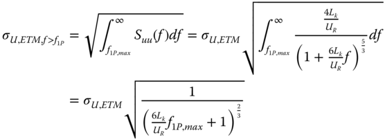
The turbulent wind speed encountered in normal operation in extreme turbulence conditions, which is used for cyclic/dynamic load analysis, is found by assuming normal distribution of the turbulent wind speed component. As opposed to the normal turbulence situations, the 95% confidence level value is taken. This is substituted into the quasi‐static equation used in Eq. ( 2.14). Equation (2.20) shows the expression for mudline moments.
Wind Scenario U‐3: Extreme Operating Gust (EOG) at Rated Wind Speed ( )
)
The maximum force is assumed to occur when the maximum mean thrust force acts and the 50‐year EOG hits the rotor. Due to this sudden gust, the wind speed is assumed to change so fast that the pitch control doesn't have time to adjust the blade pitch angles. This assumption is very conservative as the pitch control in reality has a time constant that would allow for some adjustment of the blade pitch.
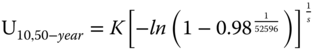
The methodology for the calculation of the magnitude of the 50‐year extreme gust is described in DNV (2014). This methodology builds on the long‐term distribution of 10‐minutes mean wind speeds at the site, which is typically represented by a Weibull distribution. The cumulative distribution function (CDF) can be written in the following form:
where K and s are the Weibull scale and shape parameters, respectively. From this the CDF of 1‐year wind speeds can be obtained using
where the number 52596 represents the number of 10‐minutes intervals in a year (52596 = 365.25[days/year]·24[hours/day]·6[10 min intervals/hour]).
From this, the 50‐year extreme wind speed, which is typically used in wind turbine design for extreme wind conditions, can be determined by the wind speed at which the CDF is 0.98 (i.e. 1‐year 10‐minutes mean wind speed that has 2% probability).
The extreme gust speed is then calculated at the rated wind speed from
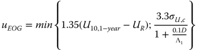
where D is the rotor diameter, Λ1 = Lk/8 with Lk being the integral length scale, σU, c = 0.11U10, 1 − year is the characteristic standard deviation of wind speed, U10, 1 − year = 0.8U10, 50 − year. Using this, the total wind load is estimated as
and using the water depth S and the hub height above sea level zhub, the mudline bending moment (without the load factor γL) is given as
Wind Scenario U‐4: Extreme Operating Gust (EOG) at the Cut‐Out Wind Speed (Uout)
This load case is examined here because intuitively it may seem natural to expect the highest loads when the turbine is operating at the highest operational wind speed, however, this is not the case. Wind load caused by the EOG at the highest operational wind speed (the cut‐out wind speed Uout) is calculated taking into consideration that the thrust coefficient expression of Frohboese and Schmuck (2010) is no longer valid. The thrust coefficient is determined from the assumption that the pitch control keeps the power constant. This means that the thrust force is inversely proportional to the wind speed above rated wind speed UR and the thrust coefficient is inversely proportional to the cube of the wind speed.
The EOG speed at cut‐out wind speed ![]() is determined as given (note that this differs for different mean wind speeds, i.e. the value is not the same at UR and at Uout). The thrust force and moment are then given by:
is determined as given (note that this differs for different mean wind speeds, i.e. the value is not the same at UR and at Uout). The thrust force and moment are then given by:
2.6.2.2 Spectral Density of Mudline Bending Moment
The spectral density of the turbulent thrust force on the rotor SFF, wind(f ) can be written as:

where D is the diameter of the rotor, Suu(f ) is the Kaimal spectrum, ![]() is the normalised Kaimal spectrum, ρa is the density of air, CT is the thrust coefficient, I is the turbulence intensity, and σU is the standard deviation of wind speed. The fore‐aft bending moment at the mudline is simply given by:
is the normalised Kaimal spectrum, ρa is the density of air, CT is the thrust coefficient, I is the turbulence intensity, and σU is the standard deviation of wind speed. The fore‐aft bending moment at the mudline is simply given by:
where H is the hub height above mean sea level and S is the mean sea depth (see Figure 2.6).
Similarly, the load can be reduced to any other cross section, such as the transition piece (TP). The mudline moment spectrum associated with wind speed fluctuations can be expressed as:
2.6.3 Wave Load
In simplified load calculation methodologies, to determine the wave loading, simple linear waves are assumed. Higher‐order theories like Stokes waves or Dean's stream function theory would provide better estimates, especially in shallow waters. However, the linear theory allows for simpler load calculation and its application is justified for foundation design loads.
A simplified approach to wave load estimation is Morison's (or MOJS) equation (Morison et al. 1950). In these equations, the diameter of the substructure is taken as DS = DP + 2tTP + 2tG[m] to account for the transition piece (TP) and the grout (tG) thickness. The circular substructure area AS is also calculated from this diameter. The methodology in this paper builds on linear (Airy) wave theory, which gives the surface elevation η, horizontal particle velocity w, and the horizontal particle acceleration ![]() as
as
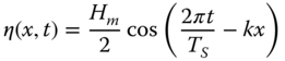
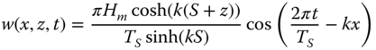
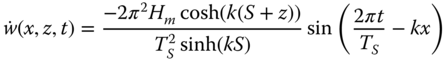
where x is the horizontal coordinate in the along‐wind direction (x = 0 at the turbine, see Figure 2.19) and the wave number k is obtained from the dispersion relation
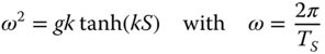
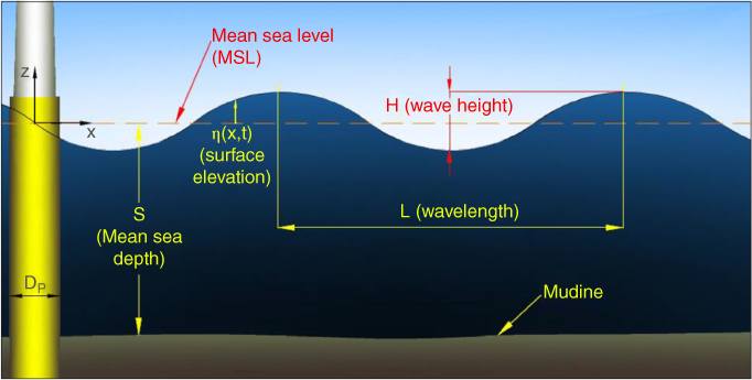
Figure 2.19 Definition of wave terminology.
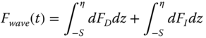
The force on a unit length strip of the substructure is the sum of the drag force FD and the inertia force FI:
where CD is the drag coefficient, Cm is the inertia coefficient, and ρw is the density of seawater. The total horizontal force and bending moment at the mudline is then given by integration as
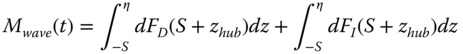
The peak load of the drag and inertia loads occur at different time instants, and therefore the maxima are evaluated separately. The maximum of the inertia load occurs at the time instant t = 0 when η = 0 and the maximum of the drag load occurs when t = TS/4 and η = Hm/2. The maximum load is then obtained by carrying out the integrations:
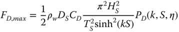
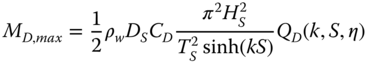
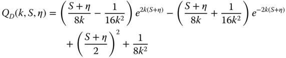
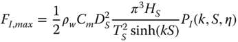
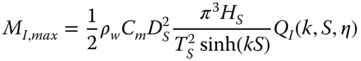

In the simplified method for obtaining foundation loads, it can be conservatively assumed that the sum of the maxima of drag and inertia loads is the design wave load. This assumption is conservative, because the maxima of the drag load and inertia load occur at different time instants. All wave scenarios (W‐1)–(W‐4) are evaluated with the same procedure, using different values of wave height H and wave period T.
2.6.4 1P Loading
A wind turbine is subjected to cyclic loading with the rotational frequency, and the source of this load is mainly the rotor mass imbalance and aerodynamic imbalance (due to differences in the pitch of individual blades). The amplitude of this forcing depends on the extent of the imbalances, and typical values can be used based on the literature. A simple method is shown to estimate the fore‐aft bending moment at the mudline caused by the mass imbalance; however, the calculation of the effect of blade pitch misalignment requires more input information and more sophisticated methods. The mass imbalance can be modelled as an added lumped mass on the rotor at θ azimuthal angle from Blade I. and at R distance from the centre of the hub, as shown in Figure 2.20. Here the imbalance is assumed to be on Blade I (θ = 0).
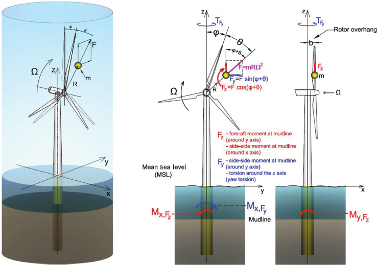
Figure 2.20 Model of the mass imbalance and loads exerted during operation. The fore‐aft mudline bending moment caused by the wind load and waves (assumed collinear) is  .
.
where Im is the mass imbalance with units of [kg·m], m is a lumped mass, and R is the radial distance from the centre of the hub along Blade I. The centrifugal force at any time can be calculated from the centrifugal acceleration a = RΩ2 with Ω being the angular frequency and f = Ω/(2π) the frequency of rotation. The lever arm of the centrifugal force Fcf is called the rotor overhang b (see Figure 2.20), with which the bending moment is expressed:
It is to be noted here that the centrifugal force also produces torsion in the tower (around the x‐axis), as well as moments in side‐to‐side direction (around the z‐axis), as shown in Figure 2.20. The bending moment in the side−side direction caused by the centrifugal force is much higher than the fore−aft moment because the arm of the force is H + MSL instead of b. The effect of the gravity force acting on the mass imbalance can be considered negligible.
2.6.5 Blade Passage Loads (2P/3P)
The wind produces drag force on the tower, which can be considered constant at a given mean wind speed, ignoring buffeting and vortex shedding on the tower and also without the effect of the rotating. When a blade passes in front of the tower, it disturbs the flow downwind and decreases the load on the tower. The frequency of this load loss is three times the rotational frequency of the turbine 3P (2P in case of two‐bladed designs). In a simplified method, the magnitude is estimated by a simple geometric consideration: the upper part of the face area of the tower is partly covered by the blade when the blade is in a downward pointing position (ϕ = π). The drag force on the covered part of the tower is taken to be zero and the blade causes a load loss on the tower. When the blade is in the downward direction, it covers the tower from z = H − L to z = H. The total moment of drag force on this upper section without the effect of blade passage:
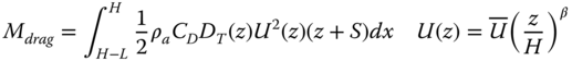
where H is the hub height from mean sea level, L is the length of the blades, ρa is the density of air, CD is the drag coefficient, D(z) is the diameter of the tower at z (assuming the diameter linearly decreases between the bottom and top diameters), z is the vertical coordinate (zero at mean sea level), S is the mean sea depth, and U(z) is the power law velocity profile using the exponential wind profile with β = 1/7 ≈ 0.143. If the ratio of the face area of the blade and the area of the top part of the tower (see Figure 2.16) is RA, then the 3P moment amplitude can be written:
2.6.6 Vertical (Deadweight) Load
The total vertical load on the foundation is calculated as
where m is the total mass of the structure
where mRNA is the total mass of the rotor‐nacelle assembly, mT = ρTDTπtTLT is the total weight of the tower, mTP = ρTP(DP + 2tG + tTP)πtTPLTP is the mass of the transition piece, and mP = ρPDPπtP(LP + LS) is the mass of the pile.
2.7 Order of Magnitude Calculations of Loads
The following sections discuss calculations for 1P loading, 3P loading, and typical values for wind and wave loading.
2.7.1 Application of Estimations of 1P Loading
To determine the 1P moment spectrum, one needs a typical value of the mass imbalance of the rotor. Some values are available for a somewhat smaller wind turbine studied in the literature. For the 2 MW Vestas V80 turbine, mass imbalance values of about 350–500 [kgm] were applied in these studies. The imbalance value is estimated for the 3.6 MW Siemens wind turbine by assuming that the imbalance is proportional to the mass of the rotor and also to the diameter of the turbine. The mass ratio and the diameter ratio of the rotors are calculated and the imbalance is scaled up by both ratios.
The mass of the rotor of the Vestas turbine is 37.5 tonnes, while that of the Siemens turbine is 95 tonnes. The diameter of the rotor of Vestas turbine is 80 m and that of the Siemens is 107 m. Therefore, the estimated imbalance value for the Siemens SWT‐107‐3.6 turbine is estimated as follows:

The original imbalance value of V80 is a value typical for an average operational wind turbine. As an upper bound estimate, one may consider Im = 2000 [kgm]. The distance between the axis of the tower and the centre of the hub (i.e. the rotor overhang) is estimated as b = 4 [m]. (For clarity, see Figure 2.20 for rotor overhang.) This way the maximum of the fore−aft bending moment caused by the imbalance can be written as:
The maximum bending moment occurs at the highest rotational speed of Ω = 13 [rpm], that is f = 0.2167 [Hz], its value is M1P = 0.015 [MNm].
Table 2.2 shows an example for this case study based on Arany et al. (2015a) and the readers are referred to this publication for further details.
Table 2.2 Moments due to 1P loads on the foundation.
| Mean wind speed at hub height |
Rotational speed Ω [rpm] | Fore−aft DAF [−] | 1P fore−aft mudline bending moment M1P[MNm]/(with DAF) | Side‐to‐side DAF [−] | 1P side‐to‐side mudline bending moment M1P, side − to − side[MNm]/(with DAF) |
| 5 | 5.8 | 1.09 | 0.002/(0.002) | 1.09 | 0.077/(0.084) |
| 9 | 9 | 1.25 | 0.007/(0.009) | 1.25 | 0.187/(0.234) |
| 15 | 13 | 1.71 | 0.015/(0.025) | 1.72 | 0.389/(0.669) |
| 20 | 13 | 1.71 | 0.015/(0.025) | 1.72 | 0.389/(0.669) |
The readers are also referred to Example 6.7 of Chapter 6and Arany et al. (2015a) for further details.
2.7.2 Calculation for 3P Loading
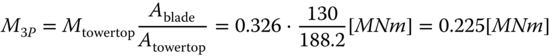
The 3P moment can be determined by estimating the total drag moment on the top part of the tower, which is covered by the downward‐pointing blade, and then reducing this moment by the ratio of the face area of the blade and the face area of the top part of the tower. The drag moment is estimated by the method presented in Section 2.3. The density of air is ρa = 1.225 [kg/m3], the drag coefficient of the tubular tower at high Reynolds number is CD ≈ 0.5 [−], and the linearly decreasing diameter of the tower can be written as:
with the z coordinate running from mean sea level along the length of the tower, Db and Dt are the bottom and top diameters of the tower, respectively. Using the exponential wind profile and the water depth S = 21.5 [m], the moment can be written as:

which gives Mdrag ≈ 0.326[MNm] for ![]() . Both the area of the blade and the area of the top part of the tower are approximated as trapezoids, the areas are calculated as:
. Both the area of the blade and the area of the top part of the tower are approximated as trapezoids, the areas are calculated as:

The magnitude of the load loss is then approximated as written in Eq. (2.45).
The drag load on the tower is calculated by integrating along the whole tower:

The 3P forces and moments are estimated in Table 2.3 for several values of the mean wind speed. Note that in the vicinity of 6.125 m s−1 (∼6.7 rpm rotational speed), the DAF gets very high and the 3P moment is an order of magnitude higher than without DAF.
Table 2.3 3P loading and drag load on the tower.
| Wind speed |
Total drag force on the tower [MN] | Total drag moment on the tower [MNm] | 3P freq. [Hz] | DAF [−] | 3P force F3P[MN]/(with DAF) | 3P moment M3P[MNm]/(with DAF) |
| 5 | 0.0019 | 0.176 | 0.29 | 3.77 | 0.001/(0.003) | 0.069/(0.262) |
| 9 | 0.0062 | 0.570 | 0.45 | 1.23 | 0.003/(0.004 | 0.225/(0.275) |
| 15 | 0.0173 | 1.584 | 0.65 | 0.36 | 0.008/(0.003) | 0.625/(0.225) |
| 20 | 0.0308 | 2.816 | 0.65 | 0.36 | 0.014/(0.005) | 1.111/(0.401) |
| 6.125 (resonance) | 0.0289 | 0.189 | 0.335 | 10 | 0.001/(0.013) | 0.104/(1.042) |
2.7.3 Typical Moment on a Monopile Foundation for Different‐Rated Power Turbines
Based on the method described in the chapter and developed in Arany et al. (2015a,b, 2017), Table 2.4 shows typical values of thrust due to the wind load acting at the hub level for five turbines ranging from 3.6 to 8 MW. The thrust load depends on the rotor diameter, wind speed, controlling mechanism, and turbulence at the site. The mean and maximum mudline bending moment on a monopile is also listed. Wave loads strongly depend on the pile diameter and the water depth and it is therefore difficult to provide a general value. Table 2.4 contains a relatively severe case of 30 m water depth and a maximum wave height of 12 m.
Table 2.4 Typical wind and wave loads for various turbine sizes for a water depth of 30 m.
| Turbine rated power | ||||||
| Parameter | Unit | 3.6 MW | 3.6 MW | 5.0 MW | 6–7 MW | 8 MW |
| Rotor diameter | m | 107 | 120 | 126 | 154 | 164 |
| Rated wind speed | m s−1 | 13 | 13 | 11.4 | 13 | 13 |
| Hub height | m | 75 | 80 | 85 | 100 | 110 |
| Mean thrust at hub (from wind) | MN | 0.50 | 0.60 | 0.60 | 1.00 | 1.20 |
| Max thrust at hub (from wind) | MN | 1.00 | 1.20 | 1.20 | 2.00 | 2.30 |
| Mean mudline moment from wave Mmean | MNm | 53 | 69 | 70 | 135 | 165 |
| Max mudline moment from wave Mmax | MNm | 103 | 136 | 137 | 265 | 323 |
| Water depth | m | 30 | 30 | 30 | 30 | 30 |
| Maximum wave height | m | 12 | 12 | 12 | 12 | 12 |
| Typical monopile diameter | m | 5.5 | 6 | 6.5 | 7 | 7.5 |
| Horizontal wave force | MN | 3.67 | 4.2 | 4.8 | 5.43 | 6.1 |
| Mudline moment from waves | MNm | 104 | 120 | 137 | 155 | 175 |
| Unfactored design moment (wind+wave) | MNm | 207 | 256 | 274 | 420 | 498 |
Typical values of wave loading ranges between 2 and 10 MN acting at about three‐fourths of the water depth above the mudline, which must be added to the wind thrust. Typical peak wave periods are around 10 seconds. The pattern of overturning moment on the monopile is schematically visualised in Figure 2.21. In the figure, a typical value of the peak period of wind turbulence is taken and can be obtained from wind spectrum data.
Note. It may be noted that only wind and wave moments are considered in the Figure 2.21. 1P and 3P moments are ignored, as they are about three orders of magnitude lower.
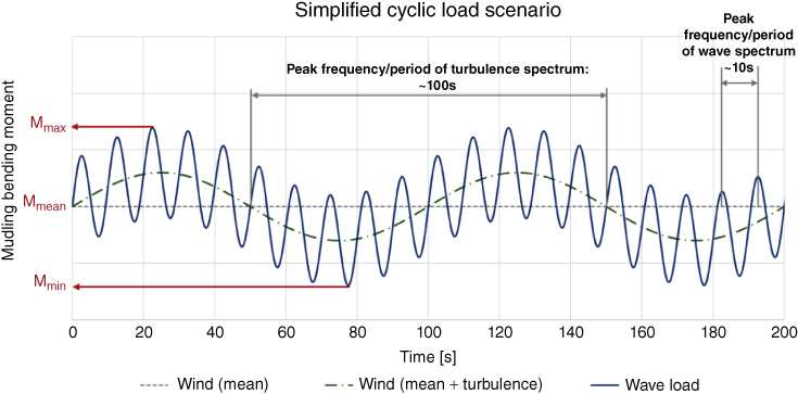
Figure 2.21 Mudline moment due to wind and wave load, wind and waves collinear.
2.8 Target Natural Frequency for Heavier and Higher‐Rated Turbines
Figure 2.22 shows a 1P range frequency plots for different turbines ranging from 2 to 8 MW. It is clear that as the turbine size/rated power increases, the target frequency in a soft‐stiff design is moving towards the left of the spectrum. For example, the target frequency of a 3 MW turbine is in the range of 0.35 Hz. In contrast, the target frequency for an 8 MW turbine is 0.22–0.24 Hz, which can be very close to wave frequencies. This can also be explained through a Campbell diagram plotted in Figure 2.23, which shows the narrow band of the target frequency for an 8 MW turbine.
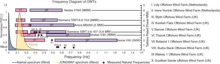
Figure 2.22 Importance of dynamics with deeper offshore and larger turbines.
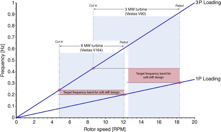
Figure 2.23 Campbell diagram for a 3 and 8 MW turbine.
2.9 Current Loads
Current loads act on the substructure due to the horizontal movement of water particles causing drag. Several effects may be the source of ocean currents and the most important from the point of view of OWT foundations are wind‐induced currents and tidal currents. An approach to model currents is to choose a velocity profile, along the water depth and apply it to the substructure. Generally speaking, the velocity of current in the upper regions are driven by wind and in deeper down by tidal and other effects. The velocity typically reduces to zero at the seabed.
Since current speeds are subjected to high levels of uncertainty, a conservative approach to current load modelling is to assume a constant current velocity along the depth. The velocity may be assumed to be the maximum value expected in 50 years and may be taken as 1% of the 50‐year extreme mean wind speed. Using the constant profile, the load due to current can be estimated similar to the drag load acting on the substructure.
2.10 Other Loads
There are other loads that need to considered while designing a wind farm and are listed below:
- Ice loads on the blades
- Floating ice sheet impact loads on the substructure
- Ship impact loads on the substructure
- Loads due to installation errors and residual stresses on the foundation
- Start‐up loads and emergency shut‐down loads
- Earthquake and tsunami loads
- Emergency fault case loads
Specialist literature and codes are recommended for further reading. Only earthquake and tsunami loads are discussed here.
2.11 Earthquake Loads
Many of the potential offshore wind farm locations are seismically active and therefore require proper analysis to safeguard investments. Wind energy production from offshore wind farms is a reality nowadays around the world. Figure 2.24 shows the main countries that are developing and investing in offshore wind power according to the Global Wind Energy Council following De Risi et al. (2018). In the same figure is shown a global seismic hazard map in terms of peak ground acceleration (PGA) with probability of exceedance of 10% in 50 years based on GSHAP model. Several countries are in high seismic regions, including the United States, China, India, and South‐East Asia, and are also adjacent to subduction zones shown by blue lines. In these zones magnitude M9‐class megathrust earthquakes can potentially occur.
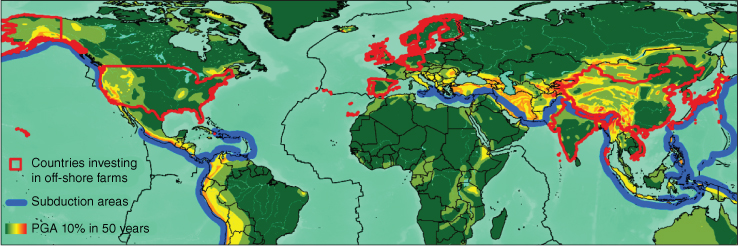
Figure 2.24 Map of countries investing in offshore wind farms (red boundaries), subduction trenches (blue lines), and global seismic hazard map, see De Risi et al. (2018).
Figure 2.25 shows normalised spectra for typical wind, sea wave, and ground shaking and on the same figure range of periods for the first vibration modes and higher modes are also superimposed. It is possible to observe that the first modes usually fall in the range of periods where the spectral content of earthquake ground motions are in decay but are still relatively high, and this depends on the characteristics of earthquake scenarios and local site conditions. Therefore, it is essential to understand which seismic events and soil conditions may excite such periods and if higher modes play significant role in the seismic behaviour.
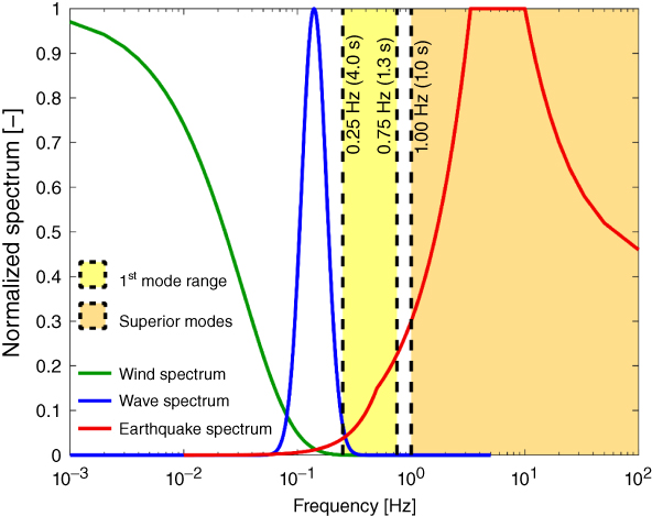
Figure 2.25 Typical normalised spectra of actions due to wind, sea waves, and earthquake ground motions. The yellow and orange bands represent the ranges of vibration periods for conventional wind turbines corresponding to main and higher modes, respectively, in De Risi et al. (2018).
Design of OWT structures in seismic regions involves following steps:
- A detailed seismic hazard analysis (SHA) must be conducted. One of the important outcomes will be PGA expected at the site during its design life in deterministic and probabilistic format.
- Identification of potential seismic hazards at the site. This must also include cascading events. Examples are:
- Effect of large fault movements.
- Shaking with no‐liquefaction of the subsurface. This includes inertial effects on the structure and inertial bending moment on the foundation piles.
- Shaking + Liquefaction of the subsurface. Liquefaction may lead to a large, unsupported length of the pile and elongate the natural vibration period of the whole structure. The ground may liquefy very quickly or may take time and is a function of ground profile and type of input motion. In such scenarios, the transient effects of liquefaction need to be considered, as it will affect the bending moment in the piles.
- Shaking + Liquefaction + Tsunami.
- Shaking + Landslide.
- Earthquake sequence such as: Foreshock + Mainshock + Aftershock.
- Generation of input motion for the site depends on the seismo‐tectonics of the area. This includes faulting pattern, distance of the site from earthquake source, wave travelling path, geology of the area, etc. This can be either synthetic (artificially generated) or recorded ground motion from previous earthquakes.
- Site response analysis is how the ground will behave under the action of the input motion.
- Dynamic SSI analysis incorporates the knowledge of the site response into the calculations.
2.11.1 Seismic Hazard Analysis (SHA)
A detailed SSA can be divided into three parts: (i) Estimation of seismic hazard by carrying out deterministic seismic hazard analysis (DSHA) and probabilistic seismic hazard analysis (PSHA); (ii) evaluation of local site effects by carrying out nonlinear ground response analysis; and (iii) preparation of hazards maps and response spectra.
Two approaches, probabilistic (PSHA) and deterministic (DSHA), are commonly adopted for seismic hazard assessment. In DSHA, a particular earthquake scenario is assumed based on earthquake data and tectonic setup of the study area. The hazard is estimated on the basis of attenuation characteristics of the region. For a worst‐case scenario, DSHA is more useful. Hazard is evaluated considering the closest distance between the source and the site of interest as well as the maximum magnitude for the fault.
To evaluate seismic hazard deterministically for a particular site or region, all possible sources of seismic activity are identified and their potential for generating strong ground motion is evaluated. It is used widely for nuclear power plants, large dams, large bridges, hazardous waste containment facilities, and also as a ‘cap’ for PSHA. On the contrary, in probabilistic method (PSHA), the uncertainties in earthquake size, location, and time of occurrence are explicitly considered, see Figure 2.26 for the steps.
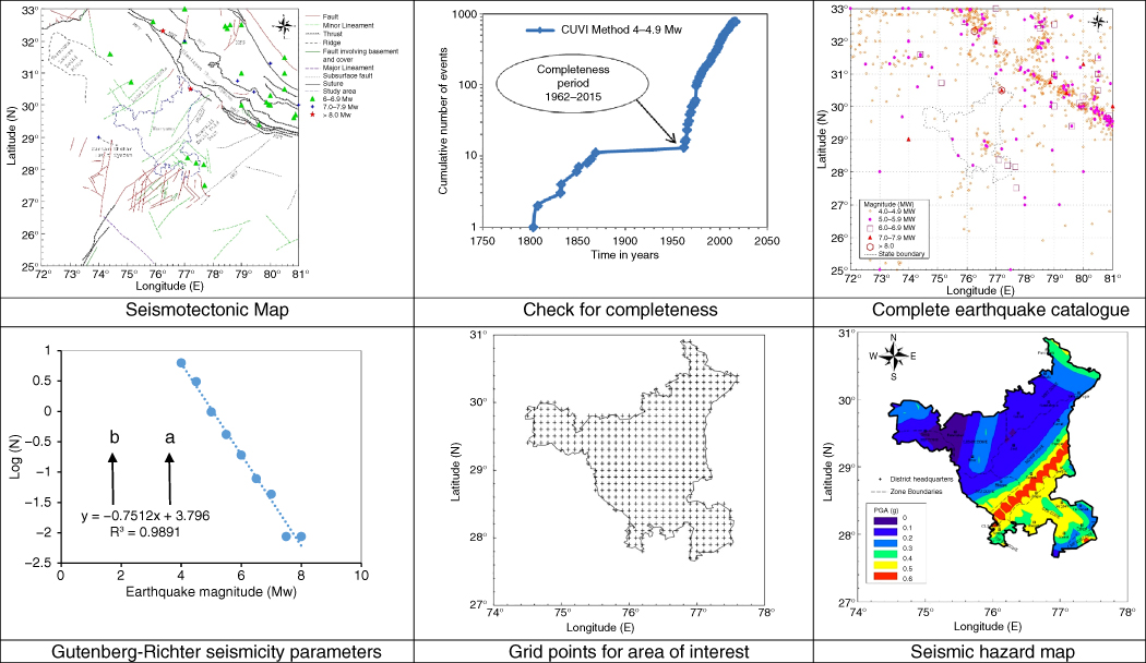
Figure 2.26 Steps in PSHA. [Courtesy: Nitish Puri].
The procedure followed in carrying out the SHA is as follows:
- Consider an area covering 300–500 km radius around point of interest as seismic study area.
- Collect all the tectonic information such as location, magnitude, and depth of earthquakes occurred, and satellite imageries of the fault lines for the seismic study area.
- All this information has to be merged to prepare a single map (seismotectonic map), which represents tectonic setting of the seismic study area.
- Prepare an earthquake catalogue for the study region, which includes all recordings from pre‐instrumental and instrumental period. Try to collect data from all the possible sources. Check the catalogue for duplicity of events, clustering of events, and completeness.
- Determine Gutenberg‐Richter seismicity parameters a and b for the estimation of rate of occurrence of different magnitudes of earthquake and return periods. For DSHA, this step can be avoided.
- Identify the tectonic features likely to generate significant ground motions in the study area. Also assign maximum observed magnitude (Mobs) to each source.
- Calculate the maximum magnitude potential (Mmax) for all the seismogenic sources present in the study area. For PSHA, it is important to consider uncertainty in size of earthquake.
- Consider a suitable grid on the area of interest for e.g. 0.2° × 0.2° for a country, 0.1° × 0.1° for a state, and 0.005° × 0.005° for a city.
- Compute shortest distance of grid points to each seismogenic source. For PSHA, it is important to consider uncertainty in the location of earthquake.
- Select a suitable ground motion prediction equation (GMPE), which accurately represents the tectonic setup of the study area. In case of nonavailability of regional GMPEs, GMPEs developed for other regions can also be used, provided their source and site characteristics are similar to the study area. For PSHA, it is necessary to handle epistemic uncertainty in the GMPEs. This can be handled by adopting logic tree approach.
- For the computation of hazard at a grid point, compute ground motion parameters with respect to various seismogenic sources and identify the source causing maximum ground motion at the point of interest. For that grid point, consider the maximum magnitude potential of that seismogenic source as the controlling earthquake.
- Site amplification factors can be estimated by carrying out linear, equivalent linear, or nonlinear ground response analysis.
2.11.2 Criteria for Selection of Earthquake Records
Ground motion records to be used in analysis should represent the potential earthquake hazards at the site i.e. consideration of magnitude, distance, site conditions, source mechanism, directivity, and other effects obtained from SSA. In this regard, the appendix of ISO 19901‐2 states that a minimum of four records should be used for analysis, and that each record should be selected according to the following criteria:
Given the magnitude and distance of events dominating extreme level earthquake (ELE) ground motions, the earthquake records for time history analysis can be selected from a catalogue of historical events. Each earthquake record consists of three sets of tri‐axial time histories representing two orthogonal horizontal components and one vertical component of motion. In selecting earthquake records, the tectonic setting (e.g. faulting style) and the site conditions (e.g. hardness of underlying rock) of the historical records should be matched with those of the structure's site.
Three approaches are often used, and all these methods have their advantages and disadvantages and are discussed later in this section through an example.
2.11.2.1 Method 1: Direct Use of Strong Motion Record
In this method, a strong motion is chosen to match the seismicity of the place, either in terms of moment magnitude or expected peak bed rock acceleration (PBRA) also known as PGA. It may be difficult to find a recorded motion satisfying both the requirements. For example, a site may expect a magnitude 6.0 earthquake and a PBRA of 0.2 g. Therefore, a designer has to look for the recorded data matching these characteristics. This method is rarely used in practice, as it is quite unlikely that the shape of the spectra will match the expected bedrock spectra at a particular site. This will be illustrated later using an example.
2.11.2.2 Method 2: Scaling of Strong Motion Record to Expected Peak Bedrock Acceleration
In this method, an earthquake record is chosen from a database to match the moment magnitude and then the maximum amplitude is scaled to match the expected PBRA.
2.11.2.3 Method 3: Intelligent Scaling or Code Specified Spectrum Compatible Motion
Traditionally, seismic hazard at a site for design purposes has been represented by design spectra. Thus, all seismic design codes and guidelines require scaling of selected ground motion time histories so that they match or exceed the controlling design spectrum within a period range of interest. Figure 2.27 shows the response spectra of IS: 1893 (2002) for hard soil or rock together with a Chi‐Chi (Taiwan) earthquake motion and spectrally matched motion. Several methods of scaling time histories are available that involve rigorous mathematics.
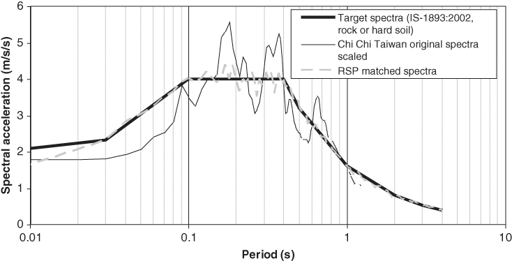
Figure 2.27 An example of earthquake spectra of selected motion matched to code‐specified spectra.
Essentially, in all these methods, an input motion is selected from a strong motion database, and the motion is manipulated in such a way so as to obtain a motion that matches the target design spectra. The manipulation can be carried out in frequency‐domain where the time‐frequency content of the recorded ground motions is manipulated in order to obtain a good match. Mathematically, this can be expressed as follows, following Alexander et al. (2014): a process that can transform a known signal or input motion x(t) into a similar input motion y(t) that matches the spectrum. The additional aim is that transformed signal y(t) should maintain very similar nonstationary characteristics such as general envelope, time location of large pulses, and variation of frequency content with time. In other words, the aim signal y(t) should look, for all intents and purposes, like a real earthquake.
Figure 2.28 shows the response spectra for different types of earthquake that can also be used to estimate the inertia forces on the structure. For example, for a three‐second period wind turbine structure, the spectral acceleration will be function of the location and can be read off the ordinate (y‐axis).
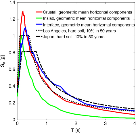
Figure 2.28 Response spectra for different types of earthquakes.
2.11.3 Site Response Analysis (SRA)
Once the bedrock motion is obtained, the vertically propagating shear waves are convoluted through the soil depth using a SRA to obtain the site effects. Figure 2.29 shows a schematic diagram of the methodology. Various software exist in performing this particular function such as SHAKE 91, DEEPSOIL, DMOD, EERA, Cyclic 1D. For liquefiable deposits, Cyclic 1D can be used to perform the SRA, as it uses an advanced constitutive model for the liquefied soil developed by Parra (1996) and Yang (1999) in its analysis. Literature can be found on the use of various site response analysis programs, which capture various nonlinear aspects of the soil in Hashash et al. (2010).
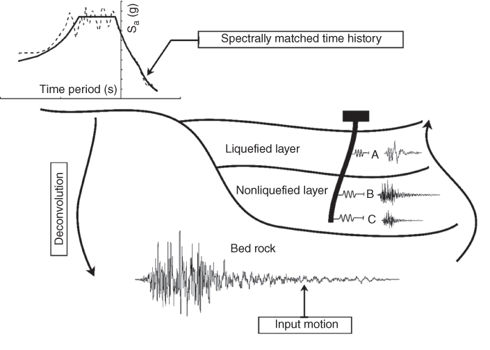
Figure 2.29 Schematic of ground response analysis.
2.11.4 Liquefaction
Apart from site response analysis, it is necessary to predict if the subsurface will liquefy. The part of the foundation in liquefiable soil needs to be considered as laterally unsupported. Therefore, the length of the tower will effectively increase leading to elongation of natural period. From the point of analysis, liquefaction may be assumed to progress along the depth of the soil layer in top‐down fashion. A modal analysis can be carried out to study the variation of depth of liquefaction (DL) with the first natural period of the soil‐pile system. The results are plotted in Figure 2.30, which is a graphical representation of normalised elongation of period for various depths of liquefaction. In Figure 2.30, DL represents depth of liquefaction, L is the embedded length of the pile, T is the time period, and Tinitial is the initial time period of the structure. However, this is momentary, and as the earthquake stops, the ground resolidifies and most of the ground stiffness is regained. Three cases are considered in the study:
- Post liquefaction, the American Petroleum Institute (API) prescribed soil spring stiffness is degraded 92% using a p‐multiplier as per Brandenberg (2005).
- Zero initial stiffness and strength are provided to the p‐y spring for the liquefied soil as per RTRI (1999).
- Hyperelastic p‐y spring for liquefiable soils (Lombardi et al. (2017).
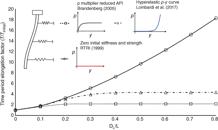
Figure 2.30 Elongation of a period of a pile due to different liquefiable depths for a given pile geometry and ground profile.
As the eigenvalue analysis is linear, only the initial stiffness of the p‐y curves (reduced API, hyperelasticity, zero strength API) is used in the model to compute the natural frequencies of the soil‐pile system.
2.11.5 Analysis of the Foundation
Analysis of foundations is usually carried out using beams on nonlinear Winkler foundation approach as shown in Figure 2.31. Various details of modelling are discussed in Dash et al. (2010). Once the DL is estimated, it is important to use the Winkler or p‐y springs of appropriate shape as shown in the figure. The shape of non‐liquefied and liquefied p‐y curves are very different. The seismic forces, HPre (pre‐liquefaction) and HPost (post‐liquefaction), depend on the time period of the whole structure and can be estimated based on the response spectra of the site.
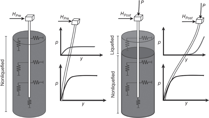
Figure 2.31 Beam on nonlinear winkler model.
The aim of this section is to further the discussion carried out in Section 1.1 of Chapter 1 on the good performance of a near‐shore wind farm. Calculations were carried out based on the available information of the ground profile and the turbine characteristics. In the absence of data, engineering judgements were used to carry out the analysis in order to draw broad conclusions. The focus of the investigation is the behaviour during the 2011 Tohoku earthquake seismic shaking and during the tsunami run‐up, discussed in the following examples.
2.12 Chapter Summary and Learning Points
- One of the first step in design of foundation is to fix the target frequency. To visualise the ‘target frequency’ it is necessary to construct the spectrum of the frequencies acting on the wind turbine structure, and this requires understating of wind and wave loading. The method proposed to visualise the target frequency is given in Figures 2.4 and 2.5, and it may be noted that the magnitudes of the spectral densities are normalised to 1. In reality, wind and wave will have few orders of magnitude higher energy than 1P and 3P. Order of magnitude calculations are shown in the chapter for some case studies.
- The motivation behind PSD formulation of the bending moment for the different loads is to provide a basis for a quick frequency domain fatigue damage estimation. This is particularly useful in the preliminary design phase of these structures, which is otherwise a very lengthy process and is usually done in time domain. This would also encourage integrated design of OWTs incorporating the dynamics and fatigue analysis in the early stages of structural design. Examples of frequency domain methods are the Dirlik, Tovo‐Benasciutti, α0.75 methods.
- The formulations and methods presented had an objective to use the minimum information possible to obtain the loads such that simple spreadsheet‐based methods can be used to estimate the loads. Information such as the control parameters, the blade design, aerofoil characteristics, and generator characteristics are not included in this formulation. These can be carried out in aero‐hydro‐servo‐elastic analysis such as HAWC, FAST, BLADED.
- For soft‐stiff design, where the target frequency is placed between upper bound of 1P and lower bound of 3P, any change in natural frequency will enhance the dynamic amplifications, which will increase the vibration amplitudes and thus the stresses and fatigue damage on the structure.