CHAPTER 6
Measuring the Costs of Environmental Protection
6.0 Introduction
When the Environmental Protection Agency (EPA) tightened the national air-quality standard for smog (ground-level ozone), the agency developed official cost estimates for this regulation, ranging from $600 million to $2.5 billion per year. Where do numbers such as this come from?1
On the face of it, measuring the costs associated with environmental cleanup appears substantially easier than measuring the benefits. One can simply add up all the expected expenditures by firms on pollution-control equipment and personnel, plus local, state, and federal government expenditures on regulatory efforts, including the drafting, monitoring, and enforcing of regulations. This engineering approach to measuring cost is by far the most widespread method in use.
However, because engineering cost estimates are often predicted costs, they require making assumptions about future behavior. For example, cost estimates may assume full compliance with pollution laws or assume that firms will adopt a particular type of pollution-control technology to meet the standards. To the extent that these assumptions fail to accurately foresee the future, engineering cost estimates may be misleading on their own terms. In a famous case of getting it wrong, the EPA overestimated the costs of sulfur dioxide control by a factor of two to four; “credible” industry estimates were eight times too high.2
Moreover, from the economic point of view, there are additional problems with the engineering approach. Economists employ a measure of cost known as opportunity cost: the value of resources in their next best available use. Suppose that the new smog laws lead to engineering costs of $2 billion per year. If, as a society, we were not devoting this $2 billion to pollution control, would we be able to afford just $2 billion in other goods and services? More? Less? The answer to this question provides the true measure of the cost of environmental protection.
Engineering cost estimates will overstate the true social costs to the extent that government involvement (1) increases productivity by increasing the efficiency with which available resources are used, forcing technological change or improving worker health or ecosystem services, and/or (2) reduces unemployment by creating “green jobs.”
On the other hand, engineering cost estimates underestimate the true social costs to the extent that government involvement (1) lowers productivity growth by diverting the investment and/or (2) induces structural unemployment. This chapter first examines the EPA estimates of economy-wide engineering costs, along with an example of the potential costs of reducing global warming pollution. We then consider the degree to which these estimates overstate or understate the “true” costs of environmental protection. We end with a final look at benefit–cost analysis and its role in generating more efficient environmental protection.
6.1 Engineering Costs
Engineering cost estimates require the use of accounting conventions to “annualize” capital investments—in other words, to spread out the cost of investments in plant and equipment over their expected lifetimes. Table 6.1 provides EPA estimates of the historical “annualized” engineering costs of pollution control in the United States since the major federal programs were initiated in the early 1970s through to the year 2000.
TABLE 6.1 U.S. Annualized Pollution-Control Costs (2005 $ billion)
Source: Carlin (1990).
| Year | ||||
| Type of Pollutant | 1972 | 1980 | 1990 | 2000 |
| AIR | ||||
| Air | $12.9 | $28.8 | $45.1 | $71.5 |
| Radiation | $0.0 | $0.2 | $0.7 | $1.5 |
| WATER | ||||
| Quality | $14.9 | $37.3 | $63.5 | $93.4 |
| Drinking | $1.3 | $3.2 | $5.6 | $10.7 |
| LAND | ||||
| Waste disp. | $13.7 | $22.2 | $40.5 | $61.9 |
| Superfund | $0.0 | $0.0 | $2.8 | $13.1 |
| CHEMICALS | ||||
| Toxics | $0.1 | $0.7 | $0.9 | $2.0 |
| Pesticides | $0.1 | $0.8 | $1.6 | $2.8 |
| OTHER | $0.1 | $1.5 | $2.7 | $3.7 |
| TOTAL | $43.3 | $94.6 | $163.6 | $260.3 |
| % of GNP | 0.9 | 1.6 | 2.1 | 2.8 |
Note: Both the costs and GNP shares from 1990 to 2000 are estimated.
The table lists the historical annual pollution-control expenditures for four categories of pollutants—air, water, land, and chemicals—as well as an “other” category including unassigned EPA administrative and research expenses. The costs listed cover all direct compliance and regulatory expenses for pollution control, including investments in pollution-control equipment and personnel, the construction of municipal water treatment plants, and the bill your family pays to your local garbage collector. (Note that these costs are not identical to the costs of environmental regulation: even without regulations, the private sector would undertake some level of sewage treatment and garbage disposal!)
As a nation, we are indeed devoting greater attention to pollution control. Over a period of 25 years, total spending rose from $43 billion to more than $260 billion. Perhaps, more significantly, pollution control as a percentage of GNP rose from less than 1 percent in 1972 to 2.1 percent in 1990 to more than 2.8 percent by 2000. Thus, pollution control more than doubled its claim on the nation’s resources.
The next big step in pollution control for the United States, and the rest of the world, is attacking global warming. Figure 6.1 provides one engineering-cost assessment of reducing global warming emissions in the United States. On the vertical axis, the figure shows the marginal costs in $ per metric ton of e ( “equivalents” or plus other greenhouse gases) reduced from a variety of measures and technologies that are already available today. On the horizontal axis, the figure illustrates the total reduction in millions of metric tons of e per year achieved by taking these steps. The graph illustrates the steps that together could reduce emissions in total by 600 million tons if phased in by 2030—about 10 percent of current U.S. emissions.

FIGURE 6.1 Marginal Cost of Reduction Curve for U.S. CO2e, Beyond Business-as-Usual, 2030
Source: Adopted from King County (2015: 30).
First note that the researchers argue that the first 250 million tons can actually be obtained at a negative cost. These measures would actually save businesses and households money. For example, the very first bar is labeled “residential lighting.” Much of the cost and emissions savings here come from switching to LED (light-emitting diode) sources, which use about half the energy of compact fluorescent (CFL) bulbs and about one-tenth that of a conventional incandescent lamp. Making the switch to LED and other more efficient lighting options would save consumers $90 in reduced energy costs for every ton of emissions reduced. Total cost savings from improved lighting would be the area of the box: $90 × 12 million tons, or $108 million a year.
Close to the zero dollar point are improvements in power plant efficiency (savings of about $15 per ton) and increased residential insulation (costs of $5 per ton). Finally, at the high end in this technology list is biomass co-firing of coal-fired power plants, that is, burning wood or other renewable biomass mixed with coal, thereby reducing net CO2 emissions. This is estimated to cost around $30 per ton of CO2 reduced.
A quick puzzle: How would you calculate the total cost of reducing 600 million tons from the data in the marginal cost curve in Figure 6.1? You can eyeball from the graph that the cost savings represented by the boxes seem to be a bit greater than the increased expenditures. (See Application 6.1 for more details.) If you add up the savings plus the costs, the answer is a small net savings—in other words, this estimate argues that the United States could get the first 10 percent of reductions in emissions and, on net, make some money in doing so.
A similar “bottom up” exercise based on evaluating various technology solutions estimated the annual global costs for reducing emissions to stabilize the climate at a 4 degrees F increase, the UN’s target to limit warming.3 This would require much deeper cuts than those shown in Figure 6.1. The figure came out to be a cost of around 1 percent of global GDP—currently about $500 billion. So, if the United States does aggressively attack global warming, then over time, the annual engineering costs of pollution control might rise by 1 percent point, from around 3 percent of U.S. GDP to about 4 percent. The question we seek to answer in the rest of the chapter is this: Do these engineering estimates understate or overstate the true social costs of environmental protection?
6.2 Productivity Impacts of Regulation
Undoubtedly, the biggest unknown when it comes to estimating the costs of environmental protection is its impact on productivity. Productivity, or output per worker, is a critical economic measure. Rising productivity means that the economic pie per worker is growing. A growing pie, in turn, makes it easier for society to accommodate both the needs of a growing population and the desire for a higher material standard of living.
Between 1974 and 1995, productivity growth in the United States averaged only 1 percent, well below the 3 percent rate the American economy experienced in the 1950s and 1960s. And because growth is a cumulative process, the small changes in productivity had dramatic long-run effects. If, rather than declining after 1974, productivity growth had continued at its 1950 to 1970 rate of 3 percent, GDP in 2007 would have been several trillion dollars greater than it actually was!
Although productivity growth rebounded after 1995, some have charged that environmental regulations specifically were a major contributor to the productivity slowdown. By contrast, others have argued that pollution-control efforts can spur productivity growth by forcing firms to become more efficient in their use of resources and adopt new and cheaper production techniques. As we will see, this debate is far from settled. But, because productivity growth compounds over time, the impact of regulations on productivity—whether positive or negative—is a critical factor in determining the “true” costs of environmental protection.
First, let us evaluate the pro-regulation arguments. Theoretically, regulation can improve productivity in three ways: (1) by improving the short-run efficiency of resource use; (2) by encouraging firms to invest more or invest “smarter” in the long run; and (3) by reducing health-care or firm-level cleanup costs, which then frees up capital for long-run investment.
You can clearly see an example of the short-run efficiency argument in Figure 6.1. The economists who estimated the cost curve for attacking global warming pollution believe they have identified hundreds of billions of dollars of waste in the global economic system. Tremendous cost savings could be immediately achieved, if firms (and households) would only adopt the already existing, energy-efficient technologies—more efficient lighting, cooling, heating, and mechanical systems. These savings in turn would free up capital for productive investment in other sectors of the economy. However, other economists are suspicious that these so-called free lunches are actually widespread, arguing on theoretical grounds that “there ain’t no such thing.” Why would competitive firms ignore these huge cost-saving opportunities if they really existed? Chapter 19 is devoted to a discussion of energy policy and the free-lunch argument. For now, recognize that should it be the case that regulation forces firms to use energy more cost-effectively, greater output from fewer inputs, and thus an increase in productivity, will result.
The second avenue by which regulation may increase productivity is by speeding up, or otherwise improving, the capital investment process. The so-called Porter hypothesis, named after Harvard Business School Professor Michael Porter, argues that regulation, while imposing short-run costs on firms, often enhances their long-run competitiveness.4 This can happen if regulation favors forward-looking firms, anticipates trends, speeds investment in modern production processes, encourages R&D, or promotes “outside the box,” nonconventional thinking.
For example, rather than installing “end-of-the-pipe” equipment to treat their emissions, some firms have developed new production methods to aggressively reduce waste, simultaneously cutting both costs and pollution. In this case, regulation has played a technology-forcing role, encouraging firms to develop more productive manufacturing methods by setting standards they must achieve. More broadly, as was discussed in Chapter 3, the whole sustainable business movement is predicated on solving environmental problems, profitably, and achieving superior business performance by reducing risks, improving resource efficiency, and developing innovative substitutes for polluting products and processes. A number of studies have supported the Porter hypothesis, finding that firms known for environmental leadership are no less profitable, and often are more profitable than the average in their industry.5
Finally, the third positive impact of regulation on productivity is from the health and ecosystem benefits that arise from environmental protection. In the absence of pollution-control measures, the U.S. population would have experienced considerably higher rates of sickness and premature mortality. In addition, firms that rely on clean water or air for production processes would have faced their own internal cleanup costs. These factors would have reduced productivity directly and also indirectly because expenditures on health care and private cleanup would have risen dramatically. This spending, in turn, would have represented a drain on productive investment resources quite comparable to mandated expenditures on pollution control.
Productivity may also be dampened in a variety of ways. First, regulation imposes direct costs on regulated firms; these costs may crowd out investment in conventional capital. Second, a further slowdown in new investment may occur when regulation is more stringent for new sources of pollution, as it often is. Third, regulation will cause higher prices for important economy-wide inputs such as energy and waste disposal. These cost increases, in turn, will lead to reductions in capital investment in secondary industries directly unaffected by regulation, for example, the health and financial sectors of the economy.
Finally, regulation may frustrate entrepreneurial activity. Businesspeople often complain about the “regulatory burden” and “red tape” associated with regulation, including environmental regulation. Filling out forms, obtaining permits, and holding public hearings all an additional “hassle” to business that may discourage some investment.
However, despite the chorus of voices attacking regulation as one of the main culprits in explaining low levels of American productivity growth, evidence for this position is not strong. On balance, federal environmental regulations primarily put in place in the 1970s and 1980s somewhat reduced the measured productivity in heavily regulated industries; yet, such effects account for only a small portion of the total productivity slowdown. Moreover, in the absence of regulation, productivity would have fallen anyway due to increased illness and the subsequent diversion of investment resources into the health-care field. Finally, there is scattered evidence for productivity improvements arising from regulation, following both the Porter hypothesis and the energy-efficiency lines of argument. Rolling back environmental laws to their 1970 status, even if this were possible, would at best make a small dent in the problem of reduced U.S. productivity and might easily make things worse.6
Nevertheless, due to the large cumulative effects on the output of even small reductions in productivity growth, minimizing the potential negative productivity impacts is one of the most important aspects of sensibly designed regulatory policy. As we shall see in Chapters 15 and 16, regulations can be structured to better encourage the introduction of more productive, and lower cost, pollution-control technologies. Bottom line: long-run productivity impacts are important, and economy-wide, it is difficult to assess their overall impact—either in direction or in magnitude. Thus, the true cost of existing or proposed environmental cleanup measures can be difficult to assess—yet another challenge to benefit–cost-based decision-making.
6.3 Employment Impacts of Regulation
Is environmental protection (1) a “job killer,” (2) a “green jobs” engine, or (3) neither of these? Many people do believe there may, in fact, be a serious jobs versus environment trade-off. In one poll, an astounding one-third of respondents thought that somewhat or very likely their own jobs were threatened by environmental regulation!7
Much of this perception is due to overheated political rhetoric. A case in point was that of the 1990 Clean Air Act Amendments, which regulated both sulfur dioxide emissions from acid rain and airborne toxic emissions from factories. In the run-up to the legislation, economists employed by industry groups predicted short-term job losses, ranging from “at a minimum” of 200,000, up to a maximum of 2 million, and argued that passage of the law would relegate the United States to “the status of a second-class industrial power” by 2000.
Now, despite apocalyptic forecasts such as this, the law passed. Did the number of jobs drop as much as predicted—or even anywhere close? Between 1992 and 1997, a period in which substantial reductions in emissions were achieved—an average of 1,000 workers per year were laid off nationwide as a direct result of the Clean Air Act Amendments, for a total of 5,000 jobs lost nationwide. In an economy that was losing 2 million jobs from non environmental causes in a normal year, this was a very small number, and it was far, far below the “minimum” forecast of 200,000.
Over the last four decades, economists have closely looked at the employment impacts of environmental protection. Four lessons stand out clearly:
- No economy-wide trade-off: At the macro level, gradual job losses are at least matched by job gains.
- Green job growth: Spending on environmental protection (versus spending in other areas that are more import or capital intensive) can boost the net job growth when the economy is not already at full employment.
- Small numbers of actual layoffs: Direct job losses arising from plant shutdowns due to environmental protection are very small: about 2,000 per year in the United States.
- Few pollution havens: Pollution-intensive firms are not fleeing in large numbers to developing countries with lax regulations.
ECONOMY-WIDE EFFECTS
Widespread fears of job loss from environmental protection need to be understood in the context of a “deindustrialization and downsizing” process that became increasingly apparent to U.S. citizens during the last few decades. The United States lost millions of manufacturing jobs, due primarily to increased import competition both from developed nations and newly industrializing countries. At the same time, U.S. manufacturers increasingly began turning to offshore production, investing in manufacturing facilities in low-wage countries rather than at home. High-paying manufacturing jobs were once the backbone of the blue-collar middle class in the United States. Has environmental regulation contributed to this dramatic shift away from manufacturing and over to service employment? The surprising answer is no.
On the one hand, stringent pollution regulations might be expected to discourage investment in certain industries, mining and “dirty” manufacturing in particular. This will contribute to structural unemployment, most of which will disappear in the long run as displaced workers find new jobs elsewhere in the economy. In essence, regulation cannot “create” long-run unemployment; instead, it will contribute to a shift in the types of jobs that the economy creates. Indeed, today, several million jobs are directly or indirectly related to pollution abatement in the United States. One concrete example: as the United States has moved from coal-fired power to renewables, the U.S. solar industry now employs three times as many workers as does the coal industry.8
This notion of job shifting should be familiar to you from the first week of your Econ 100 class, in which you undoubtedly saw a diagram that looked something similar to the one in Figure 6.2. This production-possibilities frontier (or transformation curve) shows how the economy has shifted from 1970 to 2014. If regulation were to have caused widespread unemployment, the economy would have moved from point A to point C.
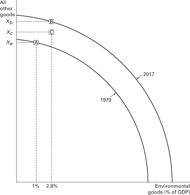
FIGURE 6.2 A Jobs– Environment Trade-Off?
However, again referring to your Econ 100 class, you know that until the 2008 recession, the U.S. economy was operating very close to full employment: at point B. And by 2016, the economy had largely recovered from the recession, with unemployment rates again below 5 percent. The point here is that economy-wide unemployment is determined by macroeconomic factors, not environmental regulation.
What kinds of jobs are generated by environmental spending? In fact, environmental protection provides employment heavily weighted to the traditional blue-collar manufacturing and construction sectors. Figure 6.3 illustrates this point, providing an estimated breakdown of the composition of nonagricultural jobs directly and indirectly dependent on environmental spending with comparative figures for the economy as a whole.
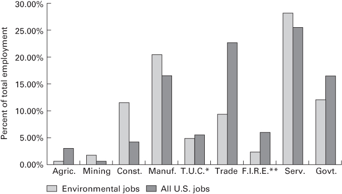
FIGURE 6.3 Jobs Dependent on Environmental Spending
* Transportation, utilities, and communication.
** Finance, insurance, and real estate.
Source: Author’s calculations from U.S. Environmental Protection Agency (1995) and Employment and Earnings, Washington, DC: U.S. Department of Labor. Data are from 1991.
While only 20 percent of all nonfarm jobs were in the manufacturing and construction sectors, 31 percent of employment generated by environmental spending fell in one of these categories. By contrast, only 12 percent of environment-dependent jobs were in wholesale and retail trade, finance, insurance, or real estate, compared to 29 percent for the economy as a whole. And despite the criticism that environmental regulation creates jobs only for pencil-pushing regulators, less than 12 percent of environmental employment was governmental, as compared to an economy-wide government employment rate of 17 percent.
How can we account for these results? Environmental protection is an industrial business. The private sector spends tens of billions of dollars on pollution-control plants and equipment and on pollution-control operations ranging from sewage and solid waste disposal to the purchase and maintenance of air-pollution-control devices on smokestacks and in vehicles. Federal, state, and local governments spend billions more on the construction of municipal sewage facilities. In addition, a very small percentage of all environmental spending supports the government’s direct regulation and monitoring establishment. The bulk of environmental spending thus remains in the private sector, generating a demand for workers disproportionately weighted to manufacturing and construction and away from services. This is not to say that environmental spending creates only high-quality, high-paying jobs. But, it does support jobs in traditional blue-collar industries.
GREEN JOBS
Of course, the several million jobs in the environmental industry are not the net jobs created. If the money had not been spent on environmental protection, it would have been spent elsewhere—perhaps on health care, travel, imported goods, or investment in new plants and equipment. This spending, too, would have created jobs. In the long run, the level of economy-wide employment is determined by the interaction of business cycles and government fiscal and monetary policy. However, in the short run, and locally, where we spend our dollars does matter for regions facing structural unemployment. As a rule, money spent on sectors that are both more labor-intensive (directly and indirectly) and have a higher domestic content (directly and indirectly) will generate more American jobs in the short run. Environmental spending is often labor-intensive or has a high domestic content.
To illustrate, a recent study examined a “green stimulus” package recommendation for the Obama administration that called for $100 billion of spending over 2 years on (1) retrofitting buildings to improve energy efficiency, (2) expanding mass transit and freight rail, (3) constructing a “smart” solar-powered electrical grid, and (4) investing in wind power and second-generation biofuels. The authors estimated that total jobs created would be 1.9 million. By contrast, if the money had simply been rebated to households to finance general consumption, only 1.7 million jobs would have been created. And if the $100 billion was spent on offshore drilling, only 550,000 jobs would have resulted. Again, “green” wins here because relative to the two alternatives, the proposed policies lower the imports of energy, rely on domestically produced inputs, and/or are more labor-intensive.9
Bottom line: most of the time, if you hear a sentence that begins with “All economists agree,” you should head for the door. But, in this case, there is agreement that, at the economy-wide level, there is simply no such thing as a jobs–environment trade-off.
LOCAL IMPACTS
Of course, this knowledge will not be comforting to the manufacturing or mining worker who has lost his or her job due to regulation. Short-run, structural unemployment impacts from environmental regulation (or any other cause) should not be minimized. Plant shutdowns cause considerable suffering for workers and communities, particularly for older workers who find it difficult to retool. Moreover, the disappearance of high-wage manufacturing jobs is indeed a cause for concern. Yet, fears of such effects from pollution-control efforts are liable to be greatly overblown as industry officials can politically gain by blaming plant shutdowns due to normal business causes on environmental regulations. Keeping this in mind, based on employer responses, the U.S. Department of Labor has collected information on the causes of mass layoffs (greater than 50 workers). Table 6.2 presents this data, covering 75 percent of all layoffs at large employers and 57 percent of all manufacturing plants.
TABLE 6.2 Sources of Mass Layoffs
Source: U.S. Bureau of Labor Statistics, Local Area Unemployment Statistics Division.
| Layoff Events | People Laid Off | |||||
| Reason for Layoff | 1995 | 1996 | 1997 | 1995 | 1996 | 1997 |
| Total, all reasons | 4,422 | 5,692 | 5,605 | 926,775 | 1,158,199 | 1,103,146 |
| Environment related* | 9 | 7 | 5 | 2,816 | 1,098 | 541 |
| Automation | 6 | 14 | 9 | 4,284 | 5,522 | 2,117 |
| Bankruptcy | 78 | 103 | 80 | 20,144 | 21,247 | 21,637 |
| Business ownership change | 120 | 167 | 121 | 28,482 | 46,425 | 25,141 |
| Contract cancellation | 103 | 87 | 61 | 18,700 | 19,269 | 11,813 |
| Contract completion | 459 | 557 | 759 | 100,289 | 124,506 | 175,572 |
| Domestic relocation | 63 | 76 | 76 | 11,059 | 11,323 | 15,241 |
| Financial difficulty | 249 | 263 | 153 | 58,473 | 56,749 | 39,634 |
| Import competition | 51 | 72 | 66 | 8,527 | 13,684 | 12,493 |
| Labor-management dispute | 20 | 32 | 32 | 3,370 | 14,119 | 16,149 |
| Material shortages | 19 | 21 | 14 | 2,666 | 2,821 | 1,705 |
| Model changeover | 17 | 18 | 18 | 7,589 | 6,799 | 5,716 |
| Natural disaster | 7 | 16 | 5 | 2,117 | 3,599 | 892 |
| Overseas relocation | 14 | 26 | 38 | 3,713 | 4,326 | 10,435 |
| Plant or machine repairs | 31 | 23 | 19 | 3,867 | 5,169 | 2,362 |
| Product line discontinued | 20 | 35 | 45 | 4,392 | 6,037 | 9,505 |
| Reorganization within company | 384 | 578 | 482 | 86,331 | 115,669 | 78,324 |
| Seasonal work | 1,688 | 2,173 | 2,434 | 385,886 | 488,398 | 499,331 |
| Slack work | 515 | 831 | 656 | 78,514 | 112,313 | 90,382 |
| Vacation period | 66 | 69 | 92 | 14,221 | 11,844 | 13,499 |
| Weather-related curtailment | 87 | 97 | 63 | 10,619 | 9,802 | 8,652 |
| Other | 253 | 266 | 211 | 42,153 | 55,265 | 39,821 |
| Not reported | 163 | 161 | 166 | 28,563 | 22,215 | 22,184 |
* Includes environmental and safety-related shutdowns.
On average, according to employers’ own estimates, environmental regulation accounted for less than one-tenth of 1 percent of all mass layoffs nationwide. In the survey, seven plants per year closed primarily as a result of environmental problems. If we double the figures to account for the remainder of manufacturing jobs, on average, 2,000 lost positions per year could be partially attributed to environmental regulation. Supporting this survey data, one very detailed study looked at a set of chemical and manufacturing plants (of all types) in heavily regulated southern California and then compared them with similar plants in the rest of the country. The study found no decrease in employment at the existing California plants and no effect on California jobs from increased bankruptcies or decreased investment. Indeed, the authors conclude: “In contrast to the widespread belief that environmental regulations cost jobs, the most severe episode of air quality regulation in the United States probably created a few jobs.”
That said, in individual cases, such as the restrictions imposed on the timber industry to protect the old-growth forest in the Pacific Northwest, or clean-air requirements faced by the Appalachian high-sulfur coal industry, local unemployment has been exacerbated by environmental regulation. Several thousand jobs were lost regionally over a few-year period of time. And beyond numbers, many of the jobs lost were relatively “good” union, high-paying ones, and reemployment opportunities for some workers were also quite limited. These negative effects should not be ignored, and they can be partially alleviated through government job-retraining programs or bridge financing to retirement.
POLLUTION HAVENS
The number of actual layoffs due to environmental regulation is clearly much smaller than is generally believed. As noted earlier, one-third of the entire U.S. workforce perceived a threat to their jobs from environmental protection measures! In reality, 40 times more layoffs resulted from ownership changes than from environmental measures.10 However, rather than shutdowns, one might expect new investment to occur in poorer countries with less-strict pollution regulations. How serious is this problem of flight to the so-called pollution havens?
“Studies conducted through the late 1990s found little impact of environmental regulation on trade flows. More recent evidence, however, has renewed the debate on the degree to which dirty industry has slowly migrated offshore. By carefully looking at the few U.S. industries that face high regulatory costs, and controlling the high shipping costs often associated with commodities produced by dirty industry, a pattern that shows a slow change in the composition of trade in pollution-intensive products that favors middle-income countries is emerging.11
This pollution-haven effect is not readily apparent, nor universal. For example, with its close proximity to the United States, the maquiladora region of northern Mexico would be a logical candidate to become a pollution haven. Yet, a comprehensive look at investment in the area confirms that environmental factors are, in general, relatively unimportant. Industries with higher pollution-abatement costs are not overrepresented in the maquiladora area, although those with higher labor costs are.
Why have the effects not been greater? First, pollution-control costs are a small portion of total business costs; and second, costs are only one factor influencing business-location decisions. In addition to costs, factors as diverse as access to markets and the quality of life are important components of business-location decisions. Market size, wages, tax rates, political stability, access to the European market, and distance to the United States are some of the primary determinants of U.S. investment abroad. Finally, much pollution-control technology is embedded in modern plant designs. This means that a chemical factory built by a multinational corporation in South China will, in fact, look a lot like one built in West Virginia. Given these factors, most U.S. direct foreign investment continues to be in developed countries with environmental regulations comparable to our own.12
This section has established that, first, economy-wide, net job loss has not resulted from environmental protection, as many, if not more, new jobs have been created than have been lost. At the national level, debates that assume a job versus the environment trade-off are thus based on pure myth. Second, gross job loss due to environmental protection has been surprisingly small. Approximately 2,000 workers per year have been laid off in recent years, partially as a result of regulation. Finally, the flight of U.S. manufacturing capital overseas appears to be driven much more by wage differentials than by stringent environmental rules. Despite these facts, the fear of job loss remains widespread, as indicated by the poll results cited earlier. Much of the political resistance to environmental protection remains motivated by such fears.
Generally, the issue of jobs is overstated in the discussions of environmental protection. Large numbers of jobs are, typically, neither gained nor lost, when new regulations come into force. As a result, while there will be a slow shift in the types of jobs as a nation devotes more resources to environmental protection, this shift does not add to the dollar costs, or increase the dollar benefits, from environmental protection.
6.4 General Equilibrium Effects and the Double Dividend
The last important area in which there may be “hidden” costs (or benefits) of regulation lies in what economists call general equilibrium (GE) effects. These effects of regulation are felt throughout the economy, as opposed to the effects felt in the specific regulated sector (partial equilibrium effects).
To make this issue concrete, suppose that you were working at the EPA and trying to figure out the cost of a new air-quality regulation on coal-burning power plants. To simplify matters, first assume that there are 100 coal plants nationwide and each would install scrubbers, costing $100 million apiece. In that case, the estimated cost of the regulation would be $10 billion (100 plants × $100 million). Yet, even ignoring other compliance options (such as switching to low-sulfur coal), this would be only a partial equilibrium estimate.
In fact, the higher cost of electricity would reduce electricity demand, as people conserved more. Hence, utilities would probably retire rather than retrofit some of the coal plants, leading to lower overall costs. Taking into account the general equilibrium effects in the electricity market, the real costs of the regulation would be lower than your partial equilibrium estimate. Of course, you would also want to calculate impacts of higher electricity prices throughout the economy. Probably, the most significant general equilibrium effect runs through the so-called double-dividend hypothesis. The idea here is that a pollution tax can have two beneficial effects on the economy. The first impact is to internalize the externality, so that firms and consumers stop over-consuming “dirty” goods. The second impact flows through beneficial use of the tax revenue. For example, suppose that carbon tax revenues were used to cut payroll taxes on labor. This would encourage firms to hire more workers. By shifting taxes from “good things” to “bad things,” pollution fees could lower the overall cost to the economy of cleaning up the environment.
While the double-dividend idea is intuitively appealing, some economists have questioned the size and even the existence of the effect. This is because a pollution tax on coal emissions, for example, raises the costs of unrelated goods and services (e.g., medical services from a hospital that depends on coal-fired electricity). Higher prices for goods and services can then feed back to reductions in consumption and, potentially, reduced labor supply.
Piling up these kinds of interrelated, theoretical interactions can quickly cause one’s head to spin. General equilibrium effects are difficult to comprehend, or to assess definitively, because they are quite complicated. And from a policy perspective, precisely because these general equilibrium costs (and benefits) are so deeply hidden, no one besides (a few) economists currently cares much about them. Nevertheless, these indirect costs—if they could be reliably measured—are as real as the more obvious direct ones. The take-home message of this section is, again, that a careful reckoning of environmental protection costs can be as difficult as developing good benefit measures.
6.5 A Final Look at Benefit– Cost Analysis
We will end this chapter with a real-world look at a recent EPA benefit–cost effort, a 2011 Regulatory Impact Analysis completed in support of rules that require coal-fired electric utilities to reduce mercury emissions. (Read why this regulation was delayed for 40 years before coming into force, in Chapters 12 and 17!) Here, we reproduce the Executive Summary, Table 6.3, and the RIA punchline from the first paragraph. (PM2.5 refers to particulate matter of 2.5 microns or larger in size).13
TABLE 6.3 Summary of the EPA’s Estimates of Annualized Benefits, Costs, and Net Benefits of the Final MATS in 2016 (billions of 2007$)
| Description | Estimate |
| Costs | $9.6 |
| Benefits | $37–$90+ “B”* |
| Net benefits | $27–$80+ “B”* |
*“B” represents unquantified benefits. See the related discussion.
This rule will reduce emissions of Hazardous Air Pollutants (HAP), including mercury, from the electric power industry. As a co-benefit, the emissions of certain PM2.5 precursors such as will also decline. EPA estimates that this final rule will yield annual monetized benefits (in 2007$), of between $37 and $90 billion. The great majority of the estimates are attributable to co-benefits from 4,200 to 11,000 fewer PM2.5-related premature mortalities. The monetized benefits from reductions in mercury emissions, calculated only for children exposed to recreationally caught freshwater fish, were expected to be $0.004 to $0.006 billion in 2016 using a 3 percent discount rate and $0.0005 to $0.001 billion using a 7 percent discount rate. The annual social costs, approximated by the compliance costs, are $9.6 billion (2007$), and the annual monetized net benefits are $27 to $80 billion. The benefits outweigh costs by between 3 and 1 or 9 and 1, depending on the benefit estimate and discount rate used. There are some costs and important benefits that EPA could not monetize, such as other mercury reduction benefits and those for the HAP other than mercury being reduced by this final rule. Upon considering these limitations and uncertainties, it remains clear that the benefits of the MATS are substantial and far outweigh the costs. Employment impacts associated with the final rule are estimated to be small.
There is a lot of complexity in this paragraph, but from what we have learned in the previous two chapters, we are ready to tackle it piece by piece. Note first that the benefits and costs are “annualized”—Table 6.3 reports the expected benefits and costs of cleaning up on a yearly basis, instead of the sum of all benefits and costs over time. More on this to follow.
Costs. The EPA took a “simple” approach to measuring costs: “Total social costs are approximated by the compliance costs.” To get at this, EPA used detailed models of the oil- and coal-fired electricity-generating sectors to estimate the direct costs of installing pollution-control equipment; the number of older plants liable to shutdown; and the costs imposed on electricity users due to slightly higher electricity prices. The agency also included monitoring, reporting, and recordkeeping costs. Note there is NO uncertainty bound reported for costs: the EPA felt comfortable with the $9.6 billion per year cost estimate.
That said, and hitting the themes of this chapter, at the end of the Executive Summary, the EPA notes:
- Compliance costs are used to approximate the social costs of this rule. Social costs may be higher or lower than compliance costs and differ because of preexisting distortions in the economy and because certain compliance costs may represent shifts in rents. [What we called General Equilibrium impacts.]
- Analysis does not capture employment shifts as workers are retrained at the same company or re-employed elsewhere in the economy.
- Technological innovation is not incorporated into these cost estimates. Thus, these cost estimates may be potentially higher than what may occur in the future, with all other things being the same.
These cost uncertainties highlight the difference between engineering cost estimates of compliance and the true social opportunity cost. And as always, there is a lot of wiggle room for partisan attacks on the EPA’s methodology: industry critics of the mercury rule argued that compliance costs, and costs to industries affected by higher electricity prices, could be three times as high as that the EPA asserted.14
Costs were annualized using a 6.15 percent discount rate: this means that $9.6 billion is the annual cost to firms and electricity users for around 20 years. For example, if electric utility firms borrowed the money upfront to pay the total cost of all the new equipment they needed to cut emissions in year 1, they would have to pay $9.6 billion in principal and interest for about 20 years to pay off the initial cost.
Benefits. The RIA acknowledges HUGE uncertainty here. First, the range of $37–$90 billion reflects only two benefits: reductions in cognitive impacts on children exposed to mercury from eating fish and reductions in premature death and sickness from a “co-benefit” of the mercury rules: reductions in tiny particles (PM2.5) that cause respiratory illnesses and heart disease. In fact, 99 percent of the measured benefits were from this second category and had nothing to do with direct reductions in mercury!
In particular, the EPA concluded that the regulations, per year, would result in “510 fewer mercury-related IQ points lost as well as avoided PM2.5-related impacts, including 4,200 to 11,000 premature deaths, 4,700 nonfatal heart attacks, 2,600 hospitalizations for respiratory and cardiovascular diseases, 540,000 lost workdays, and 3.2 million days when adults restrict normal activities because of respiratory symptoms exacerbated by PM2.5. We also estimate substantial additional health improvements for children from reductions in upper and lower respiratory illnesses, acute bronchitis, and asthma attacks.”
The 510 IQ points gained annually by children were calculated by (1) estimating the contaminated fish consumption and mercury exposure and (2) assuming a dose–response function by which decreased mercury exposure leads to higher IQ. The IQ increase from less contamination was in turn valued at $4–$6 million, based on an estimated increase in net lifetime earning less the cost of remedial schooling. (Imagine the uncertainty in each of these steps!) The reductions in mortality of 4,200 to 11,000, again based on scientific models, and using a statistical value of life of $8 million for each death averted, weighed in at $34 to $87 billion. The additional health benefits identified earlier—reduced sickness, lost workdays, and restricted activity days—rounded out the additional $3 billion in annual benefits. A general point to be drawn here: reductions in premature mortality tend to generate the largest regulatory benefits.
Is mercury reduction itself only valued at $4 to $6 million annually? No. That’s where the “+B”—representing unquantified benefits—in Table 6.3 comes in. The RIA lists three full pages of benefits that the EPA did not even try to quantify, with the following categories:
- Reduced incidence of mortality from exposure to ozone
- Reduced incidence of morbidity from exposure to ozone, , and
- Reduced visibility impairment
- Reduced climate effects
- Reduced effects on materials
- Reduced effects from PM deposition (metals and organics)
- Reduced vegetation and ecosystem effects from exposure to ozone
- Reduced effects from acid deposition
- Reduced effects from nutrient enrichment
- Reduced vegetation effects from ambient exposure to and
For mercury, unquantified benefits for human health included other neurologic effects beyond IQ loss (e.g., developmental delays, memory, behavior); cardiovascular effects; and genotoxic, immunologic, and other toxic effects. Neither did the study attempt to quantify the value of improved fish and wildlife health from reduced mercury exposure, nor the benefits to commercial and recreational fishing and hunting.
Why did the EPA list but not quantify all these additional benefits? In part, because it is difficult and expensive to do so. And in part, because the health co-benefits of PM2.5 were so large that, without quantifying all the other impacts, and despite the large uncertainties, the rule clearly passes a benefit–cost test. That said, without the PM2.5 co-benefits, it is unlikely that mercury reductions alone would have justified the regulation from a benefit–cost perspective.
Jobs. The RIA concludes that employment impacts of the rule in the regulated sector itself will be small. In fact, the EPA estimates small net job increases to be more likely, giving a range of to +30,000. At the same time, the study estimated that short-term manufacture and installation of the required pollution-control equipment would create 46,000 jobs. Of course, these job gains would need to be balanced against jobs slowly lost as a result of higher electricity prices outside of the regulated sector or slowly gained as low-mercury electric generation capacity came on line. Consistent with the discussion earlier in this chapter, jobs created or lost to environmental regulation are generally not large enough in number to determine policy.
In this section, we have brought some of our recently gained knowledge to bear in helping us understand how the EPA uses benefit–cost analysis. Again, in real-world application, especially on the benefits side, uncertainty will always loom large. Despite that, when regulations will save a lot of lives, we can often assert with some confidence that benefits do exceed costs.
6.6 Summary
This chapter has explored the different ways to evaluate the costs of environmental protection. Engineering cost data are much easier to obtain compared to nonmarket benefit information; as a result, the EPA has been able to put a price tag of close to 3 percent of GDP on our federal, state, and local pollution-control efforts.
However, even on their own terms, engineering cost estimates are only as good as their predictions regarding, for example, compliance and control technologies. More significantly, engineering estimates do not generally incorporate indirect effects, such as negative or positive productivity impacts or general equilibrium effects. On the productivity front, the overall costs of protecting the environment will be lower if firms respond to regulations by better managing risk, becoming more resource-efficient, and investing in new areas of profitable innovation, replacing polluting products and processes. In addition environmental protection can lower economy-wide health costs. On the flip side, increasing end-of-the-pipe control costs can eat up the funds for investment, and cause prices to rise for industries that depend on dirty goods, with a similar effect. Red tape and regulatory delay can also slow down investment and innovation. On balance, the net, economy-wide impact on productivity has probably been small. Nevertheless, small declines in productivity growth have big long-run effects and should be a primary concern in regulatory design.
On the employment front, environmental regulation has not led to any net job loss in the economy; there is simply no evidence of a long-run “jobs versus the environment” trade-off. Instead, regulation has led to a shift in the types of jobs. Rather surprisingly, regulation-induced employment is heavily weighted to manufacturing and away from services. And when green spending has more domestic content or is labor-intensive, it can lead to net employment growth in the creation of “green jobs.” Gross job losses partially due to environmental protection in the 1990s were on the order of 1,500 to 2,000 per year. Finally, there is little evidence to support widespread capital flight to “pollution havens.”
Environmental policy can change prices throughout the economy, altering firm and consumer behavior. In particular, if pollution taxes or permit auction revenues are used to cut other taxes, then the emerging double dividend can lower the overall cost to the economy of achieving environmental or resource protection.
Due to these three different indirect effects, the “true” social cost of regulation (its opportunity cost) may vary widely from engineering cost estimates. This point again highlights the relative imprecision of benefit–cost analysis for determining the “efficient” pollution level. We ended this chapter with a look at a real-world benefit–cost analysis at the EPA. Mercury regulations were expected to cost, on an annual basis, $9.6 billion and generate benefits ranging from $37 to $90 billion, plus “B,” unquantified benefits. This case illustrates that large benefits emerge for the regulation expected to significantly reduce premature deaths. In addition while the study is careful in highlighting the uncertainty on the benefits side, it illustrates a hard numbers illusion on the cost side. In part, this is the EPA seeking to defend the rule from industry attacks. Despite of the lack of an official uncertainty bound, industry groups still put the possible cost of the regulations at three times the EPA’s estimate and characterize the rule as the most expensive in the history of regulation.
The previous three chapters have explored in much detail the first answer to the question: How much pollution is too much? Efficiency advocates argue that environmental policy measures must pass a benefit–cost test and indeed, weighing the costs against the benefits of cleanup, deliver the maximum net dollar benefits to society. To do this, of course, one needs to be able to measure both the dollar benefits and dollar costs of environmental protection with some accuracy. We have seen that this task can be quite difficult. So, even after assuming that efficiency is indeed the correct ethical goal for environmental cleanup, there is an open question as to how well we can effectively implement it. Next, we turn our attention to an alternate answer to the How Much is Too Much question, an answer that underlies most current U.S. policy: The Safety Standard.
KEY IDEAS IN EACH SECTION
- 6.0 The standard method of estimating the costs of environmental protection, simply adding up direct compliance and regulatory expenses, is called an engineering approach. Economists, however, would like to measure the opportunity cost the value of goods and services forgone by investing in environmental protection. Opportunity costs include three indirect effects: productivity impacts, employment impacts, and general equilibrium effects.
- 6.1 In 2000, the United States spent about $260 billion on pollution-control measures, measured in engineering terms. Between 1970 and 2000, environmental protection expenditures jumped from less than 1 percent to more than 2.8 percent of GNP, more than doubling their claim on the share of the nation’s resources.
- 6.2 The productivity slowdown of the 1970s has been partially blamed on environmental regulation. The main argument is that regulatory expenses divert investment from new plants and equipment. Several economic studies indicate that a small portion of the slowdown (less than 10 percent) may be due to environmental protection measures. However, this does not take into account the possible positive impacts on productivity growth from more efficient resource use, Porter hypothesis effects, or a healthier population and resource base. Nevertheless, even small negative effects on productivity growth can impose large costs in the long run.
- 6.3 This section reviews the employment impact of environmental regulation and states four main points. First, at the economy-wide level, environmental protection has not generated a jobs–environment trade-off. Moreover, investment in green jobs can lead to net job growth in some cases. Third, extrapolating data from a large sample of employer responses, gross job loss from plant shutdowns due to environmental regulation was about 1,500 to 2,000 workers per year during the 1990s. Therefore, little structural unemployment can be attributed to regulation. Finally, it appears that in only a few cases have U.S. firms relocated investment to in pollution havens primarily to avoid environmental regulations.
- 6.4 A final source of hidden costs and benefits for measures to protect the environment and the resource base arises from general equilibrium effects. Such impacts arise as regulation alters the prices, not just for the regulated commodity but throughout the economy, causing firms and consumers to change their behaviors. The major general equilibrium impact of pollution taxes or for government-auctioned permits under cap and trade, works through the double-dividend hypothesis, in which pollution tax or permit revenues are used to cut taxes on labor, leading to greater levels of employment.
- 6.5 The benefit–cost analysis (regulatory impact statement) done by the EPA for mercury control from power plants highlights the uncertainty associated with estimating benefits and illustrates the hard numbers illusion with respect to costs. The RIA also affirmed the general point that effects of jobs—both positive and negative—associated with environmental policy measures are small and tend to balance each other out.
REFERENCES
- Ambec, Stefan, Mark A. Cohen, Stewart Elgie, and Paul Lanoie. 2011. The Porter hypothesis at 20 can environmental regulation enhance innovation and competitiveness? Discussion paper 11-01. Washington, DC: Resources for the Future.
- Baumol, William, and Alan Blinder. 1991. Macroeconomics: Principles and policy. New York: Harcourt Brace Jovanovich.
- Beach, William, David Kreutzer, Karen Campbell, and Ben Lieberman. 2009. Son of Waxman-Markey: More politics makes for a more costly bill. Heritage Foundation, WebMemo 2450, 18 May.
- Boyd, Gale, and John McClelland. 1999. The impact of environmental constraints on productivity improvement in integrated paper plants. Journal of Environmental Economics and Management 38(2): 121–42.
- Brunnermeier, Smita B., and Arik Levinson. 2004. Examining the evidence on environmental regulations and industry location. Journal of Environment & Development 13(1): 6–41.
- Carlin, Alan. 1990. Environmental investments: The cost of a clean environment, Summary. Washington, DC: U.S. EPA.
- EPA plans to tighten pollution rules. 1997. Wall Street Journal, 6 June, A16.
- Goodstein, Eban. 1999. The trade-off myth: Fact and fiction about jobs and the environment. Washington, DC: Island Press.
- Graff Zivin, Joshua, and Matthew J. Neidell. 2011. The impact of pollution on worker productivity NBER working paper no. 17004, Issued in April.
- Grossman, Gene M., and Alan B. Krueger. 1995. Economic growth and the environment. Quarterly Journal of Economics 110(2): 353–77.
- Harrington, Winston, Richard Morgenstern, and Peter Nelson. 1999. Predicting the costs of environmental regulation. Environment 41(7): 10–14.
- King County (2015) King County Strategic Climate Action Plan, November (King County, Seattle, WA) http://your.kingcounty.gov/dnrp/climate/documents/2015_King_County_SCAP-Full_Plan.pdf
- Morgenstern, Richard, William Pizer, and Jhih-Shyang Shih. 1997. Are we overstating the real costs of environmental protection? Discussion paper 97-36-REV. Washington, DC: Resources for the Future.
- Pollin, Robert, Heidi Garrett-Peltier, James Heintz, and Helen Scharber. 2008. Green recovery: A program to create good jobs and start building a low-carbon economy. Amherst: University of Massachusetts Political Economy Research Institute.
- Porter, Michael, and Claas van der Linde. 1995. Toward a new conception of the environment-competitiveness relationship. Journal of Economic Perspectives 9(4): 97–118.
- Sturmak, Bud, and Cary Krosinsky. 2011. “On performance” in evolutions in sustainable investing, ed. Cary Krosinsky. New York: Wiley.
- U.S. Environmental Protection Agency. 1995. The U.S. environmental protection industry: A proposed framework for assessment. Washington, DC: U.S. EPA, Office of Policy Planning and Evaluation.
- Xepapadeas, Anastasios, and Aart de Zeeuw. 1999. Environmental policy and competitiveness: The Porter hypothesis and the composition of capital. Journal of Environmental Economics and Management 37(2): 165–82.