In this final chapter of Part One we shall discuss some more specialized topics, which will be applied later in this book. These include some further results on adjoint matrices (Sections 3.2 and 3.3), Hadamard products (Section 3.6), the commutation and the duplication matrix (Sections 3.7–3.10), and some results on the bordered Gramian matrix with applications to the solution of certain matrix equations (Sections 3.13 and 3.14).
2 THE ADJOINT MATRIX
We recall from Section 1.9 that the cofactor cij of the element aij of any square matrix A is (−1)i+j times the determinant of the submatrix obtained from A by deleting row i and column j. The matrix C = (cij) is called the cofactor matrix of A. The transpose of C is called the adjoint matrix of A and we use the notation
(1)
We also recall the following two properties:
(2)
(3)
Let us now prove some further properties of the adjoint matrix.
Before giving the proof of Theorem 3.1, we formulate the following two consequences of this theorem.
A direct proof of Theorem 3.3 is given in the Miscellaneous Exercises 5 and 6 at the end of Chapter 8.
Exercises
1.
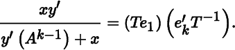
Why is y′x ≠ 0 in (7)?
2.
Show that y′x = 0 in (5) if k ≥ 2.
3. (i) (ii) (iii) Let A be an n × n
(i) ∣A# ∣ = |A|n − 1(n ≥ 2),
(ii) (αA)# = αn − 1A# (n ≥ 2),
(iii) (A#)# = |A|n − 2A (n ≥ 3).
3 PROOF OF THEOREM 3.1
If r(A) = n, the result follows immediately from (2). To prove that A# = 0 if r(A) ≤ n − 2, we express the cofactor cij as
where Ej is the n × (n − 1) matrix obtained from In by deleting column j. Now, is an (n − 1) × (n − 1) matrix whose rank satisfies
It follows that is singular and hence that cij = 0. Since this holds for arbitrary i and j, we have C = 0 and thus A# = 0.
The difficult case is where r(A) = n − 1. Let λ1, λ2, …, λn be the eigenvalues of A, and assume
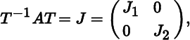
while the remaining n − k eigenvalues are nonzero. By Jordan's decomposition theorem (Theorem 1.14), there exists a nonsingular matrix T such that
(8)
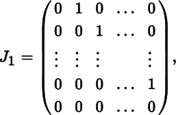
where J1 is the k × k matrix
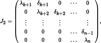
J2 is the (n − k) × (n − k) matrix
and δj (k + 1 ≤ j ≤ n − 1) can take the values 0 or 1 only.
It is easy to see that every cofactor of J vanishes, with the exception of the cofactor of the element in the (k, 1) position. Hence,
(9)
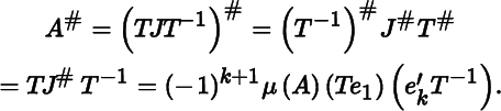
where e1 and ek are the first and kth elementary vectors of order n × 1, and μ(A) denotes the product of the n − k nonzero eigenvalues λk+1, …, λn of A. (An elementary vector ei is a vector with one in the ith position and zeros elsewhere.) Using (3), (8), and (9), we obtain
(10)
Since the first column and the kth row of J1 are zero, we have Je1 = 0 and . Hence,
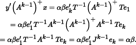
Further, since r(A) = n − 1, the vectors x and y satisfying Ax = A′y = 0 are unique up to a factor of proportionality, that is,
1.
Prove that |A + αıı′| = |A| + αı′A#ı (Rao and Bhimasankaram 1992).
5 THE MATRIX EQUATION AX = 0
In this section, we will be concerned in finding the general solutions of the matrix equation AX = 0, where A is an n × n matrix with rank n − 1.
6 THE HADAMARD PRODUCT
If A = (aij) and B = (bij) are matrices of the same order, say m × n, then we define the Hadamard product of A and B as
Thus, the Hadamard product A ⊙ B is also an m × n matrix and its ijth element is aijbij.
The following properties are immediate consequences of the definition:
(14)
(15)
(16)
so that the brackets in (16) can be deleted without ambiguity. Further,
(17)
(18)
(19)
where J is a matrix consisting of ones only.
The following two theorems are of importance.
7 THE COMMUTATION MATRIX Kmn
Let A be an m × n matrix. The vectors vec A and vec A′ contain the same mn components, but in a different order. Hence, there exists a unique mn × mn permutation matrix which transforms vec A into vec A′. This matrix is called the commutation matrix and is denoted by Kmn or Km,n. (If m = n, we often write Kn instead of Knn.) Thus,
(20)
Since Kmn is a permutation matrix, it is orthogonal, i.e. , see Equation ( 13
) in Chapter 1. Also, premultiplying (20) by Knm gives
The key property of the commutation matrix (and the one from which it derives its name) enables us to interchange (commute) the two matrices of a Kronecker product.
An important application of the commutation matrix is that it allows us to transform the vec of a Kronecker product into the Kronecker product of the vecs, a crucial property in the differentiation of Kronecker products.
Closely related to the matrix Kn is the matrix , denoted by Nn. Some properties of Nn are given in Theorem 3.11.
Exercise
1. Let A (m × n) and B (p × q) be two matrices. Show that
where
8 THE DUPLICATION MATRIX Dn
Let A be a square n × n matrix. Then vech(A) will denote the vector that is obtained from vec A by eliminating all supradiagonal elements of A (i.e. all elements above the diagonal). For example, when n = 3:
and
In this way, for symmetric A, vech(A) contains only the generically distinct elements of A. Since the elements of vec A are those of vech(A) with some repetitions, there exists a unique matrix which transforms, for symmetric A, vech(A) into vec A. This matrix is called the duplication matrix and is denoted by Dn. Thus,
(22)
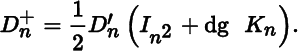
Let A = A′ and Dn vech(A) = 0. Then vec A = 0, and so vech(A) = 0. Since the symmetry of A does not restrict vech(A), it follows that the columns of Dn are linearly independent. Hence, Dn has full column rank , is nonsingular, and , the Moore‐Penrose inverse of Dn, equals
(23)
Since Dn has full column rank, vech(A) can be uniquely solved from (22) and we have
(24)
Some further properties of Dn are easily derived from its definition ( 22
).
Much of the interest in the duplication matrix is due to the importance of the matrices and , some of whose properties follow below.
Finally, we state, without proof, two further properties of the duplication matrix which we shall need later.
9 RELATIONSHIP BETWEEN Dn+1 AND Dn, I
Let A1 be a symmetric (n + 1) × (n + 1) matrix. Our purpose is to express and as partitioned matrices. In particular, we wish to know whether is a submatrix of and whether is a submatrix of when A is the appropriate submatrix of A1. The next theorem answers a slightly more general question in the affirmative.
10 RELATIONSHIP BETWEEN Dn+1 AND Dn, II
Closely related to Theorem 3.15 is the following result.
11 CONDITIONS FOR A QUADRATIC FORM TO BE POSITIVE (NEGATIVE) SUBJECT TO LINEAR CONSTRAINTS
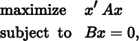
Many optimization problems take the form
and, as we shall see later (Theorem 7.12) when we try to establish second‐order conditions for Lagrange minimization (maximization), the following theorem is then of importance.
12 NECESSARY AND SUFFICIENT CONDITIONS FOR r(A : B) = r(A) + r(B)
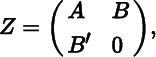
Let A be a positive semidefinite n × n matrix and B an n × k matrix. The symmetric (n + k) × (n + k) matrix
called a bordered Gramian matrix, is of great interest in optimization theory. We first prove Theorem 3.20.
Next we obtain the Moore‐Penrose inverse of Z.
In the special case where ℳ(B) ⊂ ℳ(A), the results can be simplified. This case is worth stating as a separate theorem.
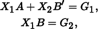
14 THE EQUATIONS X1A + X2B′ = G1, X1B = G2
The two matrix equations in X1 and X2,
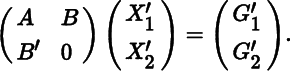
where A is positive semidefinite, can be written equivalently as
The properties of the matrix Z studied in the previous section enable us to solve these equations.
An important special case of Theorem 3.23 arises when we take G1 = 0.
Exercise
1.
Give the general solution for X2 in Theorem 3.24.
MISCELLANEOUS EXERCISES
1.
2.
3.
4. Let ei denote an elementary vector of order m, that is, ei has unity in its ith position and zeros elsewhere. Let uj be an elementary vector of order n. Define the m2 × m and n2 × n matrices
Let A and B be m × n matrices. Prove that
BIBLIOGRAPHICAL NOTES
2. A good discussion on adjoint matrices can be found in Aitken (1939, Chapter 5). Theorem 3.1(b) appears to be new.
6. For a review of the properties of the Hadamard product, see Styan (1973). Browne (1974) was the first to present the relationship between the Hadamard and Kronecker product (square case). Faliva (1983) and Liu (1995) treated the rectangular case. See also Neudecker, Liu, and Polasek (1995); Neudecker, Polasek, and Liu (1995); and Neudecker and Liu (2001a,b) for a survey and applications of the Hadamard product in a random environment.
7. The commutation matrix was systematically studied by Magnus and Neudecker (1979). See also Magnus and Neudecker (1986). Theorem 3.10 is due to Neudecker and Wansbeek (1983). The matrix Nn was introduced by Browne (1974). For a rigorous and extensive treatment, see Magnus (1988).
8. See Browne (1974) and Magnus and Neudecker (1980, 1986) for further properties of the duplication matrix. Theorem 3.14 follows from Equations (60), (62), and (64) in Magnus and Neudecker (1986). A systematic treatment of linear structures (of which symmetry is one example) is given in Magnus (1988).