7
Economics of Manufacturing Pollution Prevention: Toward an Environmentally Sustainable Industrial Economy
7.1 Introduction
The failure of many pollution‐prevention programs can be traced to the inability of the engineers and scientists to convince business leadership to change manufacturing processes unfavorable to the environment. Often, this reluctance to change is not because the recommended process improvements were technically unsound, but because the engineering team failed to speak the language of business, that is dollars and cents. The role of economics in pollution prevention is very important, even as important as the ability to identify technologies changes to the process, new and emerging technologies, process and/or product modification, Zero Discharge technologies, technologies for biobased engineered chemicals, products, renewable energy sources, and its associated costs.
Market acceptance of new technologies, products, processes, and services depend upon the complex interplay of cost, physical properties, environmental performance, public policy, cultural prejudices, and other factors. Accurate forecasting is a difficult and time‐consuming activities best left to the experts. However, cost estimating is a valuable skill that allows an engineer to obtain “ballpark” approximation of project costs. The goal is to obtain an estimate that is within ±30% of the actual cost if the enterprise were pursued. Such estimates are relatively easy to develop. Engineers use a relatively small set of financial tools to assess alternative capital investments and to justify their selections to upper management. Most often, the engineer's purpose is to show how a recommended investment will improve the company's profitability. Spending on capital improvements is largely voluntary. Adding an assembly line or changing from one type of gasket material to another can be postponed, or the proposal, or rejected outright. This is not the case with pollution control devices, which are necessary for compliance with state and federal pollution standards and generally must be installed by or before a mandated deadline. Consequently, a decision to install device X may not originate with the engineer. Instead, the need for pollution control equipment might be identified by a company's environmental manager who then passes the decision to acquire device X down to the engineer. This chapter gives some cost‐estimating methods that can be used to assess the costs of implementing pollution prevention technologies; these methods are useful, as well, in cost comparisons, and in considerations of cost‐effectiveness, best available technologies and emerging technologies. Also provided is some information about the cost of renewable resources and the cost of manufacturing biobased products from such feedstocks. We begin, however, with a few remarks about the economic matrix in which profitable pollution control technology and best control technology are implemented.
7.2 Economic Evaluation of Pollution Prevention
The economic evaluation of engineering projects typically involves estimation of equipment, installation, raw material, energy, and maintenance cost. Disposal and pollution control costs are often factored into these calculations in determining economic rates of return, but other regulatory and social costs are not. In this chapter, total cost assessment of waste management alternatives is described, and the hidden costs, future liabilities, and less tangible costs associated with waste generation are discussed.
7.2.1 Total Cost Assessment of Pollution Control and Prevention Strategies
Traditional economic measure of engineering projects evaluate equipment, raw‐material, energy, operating, and maintenance costs. These evaluations generally overlook some of the costs of waste generation. A more complete accounting of environmental costs is referred to as total cost assessment. Four types of costs are identified, which are labeled as tier 0, tier 1, tier 2, and tier 3. Tier 0 costs are the “usual” costs that are included in a conventional analysis of a project. Tier 1 costs are included in a conventional analysis of a project. Tier 1 costs include permitting, reporting, monitoring, manifesting, and insurance costs and are often referred to as “hidden” costs because they are usually treated as overhead costs and are not directly charged to a project. Waste disposal costs are sometimes treated as overhead costs as well. Tier 2 costs include future liabilities, which are extremely difficult to accurately evaluate. Even more difficult to evaluate are tier 3 costs, which include consumer responses, employee relations, and public image. All four tiers of costs provide information for financial analysis methods, where measures such as ROR and payback periods (PPs) are evaluated.
7.2.2 Economics of Pollution Control Technology
In the present economic system, the goal of a sustainable development process is to maintain intergenerational equity by ensuring quality of life for future generations, which essentially requires the stopping of further damage to the environment. From this point of view the necessity of an integrated system consisting of modern manufacturing production and controlling technologies is being gradually recognized. To this end, various regulatory measures are being implemented, mainly in the industrial sector, which is the major contributor of pollution, for adopting such technologies.
7.3 Cost Estimates
The costs and estimating methodology in this section are directed toward the “study” estimate with a nominal accuracy of ±30%. According to Perry's Chemical Engineer's Handbook, a study estimate is “used to estimate the economic feasibility of a project before expending significant funds for piloting, marketing, land surveys, and acquisition. However, it can be prepared at relatively low cost with minimum data” (Perry and Green 1997). Specifically, the development of a study estimate calls for knowledge of the following:
- Location of the source within the plant
- Rough sketch of the process flow sheet (i.e. the relative locations of the equipment in the system)
- Preliminary sizes of, and material specifications for, the system equipment items
- Approximate sizes and types of construction of any buildings required to house the control system
- Rough estimates of utility requirements (e.g. electricity)
- Preliminary flow sheet and specifications for ducts and piping
- Approximate sizes of motors required
In addition, since the accuracy of an estimate (study or otherwise) depends on the amount of engineering work expended on the project, the user will need an estimate of the labor hours required for engineering and drafting activities. There are four other types of estimate.
The order‐of‐magnitude estimate, a rule‐of‐thumb procedure, can be used only for plant installations of the repetitive type for which there exists good cost history. Its error bounds are greater than ±30%. (However, Perry states that “no limits of accuracy can safely be applied to [an order‐of‐magnitude estimate].”) The sole input required for making an order‐of‐magnitude estimate is the control system's capacity (often measured by the maximum volumetric flow rate of the gas passing through the system).
The other three types of estimate, listed next, are preferable.
- Scope, budget authorization, or preliminary. This estimate, nominally of ±20% accuracy, requires more detailed knowledge than the study estimate regarding the site, flow sheet, equipment, buildings, etc. In addition, rough specifications for the insulation and instrumentation are also needed.
- Project control or definitive. These estimates, accurate to within ±10%, require yet more information than the scope estimates, especially concerning the site, equipment, and electrical requirements.
- Firm or contractor's or detailed. This is the most accurate (±5%) of the estimate types, requiring complete drawings, specifications, and site surveys. Consequently, detailed cost estimates are typically not available until right before construction. Common sense suggests that there is seldom enough time to prepare such estimate before approval to proceed with the project has been obtained.
7.3.1 Elements of Total Capital Investment
Total capital investment (TCI) includes all costs required to purchase equipment needed for the control system (purchased equipment costs), the costs of labor and materials for installing that equipment (direct installation costs), costs for site preparation and buildings, and certain other costs (indirect installation costs). TCI also includes costs for land, working capital, and off‐site facilities.
Direct installation costs include costs for foundations and supports, erecting and handling the equipment, electrical work, piping, insulation, and painting. Typical indirect installation costs are engineering costs, construction and field expenses (i.e. costs for construction supervisory personnel, office personnel, rental of temporary offices, etc.), contractor fees (for construction and engineering firms involved in the project), start‐up and performance test costs (to get the control system running and to verify that it meets performance guarantees), and associated costs with contingencies. “Contingencies” is a catch‐all category that covers unforeseen costs that may arise if, for example, it becomes necessary to redesign, modify equipment, to pay higher costs of equipment or field labor costs, or to compensate for delays in start‐up. Contingency costs are not the same as uncertainty and retrofit factor costs.
The elements of TCI are displayed in Figure 7.1. Note item “battery limits” cost, which is the sum of the purchased equipment cost, direct and indirect installation costs, and costs of site preparation and buildings. By definition, this is the total estimate for a specific job; any support facilities that may be needed (e.g. control systems) are assumed to already exist at the plant and are not included in the battery limits. For systems installed in new plants, off‐site facilities (special facilities for supporting the control system) also might be excluded from the battery limits. Off‐site facilities are exemplified by units to produce steam, electricity, and treated water; laboratory buildings; and railroad spurs, roads, and other transportation infrastructure items. Pollution control devices rarely consume enough energy to warrant dedicated off‐site capital units. However, it may be necessary – especially in the case of control systems installed in new or “grassroots” plants – to build extra capacity into the site's generating plant to service the system. (A Venturi scrubber, which often requires large amounts of electricity, is a good example.) Nevertheless, that the capital cost of a device does not include utility costs, even if the device were to require an offsite facility. Utility costs are charged to the project as operating costs at a rate that covers both the investment and operating and maintenance costs for the utility.
As Figure 7.1 shows, the installation of pollution control equipment may also require land, but since most add‐on control systems take up very little space (a quarter‐acre or less), this cost tends to be relatively small. Certain control systems, such as those used for flue‐gas desulfurization or selective catalytic reduction (SCR), require larger quantities of land for the equipment, chemicals storage, and waste disposal. In these cases, especially when a retrofit installation must be performed, space constraints can significantly influence the cost of installation, and the purchase of additional land may be a significant factor in the development of the project's capital costs. Land retains its value over time; however, land is not treated the same as other capital investments, retains its value over time, the purchase price of new land needed for sitting a pollution control device can be added to the TCI, but it must not be depreciated. Instead, if the firm plans to dismantle the device at some future time, either the land should be excluded from the analysis or its value included at the disposal point as an “income” to the project, to net it out of the cash flow (CF) analysis.
Figure 7.1 Elements of TCI.
One might expect to include initial operational costs (the initial costs of fuel, chemicals, and other materials, as well as labor and maintenance related to start‐up) in the operating cost section of the cost analysis instead of in the capital component, but such an allocation would be inappropriate. Routine operation of the control does not begin until the system has been tested, balanced, and adjusted to work within its design parameters. Until then, all utilities consumed, all labor expended, and all maintenance and repairs performed are a part of the construction phase of the project and are included in the TCI in the “start‐up” component of the indirect installation costs.
7.3.2 Elements of Total Annual Cost
Total annual cost (TAC) has three elements: direct costs (DC), indirect costs (IC), and recovery credits (RC), which are related by the following equation:
Clearly, the basis of these costs is one year, a period that allows for seasonal variations in production (and emissions generation) and is directly usable in financial analyses. The various annual costs and their interrelationships are displayed in Figure 7.2.
DC are those that tend to be directly proportional (variable costs) or partially proportional (semi‐variable costs) to some measure of productivity – generally the company's productive output, but for purposes of pollution control, the proper metric may be the quantity of exhaust gas processed by the control system per unit time. Conceptually, a variable cost can be graphed in cost/output space as a positive sloped straight line that passes through the origin. The slope of the line is the factor by which output is multiplied to derive the total variable cost of the system. Semi‐variable costs can be graphed as a positive sloped straight line that passes through the cost axis at a value greater than zero – that value being the “fixed” portion of the semi‐variable cost and the slope of the line being analogous to that of the variable cost line discussed above.
Figure 7.2 Elements of TAC.
7.4 Economic Criteria for Technology Comparisons
Technology evaluation encompasses not only technical feasibility of a particular technology but also the economics of its implementation. While there are many measures of economic merit, two measures – investment and net present value (NPV) – provide a complete set of information on which to base an informed, economic decision. “Investment” refers to the money that must be spent initially to design and build the new facilities. NPV is the after‐tax worth in today's dollars of all the future cash that an alternative will either consume or generate; it includes the effects of new investment, working capital, operating costs, revenues, and income taxes. NPV is the most popular singular measure of the economic merit of an alternative, and many spreadsheet programs can easily calculate it.
To evaluate alternative pollution control devices, the analyst must be able to compare them in a meaningful manner. Since different controls have different expected useful lives and will result in different CFs, the first step is to use the principle of the time value of money to normalize the returns of the alternatives being compared. The process through which future CFs are translated into current dollars is called present value (PV) analysis. When the CFs involve income and expenses, it is also commonly referred to as NPV analysis. In either case, the calculation is the same: adjust the value of future money to values based on the same (generally year zero of the project), employing an appropriate interest (discount) rate and then add them together. The decision rule for NPV analysis is that projects with negative NPVs should not be undertaken; and for projects with positive NPVs, the larger the NPV, the more attractive the project. Derivation of a CF's NPV involves the following steps:
- Identification of alternatives – for example, the choice between a fabric filter baghouse and an electrostatic precipitator for removing particulate matter from a flue‐gas stream.
- Determination of costs and CFs over the life of each alternative.
The relationship of the future value of money to the PV of a sum of money compounded annually at an interest rate, i, for a total of n years is shown by the following equation:
where
- FV = future value
- PV = present value
- i = annual earnings rate
- n = years in the future
This equation is used to determine how many future dollars will be realized by investing present dollars at the interest rate i for n years. For example, $100 invested today at 5% for 12 years will yield the following return:
Similarly, inflation at 5% per year makes $100 worth of merchandise today cost $180 in 12 years. Discounting is the opposite of compounding: the PV of a sum of money to be spent or received in the future is reduced according to
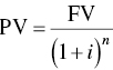
where i is now referred to as the discount rate. Thus, if the discount rate is 5% per year, we calculate the PV of $100 to be spent 12 years as follows:

Since the PV of money to be spent in the future declines with increasing interest rate and number of years into the future, the importance of accounting for the time at which money is spent or received is evident.
7.5 Calculating CF
A complete financial analysis requires the inclusion of CF. On a year‐by‐year basis, the CF from a manufacturing investment is determined through calculations of cash costs, total costs, and cost‐effectiveness.
Cash costs, those associated with operating and overhead, include raw materials (chemicals, catalysts, solvent, etc.) utilities (steam, electricity, natural gas, water, etc.), maintenance materials and labor, operations labor, technical support, startup costs, taxes and insurance, and administrative costs.
Total costs include the sum of cash costs as just defined and depreciated. Note that depreciation is not a cash cost and is used only to calculate income taxes. If the investment generates revenues or savings from which the total costs may be subtracted, the resulting amount is known as the “pretax earnings.” Income taxes (calculated on pretax earnings) are next subtracted to yield the after‐tax earnings. A year‐by‐year CF can then be determined by summing the four real CFs: investment, cash costs, revenues, and income taxes.
NPV is the sum of the PVs of a series of CFs:
where, CF0, CF1, CF2 represent CF in year 0, 1, 2, and so on, and the D terms are discount factor for the respective years.
In the context of pollution control, cost‐effectiveness is defined as the annualized cost of the control option divided by the annual emission reductions resulting from the control option. The following information is required to calculate the cost‐effectiveness of a proposed control option: (i) the capital cost of purchasing and installing the control equipment or making a process modification, (ii) the annual operating costs of the control option, and (iii) an estimate of the emissions before and after application of the control option.
The capital costs of purchasing the control option should be determined from actual vendor price quotes for each proposed control option. Installation costs should also be based on vendor price quotes. If vendor price quotes are unavailable, elements of the installation cost may be estimated (Vatavuk 2002). To illustrate cost‐effectiveness calculations, let us consider a facility that is a major source of NOx emissions.
7.5.1 Achieving a Responsible Balance
In the real worlds, taking socially desirable action for pollution prevention may not be in the best interest of an industry in the short run, since environmental protection costs money. The type of production, input used, technology employed, space used as well as plant size and the scale of production determine the nature and extent of pollution which, in turn, influence the abatement cost. Hence, the decisions of the profit maximizing private investor for implementation of pollution abatement measure are influenced by the benefit expected as a result of the investment required. On the other hand, the task of government planners and policy makers is to encourage industry to adopt modern production and pollution control technologies to provide a better environment for the society. In upgrading their facilities to meet the near antipollution regulations, industries turn for guidance to the principles of best available control technology (BACT).
7.6 From Pollution Control to Profitable Pollution Prevention
As companies incorporate pollution prevention approaches in their strategic planning, capital investment priorities, and process design decisions, it is vital that they understand both the quantitative and qualitative dimensions of assessing pollution prevention projects. These projects tend to reduce or eliminate costs that may not be captured in cursory financial analyses due to the way costs are categorized and allocated by conventional management accounting systems. Additionally, pollution prevention projects often have impacts on a broad range of issues, such as market share and public impact that are difficult to quantify but that can be of strategic importance. Identifying and analyzing all costs and less tangible items is an important step in an evaluation of the potential benefits of pollution prevention projects.
Pollution prevention can take many forms – from simple “housekeeping improvements,” which cost little to carry out, to installation of expensive capital equipment. Although many pollution prevention projects, such as material substitution or process redesign, do not require large outlays for purchase of equipment, they may require extensive qualitative assessments related to such issues as product quality or employee health and safety. The analytical tools described here are applicable to the assessment of most pollution prevention initiatives that fit under the umbrella of the capital budgeting process. Pollution prevention projects involving capital budgeting generally include
- new manufacturing equipment
- replacement equipment
- plant expansion and construction
Capital budgeting is a process of evaluating capital investment options based on a company's needs and analyzing the impact of an investment on a company's CF over time. Pollution prevention and other capital projects are justified by showing how the project will increase the company's earnings as well. Financial tools demonstrate the importance of the pollution investment on a life cycle or total cost basis in terms of revenue, expenses, and profits. Key concepts and factors used in capital budgeting are described next.
Life cycle costing (LCC): Also referred to as total cost accounting, this method analyzes the costs and benefits associated with a piece of equipment or a procedure over the entire time the equipment or procedure is to be used. LCC is also a tool to determine the most cost‐effective option among different competing alternatives to purchase, own, operate, maintain and, finally, dispose of an object or process, when each is equally appropriate to be implemented on technical grounds. For example, for a highway pavement, in addition to the initial construction cost, LCC takes into account all the user costs (e.g. reduced capacity at work zones), and agency costs related to future activities, including future periodic maintenance and rehabilitation. All the costs are usually discounted and total to a present‐day value known as NPV. This example can be generalized on any type of material, product, or system.
In order to perform a LCC scoping is critical, what aspects are to be included and what not? If the scope becomes too large, the tool may become impractical to use and of limited ability to help in decision‐making and consideration of alternatives; if the scope is too small, then the results may be skewed by the choice of factors considered such that the output becomes unreliable or partisan. LCC has a broader scope, including environmental costs. To help building and facility managers make sound decisions, the US Federal Energy Management Program provides guidance and resources on applying LCC that permits the cost‐effectiveness of energy and water efficiency investments to be evaluated. LCC can be conducted in two approaches: deterministic and probabilistic method.
Present value (PV): The importance of PV, or present worth, lies in the fact time is money. The preference between a dollar now and a dollar a year from now is driven by the fact that dollar in‐hand can earn interest. Mathematically, this relationship is shown earlier in Eq. (7.2), with an example on present and future values.
Comparative factors for financial analysis: The more common methods for comparing investment options all utilize the PV equation presented in Eq. (7.2). Generally, one of the following four factors is used:
- Payback period (PP): This factor measures how long it takes to return the initial investment capital. Conceptually, the project with the quickest return is the best investment.
- Internal ROR: This factor is also called return on investment or ROI. It is the interest rate that would produce a return on the invested capital equivalent to the project's return. For example, a pollution prevention project with an internal ROR of 20% would indicate that pursing the project would be equivalent to investing the money in a bank and receiving 20% interest.
- Benefits cost ratio: This factor is a ratio determined by taking the total PV of all financial benefits of a pollution prevention project and dividing by the total PV of all costs of the project. If the ratio is greater than 1.0, the benefits outweigh the costs and the project is economically worthwhile to undertake.
- Present value of net benefits: This factor shows the worth of a pollution prevention project as a PV sum. It is determined by calculating the PVs of all benefits, doing the same for all costs and subtracting the two totals. The new result would be an amount of money that would represent the tangible value of undertaking the project.
7.6.1 Life Cycle Costing
While firms can use any of these factors, the importance of the LCC (for total cost analysis) makes the PV of net benefits the preferred method. Additional details of LCC and TCA follows.
LCC tool and the total cost assessment (TCA) tool are introduced as concept overviews. Both tools can be used to establish economic criteria to justify pollution prevention projects. TCA is often used to describe the internal costs and savings, including environmental criteria. LCC includes all internal costs plus external costs incurred throughout the entire life cycle of a process, product, or activity.
LCC has been used for many years by both public and private sector. It associates economic criteria and societal (external) costs with pollution prevention opportunities. The purpose of LCC is to quantify a series of time varying costs for a given opportunity over an extended time horizon, and to represent these costs as a single value. These time varying costs usually include the following:
- Capital expenditures. Cost for large, infrequent investment with long economic lives (e.g. new structures, major renovation and equipment replacement).
- Nonrecurring operations and maintenance (O&M). Costs reflecting items that occur on a less frequent than annual basis that are not capital expenditures (e.g. repair or replacement of parts in a solvent distillation unit).
- Recurring O&M. Costs for items that occur on an annual or more frequent basis (e.g. oil and hydraulic fluid changes).
- Energy. All energy or power generation related costs. Although energy costs can be included as a recurring O&M cost, they are usually itemized because of their economic magnitude and sensitivity to both market prices and building utilization.
- Residual value. Costs reflecting the value of equipment at the end of the LCC analysis period. This considers the effects of depreciation and service improvements.
By considering all costs, a LCC analysis can quantify relationships that exist between cost categories. For example, certain types of capital improvements will reduce operations, maintenance, and energy costs while increasing the equipment's residual value at the end of the analysis period.
Societal (external) costs include those resulting from health and ecological damages, such as those related to unregulated emissions, wetland loss, or deforestation, can also be reflected in a LCC analysis either in a qualitative or in a quantitative manner. LCC includes the following cost components:
- Extraction of natural resources. The costs of extracting the materials for use and any direct or indirect environmental cost for the process.
- Production of raw materials. All of the costs of processing the raw materials.
- Making the basic components and products. The total cost of material fabrication and product manufacturing.
- Internal storage. The cost of packaging and storage of the product before it is shipped to distributors and/or retail stores.
- Distribution and retail storage. The cost of distributing the products to retail stores including transportation costs, and the cost of retail storage before purchase by the consumers.
- Product use. The cost of consumer use of the product. This could include any fuels, oils, maintenance, and repairs which must be made to the equipment.
- Product disposal or reuse and/or recycling. The costs of disposal or recycling of the product.
7.6.2 Total Cost Assessment
The TCA tool is especially interesting because it usually employs both economic and environmental criteria. As with the LCC analysis, the TCA study is usually focused on a particular process as it affects the bottom‐line costs to the user. Environmental criteria are not explicit, i.e. success is not measured by waste reduction or resource conservation, but by cost savings. However, since the purpose of TCA is to change accounting practices by including environmental costs, environmental goals are met through cost reductions.
Because of its focus on cost and cost effectiveness, TCA shares many of the features of LCC analysis by tracking DC, such as capital expenditures and O&M expenses/revenues. However, TCA also includes IC, liability costs, and less tangible benefits – subjects that are not customarily included in both economic and environmental goals, because of its private‐sector orientation, as well as other economic computation methods.
7.6.3 Economic Consideration Associated with Pollution Prevention
The greatest driving force behind any pollution prevention (P2) plan is the promise of economic opportunities and cost savings over long‐term. Pollution prevention has been recognized as one of the lowest‐cost options for waste/pollutant management. Hence, an understanding of the economics involved in P2 programs/options is important in making decisions at both the engineering and management levels. Every engineer should be able to exercise an economic evaluation of a proposed project. If the project cannot be justified economically after all factors – include those discussed earlier have been taken into account – it should obviously not be pursued. The earlier such a project is identified, the fewer resources will be wasted.
Before the true cost or profit of a P2 program can be evaluated, the factors contributing to the economics must be recognized. As discussed earlier, there are two traditional contributing factors (capital costs, and operating and maintenance costs), but there are also other important costs and benefits associated with P2 that need to be quantified if a meaningful economic analysis is going to be performed. The TCA aims to quantify not only the economic aspect of P2 but also the social costs associated with the process, product, or a service from cradle‐to‐grave (i.e. life cycle). The TCA attempts to quantify less tangible benefits such as the reduced risk derived from not using a hazardous substance. The future is certain to see more emphasis placed on the TCA approach in any P2 program. For example, a utility considering the option of converting from a gas‐fired boiler to coal‐firing is usually not concerned with the environmental effects and implications associated with such activities as mining, transporting, and storing the coal prior to its usage as an energy feedstock. Pollution prevention approaches will become more aware of this kind of need.
7.7 Resource Recovery and Reuse
A critical element of an interim strategy is enhanced recovery. This can be approached from two directions: reuse of products and recycling of materials. Reuse of products includes return, reconditioning, and remanufacturing. The energy required for reuse and recycling is one of the key factors determining recoverability of a product. The closer the recovered product is to the form it needs to be in for recycling, the less energy is required to make that transformation. From the standpoint of economic development it is worth pointing out that the reconditioning or remanufacturing cycle is relative; it requires roughly half the energy and twice the labor per physical unit of output.
Recycling materials means closing the loop between the supply of postconsumer waste and the demand for resources for production. Recycling of materials will be the business of the Zero Emissions engineer; reuse of products will also involve the Zero Emissions engineer, but will have lots of front‐end work from another professional, the concurrent engineer. Concurrent engineering, which incorporates aspects of industrial engineering, product design, and product manufacturing, is an integrated approach that seeks to optimize materials, assembly, and factory operation. These engineers examine the broader context of a product, including technology for managing the environmental impacts of its transport, intended use, recyclability, and disposal, as well as the environmental consequences of the extraction of the raw material used in its production.
The ultimate fate of all materials is thus dissipation, being discarded, or recycling and recovery. With 94% of materials extracted from the environment being converted to wastes, current levels of recovery are clearly not sufficient. Recovery of materials from wastes will reduce the extent of resource extraction (but will not slow the speed of material flows through the economy). Aluminum and lead are two resources currently being heavily recycled, but evidence shows that there is potential for a lot more resources to be recovered from wastes.
Sherwood plots are diagrams that permit the graphic comparison of concentrations of materials in nature against their commodity cost. The sample plot (see Figure 1.7) shows that the price for a commodity depends on its concentration in nature before extraction and refining. In a similar plot (see Figure 1.8) for concentrations of materials in wastes, it again shows a consistent line.
Together, the Sherwood plots demonstrate the recovery potential of materials. The elements plotted above the line shown in Figure 1.7 should be vigorously recycled because they are present in individual by‐products in relatively high concentrations. Lead, zinc, copper, nickel, mercury, arsenic, silver, selenium, antimony, and thallium are more economical to recover from waste than from nature. Extensive waste trading could significantly reduce the quantity of material requiring disposal because resource extraction uses from wastes, not virgin feedstocks (Allen and Rosselot 1997).
7.8 Profitable Pollution Prevention in the Metal‐Finishing Industry
Surface finishing of metal products is a major manufacturing operation performed in thousands of production shops to provide weather‐resistant, wear‐resistant, and aesthetically pleasing finishes for thousands of manufactured products.1 Surface‐finishing technology involves direct atom‐to‐atom bonding between a base material (such as steel, aluminum, brass, or plastics) and a metal or organic surface top coating that provides the desired material performance and appearance properties. Surface pretreatment is crucial for proper performance and durability of the produced part. Cleaning and oxide removal is critical, so pretreatment processes usually involve many tanks with various purposes. Multistep surface preparation processes are generally employed to remove oils, soiling and dirty materials, old coatings, corrosion products, residual cutting fluids, brazing residuals, pickling acid residuals, cleaner residuals, etc. The surface preparation process removes contaminants, preserves the cleaned surface, and/or modifies the surface for the next coating. After the finishing process, the parts require rinsing/cleaning to remove residual plating solution. These baths, both plating and cleaning, ultimately are exhausted because of depletion of strength or buildup of impurities and, as a result, become major waste streams (Burckle and Ferguson 2005; USEPA 2001).
In the past, pollution control in the metal‐finishing industry has been achieved primarily through end‐of‐pipe treatment. Facilities added waste treatment systems as a final process step to meet regulatory discharge limits to municipal sewers or as direct dischargers. This approach results in the production of residual sludges contaminated with heavy metals that require appropriate pretreatment for environmentally safe disposal (the so‐called “Hammer Provisions” of the Resource Conservation and Recovery Act that apply to hazardous waste disposal in the United States). In the mid‐1980s, various facilities began integrating “pollution prevention” into their operations to reduce the amount of wastewater generated and treated. However, the speed of adoption has been relatively slow, most noticeably in smaller facilities (USEPA 1982, 1985).
The most logical and efficient approach to effectively achieve environmental protection is by preventing pollution. Prevention is achieved using techniques that reduce, eliminate, or recycle/reuse waste materials so that the generation of waste is eliminated, avoiding the need for waste disposal, and wastes that are generated are handled responsibly, either through recovery and recycling to displace other material needs and/or to conserve energy, or minimized and made safe for disposal into the environment. The metal‐finishing industry began to apply pollution prevention principles to reduce process waste emissions in the mid‐1980s, but there were no public statistics generated of the impact on pollution avoided or economic benefit accrued. In discussing the progress of domestic metal‐finishing industry in transitioning to operations based upon pollution prevention, we begin by describing the National Metal Finishing Strategic Goals Program (SGP) initiated by the US Environmental Protection Agency (USEPA) in 1998 in cooperation with industry and public interest stakeholders (USEPA 1998, 2001).
7.8.1 National Metal Finishing Strategic Goals Program
This was the first nationwide program initiated by the USEPA to build voluntary participation in a compliance program by providing incentives in return for a real commitment to reducing pollution to levels below those required for compliance. The SGP was created to address environmental problems and institutional barriers to achieving compliance in a number of industries. It was designed to provide a working relation that facilitates and encourages companies to go beyond environmental compliance to pollution prevention–based operations. SGP member companies were offered incentives, resources, and a means for removing regulatory and policy barriers as they work to achieve specific environmental goals.
The SGP program brought together stakeholders to identify important issues, conduct demonstration projects, and develop consensus policy recommendations that offered opportunities for reducing pollution. The stakeholders included industry, labor, environmental groups, state and local government, and other federal agencies. The metal‐finishing industry was represented by the National Association of Metal Finishers, American Electroplaters and Surface Finishers Society, Metal Finishing Suppliers Association, and Surface Finishing Industry Council. Through the SGP (USEPA 2001), the participants worked together to improve environmental performance and the bottom line.
Participation required top management commitment to the implementation and maintenance of an approved Environmental Management System (EMS). The EMS has caused management to take careful note of the true costs of pollution and institute policies and procedures to eliminate this waste at its source (USEPA 2003a). The results of these efforts have provided the first large‐scale quantification of the power of pollution prevention for achieving significant reductions in pollution and the resulting economic benefits in the metal‐finishing industry. The SGP program was designed to help a metal‐finishing company achieve its goals – both environmental and economic. A wide variety of state and local SGP resources (USEPA 2001) were available to provide a company with the tools need to get the job done. These include the following:
- Free, non‐regulatory environmental audits
- Funding for environmental technologies
- On‐site technical assistance in (evaluation and planning) achieving compliance and improving pollution prevention, safety, and health measures
- Free assistance from interns to help fill out the SGP data worksheets
- Free workshops on energy, water, and waste reduction
- Regulatory flexibility
- EMS training
- Public recognition
All parties benefited from the use of these tools. A few of the advantages listed in the project report are listed here.
- Companies received the incentives and resources needed to take the risk of going beyond compliance requirements.
- As the participating companies employ less‐polluting technologies, waste is reduced, less pollution is discharged to the environment, and the plant saves money, becoming more cost efficient and competitive.
- As the results demonstrated in the participating plants are employed by other plants to reduce pollution and improve competitiveness, the practices of pollution prevention are spread throughout the industry.
- The industry as a whole benefits from the positive action of SGP member companies.
- As the metal‐finishing industry becomes increasingly more self‐regulated, government regulators – from the EPA to the local publicly owned treatment works – save time and money.
The SGP has seven environmental performance goals (USEPA 2001) that form the core of the program (see Table 7.1). Through the end of 2000, many participants had already made significant progress toward meeting the goals, which translated into real environmental gains:
- 380 million gal of water conservation
- 120 million lb of hazardous waste not sent to landfills
- 665 000 lb of organic chemicals not released to the environment.
A comparison of the reductions achieved through 2000 and 2003 shows continuing and significant improvements in pollution prevention. This continued progress of the participants is a positive indicator of the benefits of a program driven by the employment of the EMS. The SGP participants were provided free, non‐regulatory environmental audits and access to technical support in achieving compliance and improving pollution prevention. Data like this readily demonstrates the power of the EMS management tool to reduce pollution. But to see how this progress was achieved, we must examine the role of pollution prevention (P2) technologies in enabling the reductions.
Table 7.1 Progress towards SGP goals.
| SGP goal | Average achievement by SGP metal finishers (over all projects) | |
| 2000 | 2003 | |
| 1) 50% reduction in water usage 2) 25% reduction in energy use 3) 90% reduction in organic toxic release inventory (TRI) releases 4) 50% reduction in metals released to water and air 5) 50% reduction in land disposal of hazardous sludge 6) 98% metals utilization 7) Reduction in human exposure to toxic materials in the facility and surrounding community |
41% reduction 14% reduction 77% reduction 58% reduction 36% reduction 17% utilization factor 51% of activities accomplished |
56% reduction 41% reduction 84% reduction 65% reduction 48% reduction 64% utilization factor 85% of activities accomplished |
7.8.2 The Role of Pollution Prevention Technologies
7.8.2.1 Moving Toward the Zero Discharge Goal
A highly desirable “state” for environmental protection would be Zero Discharge of pollutants to the air, water, and land. Today, this is a goal not yet realized. However, “approaching” Zero Discharge has been found to be realistic, as demonstrated by the continual improvement in environmental performance achieved in the SGP for the metal‐finishing sector. Approaching Zero Discharge can be defined as reducing wastes emitted from a process by a significant amount, with significant reduction ranging from a low defined by the regulatory standard and the high defined by the technology employed.
There are two key elements to achieving movement toward the state of Zero Discharge – implementation of an EMS and deployment of certain technologies based upon pollution prevention. The framework of an EMS is the management tool that provides a state of “continuous assessment and compliance of plant operations,” while P2 technologies provide the technological tools needed to achieve significant improvements in performance and reductions in generation of waste.
7.8.2.2 Planning and Implementation
As part of the planning phase, a compliance assessment of a participating plant is necessary to establish a baseline against which progress and savings in incremental costs can be measured. The goal of the plant assessment is to identify the root causes of the most significant problems, to identify areas in which P2 options could save the most money, and to assign priorities to address the most significant problems. The plant assessment must include an inventory of all chemicals, wastes, bath chemistries; the overall plant layout; and a site inspection. Once the problems are identified and prioritized, various solutions can be proposed and the effects of their deployment evaluated. A comprehensive plan addresses housekeeping and maintenance issues in order to sustain any P2 efforts and also to establish good standard practice.
This planning approach is most efficiently implemented through an EMS. In addition, the imperatives of “total quality management” apply. Management must buy into the process and be willing to provide the necessary resources to achieve success. Experience has shown that often the best solutions come from those working most closely to the problem. It is important that employees be included in the improvement program and kept well informed so that they will become stakeholders in the process.
Implementation through an EMS has several advantages. First it is more effective because it provides a tool for involving management through its provision for continuous improvement in both environmental performance and worker health and safety. Second, it provides a mechanism to integrate process and product quality issues that influence reduction of waste and the improvement of productivity and profitability. The review of these considerations should be incorporated into the process and reviewed over time as a pathway for identifying future opportunities and establishing priorities. This process leads to the identification of the power of pollution prevention technologies to achieve these savings offered by waste reduction. The Agency provides an EMS template tool (USEPA 2004; Stander and Theodore 2008) to assist those who are interested.
Many of the same elements that must be defined for the compliance assessment are also needed to establish an EMS. Certification under the ISO 14001 – an EMS that is standardized worldwide – is being increasingly required of those companies engaged in the manufacture of products for export, including components in the supply chain of such products. Also the EPA offers Compliance Incentives – “policies and programs that eliminate, reduce, or waive penalties under certain conditions for business, industry, and government facilities which voluntarily discover, promptly disclose, and expeditiously correct environmental problems” and is including a requirement for the implementation of EMSs in settlements. Information about these incentives, programs, and the environmental benefits achieved by such programs may be found on the Internet (http://www.epa.gov/compliance/incentives/index.html).
7.8.2.3 Practicing Pollution Prevention
Technologies based on the precept of Pollution Prevention serve to eliminate the generation of wastes or to reduce the disposal of wastes through recycle/reuse. Pollution in the metal‐finishing industry is basically the discharge of some unwanted form of material or other resource (energy, labor, time, etc.). Loss of these resources equates to the loss of profit and economic productivity. It stands to reason that the more of a resource used above the minimum required by the process, the more this incremental use (read: “waste”) adds to the “unnecessary” component of the total costs of the operation. In the case of water use, for example, this unnecessary cost is not just the cost of the excess water wasted. The cost of this waste is magnified by the costs for its overall management for treatment and disposal, including the capital and operating costs for moving the excess water through the process, its cleaning, and the disposal of the treated water and any residual wastes. The treatment and disposal costs are usually more costly than the initial raw material. Often these costs (process operations and compliance costs) are not tracked by a company because the accounting process used is inadequate to perform such tracking.
Companies participating in the SGP have found significant cost savings by implementing P2 practices (USEPA 2001). Significant cost savings result in improved economic efficiency and an improved bottom line on the balance sheet, making the operation more competitive. Other advantages include the protection of employees, reduction of liabilities, and, at the same time, enhancement of the company's business image.
Success in achieving the goals of the SGP for the metal‐finishing sector has been attributed largely to the employment of pollution prevention techniques. A principal purpose of the program was to demonstrate the attractive environmental and economic advantages offered by P2‐based approaches to waste reduction. The outcome anticipated was to “stimulate a keen awareness and appreciation” of these extremely valuable tools so that they would be adopted into everyday practice on a sector‐wide basis. In addition, the adoption of an EMS and integration into company operations ensures continued improvements (both in environmental performance and in cost savings) within the entire fabric of the participating companies.
There are many approaches to reduce pollution in various unit processes that were investigated and documented by USEPA sponsored research in the 1980s, including housekeeping and maintenance methods and management of process chemicals and rinse water. These methods are described in the EPA Capsule Report entitled Approaching Zero Discharge in Surface Finishing (USEPA 2000) and the training course document entitled P2 Concepts & Practices for Metal Plating & Finishing (AEFS, American Electroplaters and Surface Finishers Society). These learning aids address a number of process design areas such as those listed in Table 7.2.
Transitions of manufacturing operations to P2‐based systems have been demonstrated using a range of technology options from relatively simple improvements in existing process technology to more sophisticated approaches based upon significant process changes. There are numerous examples of the power of pollution prevention technologies, ranging from relatively simple improvements of water management to more sophisticated recovery processes, as documented in the results of the SGP and other programs.
Table 7.2 Pollution prevention technologies for surface finishers.
| To improve in these operations | Employ these technologies and practices |
Extend bath life
|
|
Reduce water consumption
|
|
Minimize waste
|
|
Reduce the use of hazardous chemicals
|
|
7.8.2.4 Case Study: An Emerging Profitable Pollution Prevention Technology
The USEPA recently completed a study of the proprietary Picklex process. Picklex® is a “‘non‐polluting’ pretreatment/conversion coat which replaces chromate conversion coating and zinc & iron phosphatizing in powder coating, paint and other organic finish applications” (Ferguson and Monzyk 2003; Ferguson et al. 2001).
Description
Metal pretreatment is crucial for cleaning and oxide removal to obtain proper performance and durability of the produced part, and it usually involves many tanks with various purposes. For example, aluminum anodizing may require eight pretreatment tanks; in conventional chromate conversion coating, there are twelve stages, while conventional zinc phosphatizing requires six. All of these baths contain heavy metals and must be dumped periodically.
The volume of hazardous/toxic waste streams produced from metal surface–finishing operations is significant (USEPA 1995a). The elimination of any of the surface‐processing steps is beneficial to the manufacturing process because it reduces processing costs, waste production, and energy consumption. Strong acids used in the pretreatment of metals pose a great health and safety risk to workers. With this in mind, a no‐waste or waste‐reducing surface‐finishing agent designed to lower processing costs for metal‐finishing operations would be of great benefit.
The Picklex process (a proprietary process) is one such alternative to conventional metal surface pretreatment that offers significant reductions in waste generation. The process was developed by International Chemical Products, Inc. with assistance from the USEPA. The Picklex process works in a completely different way than conventional processes. It incorporates the corrosion products from the metal surface into the protective coating that is applied to that same metal surface. This new P2 approach “thinks outside the box” by solving the common environmental problem of metal buildup in the processing tanks while forming a protective surface coating on the work piece. A two‐phase program was undertaken to evaluate the ability of Picklex to perform technically and economically as a pollution prevention–based replacement for conventional metal pretreatment or pretreatment/conversion coat in finishing operations. The goal was to demonstrate its potential to eliminate or significantly reduce the amount of hazardous and toxic chemicals consumed and the amount of pollution generated while maintaining equal or better product performance properties.
A broad laboratory evaluation of Picklex was undertaken in which full multistep, bench‐scale, batch operation tests using side‐by‐side test lines of seven conventional processes and of Picklex were performed. The results of the laboratory tests were quite favorable, and field tests (Ferguson and Monzyk 2003) were conducted to evaluate in‐plant performance in side‐by‐side tests with conventional preparation technologies. Only the most promising applications – the replacing of chromate conversion coating and zinc phosphatizing – were taken to field evaluation. In these focused field tests, Picklex was used to prepare aluminum and steel substrates for powder coating only. Although the testing scope was narrowed, it was more detailed. A total of 41 different combinations of substrate, degreaser, pretreatment, conversion coat, and powder coat were tested in the field evaluation. Only uncontaminated panels and components, without corrosion products, were used. The results for all test cases demonstrated that the quality of the final product was equal in all respects to conventional practice. Product quality was targeted as the single most important acceptance criterion within all the comprehensive results, because if the final product quality was not acceptable, the pollution reductions would not matter. The field test results replicated those obtained earlier, indicating that the lab testing may be used to accurately predict results achievable in practice.
7.8.2.5 Environmental Benefit
Two commercial processes, chromate conversion coating and zinc phosphatizing, were employed in the field tests as the experimental control baseline (Figures 7.3 and 7.4, respectively). Metal buildup in these conventional processes ruined the baths, and the baths had to be dumped. In the metal‐finishing sector, the discarding of such metal‐containing waste streams is a major contributor to pollution. The Picklex chemical used in the process tank is used up on the product; however, with filtering, the bath does not become contaminated. As a result, it is not necessary to dump the bath to control impurity buildup, and the chemical make‐up is simply added to the bath as needed. This process was demonstrated to have a strong potential as a leading technology for pollution prevention in surface preparation operations.
As can be seen in the comparison of the conventional practices to this emerging technology, the Picklex process eliminates up to eleven steps in metal‐finishing processes. The reductions of waste at the source were very significant. These reductions were accomplished by the elimination of the hexavalent chromium tank and subsequent rinsing operations; the elimination of the acid baths used for etching and cleaning along with subsequent rinsing operations; the elimination of the zinc phosphatizing baths and subsequent rinsing operations; and the elimination of the deoxidizing bath and subsequent rinses. All of the steps eliminated are steps that emit pollution. In addition, the Picklex process significantly reduces the pollution from the remaining steps. It does this while providing the same high‐quality finish and wear resistant capabilities as the conventional processes.
Figure 7.3 Comparison of Picklex to conventional chromate conversion coating.
Figure 7.4 Comparison of Picklex to conventional zinc phosphatizing.
Although normally the Picklex bath does not need to be dumped, but, as part of the study, the bath was evaluated for waste treatment issues in the event of a spill or accidental contamination. Fresh, spent, and impurity‐spiked spent Picklex samples were treated using the conventional pH 9 precipitation industrial wastewater treatment method to produce samples for a waste disposal assessment for Picklex. The waste solids were assessed for toxic leachability. The treated water supernatants for discharge were also examined and found as most likely dischargeable. Waste treatment may not be frequent or necessary in many processes. Actual discharge limits from industrial waste treatment plant operations are site‐specific and are determined on a case‐by‐case basis with local, state (and federal only where necessary) regulatory agencies. Hence, no exact classification of these potential waste solutions is possible until a specific location is known. All leachates are passed with respect to the applicable federal regulations (USEPA 1995b). Therefore, Picklex does not appear to present unusual waste treatment issues.
7.8.2.6 Economic Benefit
A cost comparison was made for two most promising processes – replacing chromate conversion coating and zinc phosphatizing. These were chosen based on the potential cost savings that industry could achieve. There would appear to be a significant economic incentive to migrate existing practice to this new technology, based on the significant capital and annual operating costs that is projected for the Picklex technology, summarized in Table 7.3. In fact, a new shop adopting the process in place of chromate conversion coat would save capital costs of $254 000, with the reduction of the process from 12 to 1 tank (Figure 7.3). For zinc phosphatizing on steel, the savings is estimated to be $230 000.
Table 7.3 Potential cost savings.
Source: From Ferguson and Wilmoth (2000) and Ferguson et al. (2001).
| Cost type | Savings of Picklex over conventional process | |
| Chromate conversion coat on aluminum ($) | Zinc phosphatizing on steel ($) | |
| Capital cost savings | 254 000 | 230 000 |
| Annual operating cost savings | 46 000 | 32 000 |
7.8.2.7 Technology Transferability
The Picklex technology is very robust and flexible (Ferguson and Monzyk 2003). It is applicable from the very large to very small operations. It can be used in a new installation, in a retrofit for process modernization, or as a drop in replacement for any existing facility. Picklex can be applied by dipping the part in tanks or by spraying or brushing. Cost savings are very significant and are a function of the size of the facility and the number of processing lines that are required. Transferability is enhanced by the prospective significance of the overall facility cost savings and productivity improvements offered.
7.8.3 Value‐Added Chemicals from Pulp Mill Waste Gases
Methanol, formed during the pulping of wood and is contaminated with reduced sulfur compounds and terpenes, is the largest single source of VOC emissions from kraft pulp mills, accounting for 70–80% of total emissions. The Cluster Rule (Cluster Rule Regulation: 40CFR Part 63 1998) limits methanol emissions for all pulp mills in the United States. Canada faces similar legislation (Das 1997, 1999a, b; Das and Houtman 2004; Das and Jain 2001).
Methanol emissions can be reduced by collecting condensate streams from the digesters, evaporators, and other sources in the mill. The collected condensate streams can then be steam‐stripped to concentrate the methanol for incineration. A few mills are “hard‐piped” to send this methanol‐laden stream to bio‐treatment plant, thus avoiding incineration.
Stripper overhead gas (SOG) contains roughly equal part of methanol and water (40–50 wt%) and roughly equal parts of TRS and terpenes (1–5 wt%).
In the United States, the SOG is likely to be burned in an incinerator, kiln, or boiler. Recently, some mills have found it advantageous to rectify the SOG to about 80% methanol and collect it as a liquid, which has a higher fuel value. With this concentrated (70–80%) methanol stream available, plants can cut down on the amount of natural gas that must be bought.
A process has been developed at Georgia‐Pacific that converts the methanol and TRS (mostly mercaptans) in the rectified SOG into formaldehyde. Based on work by Wachs (1999a, b), this patented catalytic process (Burgess et al. 2002) has achieved commercially viable yields of formaldehyde (70–80%) from a typical pulp mill SOG feedstock containing methanol, water, and TRS compounds.
The conversion of methanol and TRS to formaldehyde presents kraft mills with a more profitable alternative for SOG than incinerating the gas as a fuel. The formaldehyde produced can be used by resin manufacturers to produce thermosetting resins commonly used in plywood and other structural panels. A typical pulp mill of 2000 air‐dried tons per day (ADTPD) output may achieve a payout of 2–4 years, depending on the price of methanol and local economics.
Table 7.4 Annualized income, costs, and earnings 2000 ADTPD mill, 14 lb methanol/T SOG.
Source: From Burgess et al. (2002).
| Income 15 000 000 lb/year formaldehyde (50%) at $0.06/lb, FOB mill | $900 000 |
| Operating cost | |
| Direct labor | $110 000 |
| Utilities | $25 000 |
| Methanol in feed at $2.25/MMBTU fuel value | $260 000 |
| Misc., catalyst, supplies, etc. | $70 000 |
| Total operating cost | $465 000 |
| Gross margin | $435 000 |
| Depreciation | $210 000 |
| Earning before tax | $225 000 |
| Credit for steam generated (depending on the mill's steam balance) | $95 000 |
| Credit for terpene recovered and sold | $110 000 |
| Credit for SO2 recycled | $45 000 |
| Total by‐product credits | $250 000 |
| Total earnings, including by‐product credits | $475 000 |
The process also produces two levels of low‐pressure stream, 60 and 70 psig, usable within a paper mill, by reducing most of the methanol to formaldehyde, rather than CO2. The reduction in CO2 emissions is about 80–85% of the amount otherwise generated by incineration or by the bio‐treatment plant. For a 2000 APTDP mill, this equates to 28 T/Y of CO2 emissions that are avoided.
A typical itemization of income, costs, and earnings is given in Table 7.4. For a 2000 ADTPD mill, a payout of 3–4 years is calculated based on formaldehyde prices of $0.06/lb (50%) basis. This assumes a customer‐shipping radius of 500 miles from the mill producing the formaldehyde. A heat value credit to the mill is included (equivalent of natural gas fuel) for the methanol that would otherwise have been incinerated and used to generate steam via heat recovery exchangers.
7.8.4 Recovery and Control of Sulfur Emissions
Sulfur is often considered one of the four basic raw materials in the chemical industry. It can be recovered as a by‐product from sulfur removal and recovery processes (Kirk and Othmer 2004). Historically, sulfur recovery processes focus on the removal and conversion of hydrogen sulfide (H2S) and sulfur dioxide (SO2) to elemental sulfur, as these species represent significant emission from pulping process. Various processes for the removal of SO2 in the combustion gases are available. Direct catalytic oxidation of SO2 to SO3, and subsequent absorption of SO3 in water to produce sulfuric acid, is an alternative method (Paik and Chung 1996). Total mill TRS emissions of 10–20% are contributed by vent streams from brownstock washers, foam tanks, black‐liquor filters, oxidation tanks, and storage tanks that are not typically collected in the noncondensable gas system (Pinkerton 1999). The emissions from these sources can be collected and combusted for energy recovery, reducing the atmospheric emissions of TRS and VOCs.
7.8.4.1 Freshwater Use Reduction and Chemical Recovery and Reuse Save Million at Pulp Mill
Effluent Discharges
Before pulp mill effluents can be released to the environment they must be treated. Primary treatment involves the use of settling ponds or tanks in which suspended solids settle out of the liquid effluent. Solids can be composted and spread on land, converted to other useful products, or incinerated. Secondary effluent treatment includes oxidation and aeration in shallow basins having wide areas or in smaller areas using mechanical agitators and spargers to oxygenate fluids before release. Biological filter systems can be used to remove organic compounds and heavy metals, and often the process can be accelerated by adding nutrients and by using oxygen rather than air. In some areas, natural wetland systems have been designed to achieve this. Other means of treatment include lime coagulation and the elevation of pH to precipitate organic color bodies as calcium lignates. Once precipitated, the sludge is dewatered and incinerated to destroy organics.
It has been reported by NCASI that there was a 30% reduction in effluent flow from mills between 1975 and 1988. During the same period, final effluent 5‐day BOD and TSS decreased by 75 and 45% (NCASI 1991). Data for 1975, 1985, and 1988 are presented in Table 7.5. These reductions will continue as pulp and paper mills implement the so‐called best management plans (BMPs) required by the Cluster Rule. BMPs will require better management of process losses and spills and are expected to reduce effluent discharges. For example, in roughly 10 years, Simpson Tacoma kraft mill reduced its freshwater consumption by approximately 50% through various pollution prevention methods (K. Schumacher and M. Mammenga, personal communication; USEPA 1992a, b).
Table 7.5 Effluent discharges from pulp and paper mills.
Source: From Das (1997).
| 1975 | 1985 | 1995 | |
| Effluent flow (gal/T) | 22 800 | 17 200 | 16 000 |
| BOD (lb/T) | 18.0 | 4.8 | 4.4 |
| TSS (lb/T) | 13.0 | 8.3 | 7.1 |
Simpson Tacoma now uses about 18 million gal of freshwater per day (mgd) vs. 32 mgd in 1990s. This reduction in freshwater usage saves about $1.92 million/year (350/MG, city of Tacoma charges per average fixed and variable cost). The plant also saves money through reducing sodium hydroxide (NaOH) losses to sewers and to product fiber, by stopping overflowing weak washing dilute NaOH solution and through recycling processed water. Otherwise, NaOH would be needed to the process to make up for soda (sodium) lost. The saving is about 3.4 million/year (based on $375/T of NaOH and 25 T of NaOH saving per day). Simpson also saves $0.18 million/year by reducing losses of black liquor sulfur to sewer and stack (K. Schumacher and M. Mammenga, personal communication).
Other firms save water by installing savealls (devices which separate fiber from process water), heat exchangers, and other equipment which permit more reuse of process water. Internal water cleaning systems make it possible to substitute filtered white water for clean water. Separating process cooling and clean water is often necessary to achieve balance in operations and water use.
7.8.4.2 Brine Concentrator for Recycling Wastewater
Brine concentrators are vapor compression evaporator systems that produce distilled water and a very small salt concentrate stream. These are ideal for water recycling because the concentrate stream is so low that wastewater can be treated economically with a very high recovery and with no liquid discharge (Dalan 2005).
To comply with the regulations, both new and existing power plants that were using river water had to recycle their water wastes. Although vapor compression was not new to industry as an energy source, the technological fit with power plants was a natural because it allowed these facilities to use electricity they were generating as the source of the mechanical energy needed in recycling water.
Federal law was not the only factor prompting industry to turn to the use of brine concentrators for recycling wastewater. All over the country, there were local siting regulations, as well. Thus, with the advent of the private power industry in the early 1990s, entrepreneurs turned to Zero Discharge water systems, which allowed them to use sites with a limited water supply, far away from discharge points. Similarly, the move to clean‐burning natural gas diminished the importance of locating power plants near sources of fuel or water.
As of 2004, there were approximately 60 brine concentrators in the Unites States. They are sold as package plants, designed and constructed with energy conservation principles. All the original units were at coal‐fired power plants, but as metal smelters, manufacturers of chemicals and semiconductors, and other enterprises began to recognize the need to eliminate water discharges, the use of brine concentration has spread.
7.8.4.3 Economics of Brine Concentrator Systems
Based on the parametric cost information on brine concentrator systems, we will now overview some economic aspects of these systems.
Brine concentrators, and by extension, integrated zero liquid discharge systems, only make sense in grassroots facilities only when
- there is a shortage of surface or well water
- the facility needs water to operate
- there is no water discharge option, such as a source of potable water or a river
- a discharge permit is unobtainable
Zero Liquid Discharge takes away the siting constraint; that is, it is no longer necessary to locate the plant near a large usable water source or suitable discharge point. The economic advantage of such an effect is hard to generalize, being very specific to the actual circumstance.
The NPV of a Zero Discharge facility is negative. Dalan and Rosain (1992) found that a 265 gpm brine concentrator had operating costs of $8.94/1000 gal of water treated (total of $1 252 600/year), while the avoided cost of extra demineralizer regeneration chemicals was $216 000/year. The avoided cost amounts to 1.54/1000 gal. Since any dollar amount here is an operating expense, the CF is negative.
Table 7.6 Operating cost breakdown for a 265 gpm system resulting in a cost of $9.62/1000 gal of feed.
Source: From Dalan and Rosain (1992), updated by Dalan (2005).
| Item | Consumption | Unit cost ($) | Annual cost ($) |
| Operating labor | 1 mhr (maximum hourly rate)/h | 50/mhr | 438 000 |
| Maintenance (labor) | 2 mhr/h | 50/mhr | 87 600 |
| Maintenance (materials, including spare parts) | 80 000 | ||
| Electricity | 1 617 kWh | 0.05/kWh | 707 000 |
| Chemicals | |||
| Sulfuric acid | 293 lb/day | 0.06/lb | 6 416 |
| Polymers | 40 lb/day | 1.50/lb | 21 900 |
| Total chemicals | 28 316 | ||
| Total annual operating cost | 1 340 916 | ||
| $/1000 gal of feed | 9.62 |
A typical specific operating expense is in the $5–7/1000 gal treated range. In this estimate is the price of electricity at a retail price of 0.05/kWh. In grassroots power plant planning, the electricity is many times considered a parasitic load on the power plant (electricity needed to produce the power). In this accounting method, the cost of electricity is zero. The elimination of electricity as an operating cost brings the total treatment cost down to the $2–3/1000 gal range. The typical energy load for a brine concentrator is 100 kWh/1000 gal of water produced.
The determination of water economics is very geography specific. For example, in western Washington, water and sewer bills typically are in the $1–2/1000 gal range, whereas in eastern Washington, water costs more, if indeed it is economically available.
For non‐power plant applications, local high prices for electricity can be overcome by seeking out alternate energy sources. Compressors (the majority energy user) in brine concentrator plants have been installed that are steam driven or natural gas (via a natural gas engine) driven. Table 7.6 presents breakdown of typical operating costs (Dalan 2005; Haussman and Rosain 1996).
For existing facilities, installing a Zero Discharge plant makes sense when
- the discharge permit conditions change, with the result that the existing facility can no longer be operated economically
- the cost of water rights plus treatment fees exceed the operating costs of a Zero Discharge facility
This last point is illustrated by a mini‐case study.
7.9 Use of Treated Municipal Wastewater as Power Plant Cooling System Makeup Water: Tertiary Treatment vs. Expanded Chemical Regimen for Recirculating Water Quality Management
7.9.1 Introduction
Every day, water‐cooled thermoelectric power plants in the United States withdraw from 60 billion to 170 billion gal of freshwater from rivers, lakes, streams, and aquifers, and consumes from 2.8 billion to 5.9 billion gal of that water. Freshwater withdrawals for cooling in thermoelectric power production account for about 40% of all withdrawals, essentially the same amount as withdrawals for agricultural irrigation, as documented by the U.S. Geological Survey. Sustained droughts nationwide underscore the critical need to think about using treated municipal wastewater (MWW) for use in cooling in electric power generation. It needs a great deal of water for electric power production, to condense stream in the power plant stream cycle. Air cooling is possible, but it is more costly and less efficient. Water will continue to be the preferred coolant for new thermoelectric power plants (Dzombak 2013).
Motivation for the project: Increase in demand for electricity brings with it an increase in water needed for cooling. The cooling of thermoelectric power plants accounts for 41% of all freshwater withdrawal in the United States, i.e. approximately the same amount of water as is withdrawn for agricultural irrigation. Some areas of the United States have little or no freshwater available for use. Alternative sources of water are needed for new electric power production. The U.S. Department of Energy has been conducting and sponsoring research to investigate the feasibility and costs of using alternative sources of water for power plant cooling, especially in recirculating cooling systems which are required for most new power production in the United States.
Goals and highlights of the project: Treated MWW is a common, widely available alternative source of cooling water for thermoelectric power plants across the United States, as determined in a predecessor DOE project (2006–2009) by the project team. However, the biodegradable organic matter, ammonia–nitrogen, carbonate, and phosphates in the treated wastewater pose challenges with respect to enhanced biofouling, corrosion, and scaling, respectively. The overall objective of this study was to evaluate the benefits and LCC of implementing tertiary treatment of secondary treated MWW prior to use in recirculating cooling systems.
The study comprised bench‐and pilot‐scale experimental studies with three different tertiary treated MWWs, and LCC and environmental analyses of various tertiary treatment schemes. Sustainability factors and metrics for reuse of treated wastewater in power plant cooling systems were also evaluated. The three tertiary treated wastewaters studied were secondary treated MWW subjected to acid addition for pH control (MWW_pH); secondary treated MWW subjected to nitrification and sand filtration (MWW_SF); and secondary treated MWW subjected to nitrification, sand filtration, and GAC adsorption (MWW_NFG).
Tertiary treatment was determined to be essential to achieve appropriate corrosion, scaling, and biofouling control for use of secondary treated MWW in power plant cooling systems. The ability to control scaling, in particular, was found to be significantly enhanced with tertiary treated wastewater compared to secondary treated wastewater. MWW_pH treated water (adjustment to pH 7.8) was effective in reducing scale formation, but it increased corrosion and the amount of biocide required to achieve appropriate biofouling control. Corrosion could be adequately controlled with tolytriazole addition (4–5 ppm TTA), however, which was the case for all of the tertiary treated waters. For MWW_NF treated water, the removal of ammonia by nitrification helped to reduce the corrosivity and biocide demand. Additional GAC adsorption treatment, MWW_NFG, yielded no net benefit. For all of the tertiary treatments, biofouling control was achievable, and most effectively with preformed monochloramine (2–3 ppm) in comparison with NaOCl and ClO2.
LCC analyses were performed for the tertiary treatment systems studied experimentally and for several other treatment options. A public domain conceptual costing tool (LC3 model) was developed for this purpose. MWW_SF (lime softening and sand filtration) and MWW_NF were the most cost‐effective treatment options among the tertiary treatment alternatives considered because of the higher effluent quality with moderate infrastructure costs and the relatively low doses of conditioning chemicals required (Dzombak 2013).
Life cycle inventory (LCI) analysis along with integration of external costs of emissions with DC was performed to evaluate relative emissions to the environment and external costs associated with construction and operation of tertiary treatment alternatives. Integrated LCI and LCC analysis indicated that MWW_NF and MWW_SF alternatives exhibited moderate external impact costs with moderate infrastructure and chemical conditioner dosing, which makes them (especially MWW_NF) better treatment alternatives from the environmental sustainability perspective since they exhibited minimal contribution to environmental damage from emissions (Dzombak 2013).
7.9.2 Key Points
- This study undertook a comprehensive, integrated approach by looking at all aspects of the water quality control problem in a recirculating cooling system employing treated MWW as makeup water, and we determined optimal approaches for tertiary treatment considering both direct economic costs and environmental impacts of alternative water treatment/management approaches in an integrated manner.
- The work included pilot‐scale demonstrations in the field, in addition to laboratory and modeling work, in partnership with a MWW treatment facility.
- In regard to originality and innovation, this study was the first comprehensive research study in the public domain of the use of treated MWW as makeup water in recirculating cooling systems of electric power plants.
- The challenges of using treated MWW in power plant cooling systems are many and include the technical challenges of controlling corrosion, scaling, and biofouling in a recirculating cooling system employing a low‐quality makeup water; the challenge of determining capital and operating costs in a complex operational environment in which the water is being concentrated four times or more in the recirculating cooling system; and the challenge of assessing environmental and social risks and benefits for use of treated wastewater as cooling system makeup water. It was a complex problem, and further complicated by the economic, social acceptance, and sustainability issues involved.
- Alternative sources of water are needed for new power production in regions without new sources of freshwater available. Our research will help advance the use of treated MWW in electric power production and thus help contribute to economic development. Further, in this research they evaluated explicitly the relative sustainability of various water treatment/management alternatives by considering environmental impact and social acceptance factors in addition to direct economic costs of the alternatives.
7.9.3 The World's First Zero Effluent Pulp Mill at Meadow Lake: The Closed‐Loop Concept
The $250 million Millar Western Meadow Lake Mill is located on a 247‐acre site about 200 miles northwest of Saskatoon, Saskatchewan. It uses mechanical action supplemented by mild chemicals to turn aspen wood chips into bleached chemi‐thermomechanical pulp (BCTMP), about 240 000 MT/Y.2 More efficient than the kraft process, this approach uses half the trees to make the same amount of pulp, producing almost one ton of pulp for each ton of wood on a water‐free basis. The Millar Western BCTMP process also eliminates chlorine compounds and odorous sulfur‐based impregnation chemicals. This environmentally friendly mill uses hydrogen peroxide to increase the brightness of the pulp, making it suitable for printing and writing grades of paper as well as for tissue and paper towels.
The plant is the first pulp mill in the world to operate a successful zero liquid discharge system. Effluent from the thermomechanical pulping process is concentrated from 2% solids to 35% solids by three falling film vapor compression evaporators, followed by two steam‐driven concentrators which further concentrate the effluent to about 70% solids. Of the 1760 gal/min of effluent sent to the system, 1720 is recovered as high‐purity water for reuse in the pulping process. Solids are burned in the boiler; the smelt is cast into ingots and stored on site for future chemical recovery.
In early1990s, when Millar Western Pulp (Meadow Lake) Ltd. announced plans to build a mill in northern Saskatchewan, the community was concerned about the pollution it would generate, especially effluent discharged to the Beaver River. Though a biological treatment system planned at the mill would have made the effluent cleaner than river water, Millar Western decided to go one step further and eliminate all effluent discharge from the pulp mill. The zero effluent system at Meadow Lake is the first of its kind in the world. The evaporator system, the key equipment in the water recovery process, was designed and supplied by Resources Conservation Company (Fosberg 1992). All effluent coming out of the mill is treated in the water recovery plant. As a result, the mill only needs about 300 gpm of makeup water to replace water lost to the atmosphere by evaporation. The same type of pulp mill without a water recovery plant would need about 2500 gpm of raw makeup water. The effluent treatment system started up in January 1992, when the mill went on line.
Millar Western's Meadow Lake BCTMP mill is an example of successful closure of the water cycle in a mechanical pulp mill. An earlier attempt in Canada to close a kraft mill by recycling bleach plant effluents through the kraft chemical recovery process had failed on account of the buildup of corrosive materials (Smook 1992). Thus, it is useful to study in detail the advanced system in place at Meadow Lake.
The effluent produced by the BCTMP process at Meadow Lake is discharged at a rate of almost 1800 gpm. It has a temperature of 150 °F, a pH of about 8 and contains about 20 000 ppm dissolved solids. Figure 7.5 shows a more detailed view of the water recovery portion of the system, consisting of five stages: clarification, evaporation, concentration, stripping, and incineration.
7.9.3.1 Clarification
The first unit operation to receive pulp mill wastewater is the floatation clarifiers. Since removal of fiber is very important to the performance of the evaporators, the mill decided to install two clarifiers instead of one. This allows for maximum removal efficiency and flexibility. Chemicals are added to aid in flocculation and floatation of the solids.
To ensure that upsets in the pulp mill do not directly affect the evaporators, an on‐line meter measures suspended solids in the clarifier accepts stream. When the suspended solids exceeds 900 ppm, the clarifier accepts are directed to the settling ponds. Clarifier accepts normally go directly to the evaporators in the winter to conserve heat. In the summer the accepts go preferentially to the settling pond to dump heat since the heat balance changes from season to season.
Figure 7.5 Effluent treatment system in Meadow Lake BCTMP mill.
7.9.3.2 Evaporation
The heart of the zero effluent system is three vertical‐tube, falling‐film vapor compression evaporators which operate as explained (Das 2005). At 100 ft tall, and with thousands of square feet of heat transfer surface, this is the largest train of mechanical vapor recompression evaporators in the world. The evaporators concentrate effluent from 2% solids to 35% solids, by means of an energy‐efficient mechanical vapor‐compression process that recovers distilled water from the effluent. The evaporator consists principally of a heating element, vapor body, recirculation pump, and a vapor compressor.
The effluent is pumped from the vapor body sump to the top of the heating element (tube bundle). A distributor is installed in the top of each tube, causing the effluent to flow down the inside of each tube in a thin film. The distributor helps prevent fouling of the heat transfer tubes by keeping them evenly and constantly wet. It also allows the mill to operate at reduced capacity if desired, since the heating surfaces will remain wet regardless of the amount of effluent being processed. (The evaporators are also capable of handling 1.2 times more than design flow rates from the pulp mill which gives the mill a significant amount of catch‐up ability). When the effluent reaches the bottom of the tubes, the recirculation pump sends it back to the top for further evaporation.
As the effluent flows through the heated tubes, a small portion evaporates. The vapor flows down with the liquid. When it reaches the bottom of the tube bundle, the vapor flows out of the vapor body through a mist eliminator and then to the compressor. The compressed steam (at a few psi) is then ducted to the shell side of the tube bundle, where it condenses on the outside of the tubes. As it does so, it gives up heat to the tubes, resulting in further evaporation of the liquid inside. A large amount of heat transfer surface is provided, which minimizes the amount of energy consumed in the evaporation process. Operation of the vapor compression evaporator system requires only 65 kWh/1000 gal of feed.
As the vapor loses heat to the tubes, it condenses into distilled water, which flows down the outside of the tubes. Because the water that first condenses out of the steam is cleaner than water condensing later, baffles are provided within the heating element to create two separate regions for condensing. Steam flows first through the clean condensate region where most condenses. The remaining vapor, which is rich in volatile organics such as methanol, condenses in the foul condensate region of the heating element.
A major portion (70%) of the clean condensate is sent directly to the pulp mill for use as hot wash water at the back end of the mill. The balance of the clean condensate goes to the distillate equalization pond where it is combined with makeup water from Meadow Lake and serves as the cold water supply to the mill. The foul condensate, which contains the volatile organic materials, is reused after stripping in a steam stripper. The steam stripper top product (which contains the concentrated organics) is incinerated.
7.9.3.3 Concentration
Like the three evaporators, the two concentrators are vertical‐tube, falling‐film design. Rather than using a vapor compressor to drive the system, the concentrator is operated with steam generated by the recovery boiler. The evaporation process in the concentrators is essentially the same as in the evaporators, but the effluent is concentrated further, to about 67% solids. The concentrated effluent is incinerated in the recovery boiler. The lead concentrator takes the liquor from 35 to 50%, while the lag concentrator goes from 50 to 67% solids.
7.9.3.4 Stripping
The foul condensate, only about 10% of the total condensate, is stripped of volatile organic compounds in a packed column stripper. The VOCs are selectively concentrated in the foul condensate because of the condensate segregation features built into the evaporator heating elements. Process steam from the concentrator is sent to a reboiler, which generates stripping steam from a portion of the stripped condensate. The stripped condensate is combined with the clean condensate and reused in the mill. The concentrated VOCs are incinerated in the recovery boiler as a concentrated vapor.
7.9.3.5 Incineration
At the recovery boiler, the organic components of the effluent are incinerated, a process that also generates steam to operate the concentrators. Inorganic chemicals in the effluent are recovered in the smelt from the boiler, which is cast into ingots and stored on site. The mill is considering recovering the sodium carbonate, which would then be converted to sodium hydroxide, a major chemical used in the BCTMP process.
7.9.4 Successful Implementation of a Zero Discharge Program
In July 1996, a paper company located on the west bank of the Mississippi River undertook a program to eliminate the discharge of industrial wastewater to the river. A wastewater recycling system consisting of pumps, surge tank, and filtration system reduced discharges by 99%. The successful pollution prevention includes the annual elimination of 562 million gal of wastewater, 149 000 lb of total suspended solids, and 57 000 lb of biochemical oxygen demand. The plant primarily manufactures colored construction‐grade paper from a mixture of secondary fiber, stone ground‐wood pulp, and kraft pulp.
The company initiated a Zero Discharge program, described in detail by Klinker (1996), having two goals:
- Eliminate the discharge of wastewater into the Mississippi River.
- Improve the efficiency of water use in manufacturing to reduce the mill's dependence on river water.
Recycling treated wastewater into the mill's water supply system would accomplish these goals.
Besides the regulatory motivation for reusing wastewater, the company had concerns about periodic interruptions in the flow of water to the mill. A local power company's hydroelectric plant located immediately upstream caused these interruptions. On occasion, the utility lowered the river level by halting water flow through a canal that also feeds water from the Mississippi to the paper mill. When this occurred, the mill had to stop its manufacturing process until there was sufficient volume of water to run the mill. By reusing wastewater, the company could reduce its dependency on river water and avoid this disruption to production.
The nucleus of the Zero Discharge program, a closed‐loop wastewater recycling system in the mill, not only offers environmental benefits but also generates difficulties because of the increase in the volume of recycled wastewater used in manufacturing and the expenses associated with addressing these problems.
7.9.4.1 Closing the Loop
Figure 7.6 is a diagram of the company's closed‐loop wastewater recycling system. Before the Zero Discharge program began, the Mississippi River supplied all the process and cooling water for the mill. Freshwater from the river entered the mill, passed over a fine mesh screen, and entered a 2700‐gal freshwater tank. The house pump directed it to process and cooling water demand points in the mill.
The resulting process wastewater underwent treatment in the company‐owned, activated sludge, wastewater treatment plant. Discharge was through a process‐wastewater outfall designated outfall 01. Cooling wastewater discharge was at outfall 02. Wastewater sludge underwent dewatering on a belt filter press followed by land application on company owned agricultural land.
Before the Zero Discharge program, the plant discharged an average of 607 000 gal of process wastewater and 1.14 million gal of cooling wastewater into the river each day. By using the closed‐loop system to pump increased amounts of treated wastewater into the freshwater tank, the mill was able to state that its process and cooling water consisted of nearly 100% recycled wastewater. The total volume of wastewater discharged to the river decreased by 82% (Klinker 1996).

Figure 7.6 Schematic of a pulp and paper mill closed‐loop recycling system for Zero Discharge system.
7.9.5 Conclusions
The US pulp and paper industry has made significant progress towards reducing water consumption and increased water recycling and reuse through innovative technologies and process modification. Some mills have implemented processes that “close the loop” and proved to be successful Zero Discharge bleach plant systems. The effects of the EPA's Cluster Rule, which became applicable on 15 April 2001, have yet to be fully felt. It is reasonable to expect, however, that the new linkage of federal regulations aimed at reducing air and water pollution will result in an even higher level of processed water recycling, reuse within the mills, as well as greater pollution prevention and Zero Discharge in water, air, and solid waste areas the next decade or two. As technologies to reduce facility water, chemical, and energy use have advanced, other chemical industries, like pulp and paper and power generating industry, have increasingly embraced the use of reclaimed water for a wide‐ranging suite of purposes: from process water, boiler feedwater, and cooling tower use to finishing toilets and site irrigation. Current technologies produce reclaimed water that can provide the same performance as more‐expensive potable water. As water resources become increasingly valued around the world, industrial water reuse is expected to expand (DaSilva and Goodman 2014).
7.10 Consequences of Dirty Air: Costs–Benefits
Emissions of nitrogen oxides (NOx), sulfur dioxide (SO2), VOCs, and mercury, as well as carbon dioxide (CO2), and hotter climate undermine public health, the environment, and the overall state economy. The worst air quality in the United States is in California, a state known for its efforts to raise environmental standards, cut greenhouse gas emissions, and combat climate change (California Air Resource Board Best Available Control Technology Guidelines 2000).
California has the highest ozone levels of any state, according to the American Lung Association's “State of the Air 2017” report on air pollution, which analyzed counties across the country based on levels of ozone and particle pollution. The situation in California is steadily improving, but the state still lags behind the rest of the United States. Three California counties – Los Angeles‐Long Beach, Bakersfield, and Fresno‐Madera – had the worst smog levels in the entire country. More than 90% of California residents live in counties with unhealthy air, according to the American Lung Association (see Figure 5.2).
Why is California's ozone problem so extreme?
California's population is rapidly growing, from 15.8 million in 1960 to 39.2 million in 2016, according to the U.S. Census Bureau. Major urban areas like Los Angeles are designed around car travel. In addition, ozone is naturally produced when the sun's rays split oxygen molecules – meaning California's sunshine exacerbates its existing smog problem.
7.10.1 Public Health
Nationwide, the report found nearly four in ten Americans live where pollution levels are often dangerous to breathe. But overall, the number of Americans exposed to unhealthy levels of air pollution dropped to about 125 million people, down from 166 million in last year's report (which covered the period from 2012 to 2014).
Air pollution can cause asthma attacks, heart attacks, lung cancer, reproductive harm, and premature death. Globally, the World Health Organization says three million people die prematurely each year from breathing polluted air, and children are especially at risk. Airborne mercury falls into the rivers and estuaries, contaminating freshwater and saltwater fish populations. Mercury compounds bioaccumulate in the food chain, making king mackerel, bass (in some areas), and bowfin unfit for human consumption by children and women of childbearing age.
7.10.2 Visibility
Visibility in the southeast has declined by 75% from natural levels. One should be able to see out 93 miles on an average day, but now air pollution has reduced this to an average of 20 miles. On any given summer day, due to regional haze in the regional, there is a good chance that views may be entirely obscured by pollution.
7.10.3 Ecosystems
Air pollution causes acid rain and nitrogen deposition, which make vegetation more susceptible to disease and pests, contributing to stunted growth and significant declines in populations of redwood, dogwood, spruce, fir, beech, and other tree species. Rainfall in the regions is more acidic than normal rainfall. In the west, airborne nitrogen adds to nutrient pollution in sensitive coastal watersheds, contributing to algal blooms and fish kills.
7.10.4 Economic Consequences
California's dirty air threatens the vitality of the state's economy. Dirty air is estimated to cost the state over $20.0 billion annually in morbidity and mortality costs. Ozone's effect on plants is “significant stress factor in agricultural production”. Air pollution reduces crop yields, which causes California farmers to lose estimated more than $300 million each year. Frequent smog alerts in ozone‐smog non‐attainment areas discourage hiking and other outdoor activities. The impairment of visibility undermines California's $10 billion tourism industry. The loss in economic activity in the state's National Parks is estimated to cost more than $500 million each year.
7.10.5 Global Climate Change
Carbon dioxide pollution from mobile and point sources is one of the primary pollutants that contributes to global warming, which over the next 30 years is expected to raise sea levels off the California coast lines.
7.10.6 Quality of Life
A loss of air quality clearly diminishes the quality of life for all Californians, but putting a price tag on it is difficult. Nonetheless, some indirect measures are possible. For example, quality of life has long been a major factor in persuading new businesses to locate in the state, which implies that as air quality declines, it will be harder for the state to attract new investment and jobs.
7.10.7 Costs–Benefits Analysis
Section 812 of the Clean Air Act Amendments of 1990 provides a case study of a status that requires a particularly detailed risk assessment (or cost–benefits). The goal of this section of the Clean Air Act is to assess the costs of the Clean Air Act. It requires the USEPA to estimate the hazardous associated with the air pollutants covered under the act (USEPA 2011).
The statistics just given are not comprehensive: the economic effects of acid rain, eutrophication, mercury exposure, and other environmental problems are not included. Thus, the actual costs of dirty air are much higher than those reflected by the dollar amounts cited. Nor can any no economic calculation quantify the pain experienced by a child who suffers from asthma or a grandparent with cardiopulmonary disease whose death is hastened by exposure to high levels of fine particulate matter.
7.11 Some On‐Going Pollution Prevention Technologies
Industrial air pollution prevention (P2) efforts have focused on both source and waste reduction, and on reuse and recycling. A key approach is preventing air pollution within a company's manufacturing processes, particularly in chemical process industries. Frequently, we fail to consider that control systems themselves are industrial processes that consume energy and can emit significant pollutants into the atmosphere. There has been a tendency to pursue the control of each target pollutant independently while ignoring secondary pollutants. Opportunities to reduce energy consumption and secondary pollutants simply by selecting sustainable pollution control technologies are increasing.
Air pollution arises from a number of sources: stationary such as factories and other manufacturing processes; mobiles such as automobiles, recreational vehicles, snowmobiles and watercraft; and area sources which are all other emissions associated with human activities. Air quality problems are closely associated with combustion processes occurring in the industrial and transportation sectors of the economy.
Air pollution control is an area where P2 and sustainability concepts are relatively new and just beginning to be applied, and the promise of significant environmental and economic benefits is strong. However, the regulatory development processes and framework have not fully embraced them.
Since large industries could reasonably assimilate the cost of controls into their cost of doing business, the United States' air quality regulatory approach began with these sources having the most potential for immediate environmental improvement. The regulatory requirements have progressively tightened standards and applied limits to smaller sources too. The regulations began targeting priority pollutants as separate and distinct entities to be controlled. These tendencies are part of the problem Congress was addressing through the Pollution Prevention Act of 1990, as stated in finding number 3:
The opportunities for source reduction are often not realized because existing regulations, and the industrial resources they require for compliance, focus upon treatment and disposal, rather than source reduction; existing regulations do not emphasize multi‐media management of pollution; and businesses need information and technical assistance to overcome institutional barriers to the adoption of source reduction practices.
(Pollution Prevention 1997; State of California January 2001; United State Congress, Pollution Prevention Act of 1990; CFR 2019)
However, some P2 concepts and the lack of cost‐effective treatment technologies for smaller sources have also guided the regulatory approach. For example, many paint and coatings industry regulations have set limits on VOCs in the product formulations as the primary compliance mode, with end‐of‐pipe treatment as an alternative compliance option (State of California 2001). On the other hand, current regulations also have requirements such as BACT, requiring large sources to achieve a high level of treatment for each target pollutant with only limited consideration of the cost, in either money or secondary environmental impacts.
An area of particular opportunity is the control of VOCs and odors. Traditional control technologies, such as thermal and catalytic oxidation, are effective in reducing VOC emissions by more than 95%. They have become the standard by which other VOC control technologies are measured for acceptability through regulatory concepts such as BACT. However, these technologies frequently demand significant energy and produce secondary wastes such as NOx, SOx, and greenhouse gases. It is not uncommon for a facility to have challenges meeting NOx emission standards due to the secondary emissions from their VOC removal systems. VOC control technologies frequently combust large quantities of natural gas to maintain the required temperature for destruction of the VOCs, resulting in significant emissions of greenhouse gases.
7.11.1 Economic Performance Indicators
Costs associated with poor environmental and societal performance can be very large. Waste disposal feed, permitting costs, and liability costs can all be substantial. Wasted raw material, waste energy, and reduced manufacturing throughput are also consequences of wastes and emissions. Corporate image and relationships with workers and communities can suffer if performance is substandard. But how can these costs be quantified? This section will review the tools available for estimating environmental and societal costs and benefits. These include traditional concepts such as the time value of money, PV, PP, internal ROR, and other financial evaluation calculations. Nontraditional tools include methods for monetizing environmental costs that are hidden from normal accounting procedures. We'll also touch upon less tangible costs and benefits that can still be monetized.
In general, traditional accounting practices have acted as a barrier to implementation of sustainable engineering projects because they hide the costs of poor environmental and societal performance. Many organizations are now giving more consideration to all significant sources of environmental and societal costs. The principle is that if costs are properly accounted for, management practices that foster good economic and societal performance will also foster superior environmental and societal performance (USEPA 1995c).
7.11.2 Estimates of Environmental Costs
It is generally recognized that in environmental and societal cost accounting, words like full (e.g. full‐cost accounting), total (e.g. total cost assessment), true, and life cycle (e.g. life cycle costing) are used to indicate that not all costs are captured in traditional accounting and capital budgeting practices. Among the easiest environmental costs to track are the costs associated with treating emissions and disposing of wastes. DC of pollution abatement are tracked by the U.S. Census Bureau and have been increasing steadily. Expenditures in 1972 totaled $52 billion (in 1990 dollars) and were projected to grow to approximately $140 billion (in 1990 dollars), or 2.0–2.2% of gross national product, in the year 2000 (for a review and analysis of these data, see United State Congress 1994).
Table 7.7 Pollutant abatement expenditures by US manufacturing industries.
Source: Data reported by US Congress (1994); original data collected by US Census Bureau. http://www.census.gov
| Industry sector | Pollution control expenditure (as % of sales) | Pollution control expenditure (as % of value added) | Capital expenditure (as % of total capital expenditure) |
| Petroleum | 2.25 | 15.42 | 25.7 |
| Primary metals | 1.68 | 4.79 | 11.6 |
| Pulp mill | 5.70 | 12.39 | 17.2 |
| Paper | 1.87 | 4.13 | 13.8 |
| Chemical manufacturing | 1.88 | 3.54 | 13.4 |
| Stone product | 0.93 | 1.77 | 7.2 |
| Lumber | 0.63 | 1.67 | 11.1 |
| Leather products | 0.65 | 1.37 | 16.2 |
| Fabricated materials | 0.65 | 1.34 | 4.6 |
| Food | 0.42 | 1.11 | 5.3 |
| Rubber | 0.49 | 0.98 | 2.0 |
| Textile | 0.38 | 0.93 | 3.3 |
| Electric product | 0.49 | 0.91 | 2.9 |
| Transportation | 0.33 | 0.80 | 3.0 |
| Furniture | 0.38 | 0.73 | 3.4 |
| Machinery | 0.25 | 0.57 | 1.9 |
These expenditures are not distributed uniformly among industry sectors. As shown in Table 7.7, sectors such as petroleum refining and chemical manufacturing spend much higher fractions of their net sales and capital expenditures on pollution abatement than do other industrial sectors. Therefore, in these industrial sectors, minimizing costs by preventing wastes and emissions will be far more strategic an issue than in other sectors.
Pollution abatement costs reported by individual companies both reflect these general trends and provide more detail about the magnitude and the distribution of environmental expenditures. For example, Tables 7.8 and 7.9 show the distribution of environmental costs reported by the Amoco Yorktown refinery and DuPont's LaPorte chemical manufacturing facility (Heller et al. 1995; Shields et al. 1995). In the case of Amoco refinery only about a quarter of the quantified environmental costs are associated with waste treatment and disposal; the costs are summarized in Table 7.7 associated with removing sulfur from fuels, meeting other environmentally based fuel requirements, and maintaining environmental equipment were greater than the costs associated with waste treatment and disposal. This indicates that the magnitude of environmental costs is substantially greater than that reported in Table 7.7 and that these costs may be hard to identify.
Table 7.8 Summary of environmental costs at the Amoco Yorktown Refinery.
Source: From Heller et al. (1995).
| Cost category | Percentage of annual non‐crude operating costs |
| Waste treatment | 4.9 |
| Maintenance | 3.3 |
| Product requirements | 2.7 |
| Depreciation | 2.5 |
| Administration, compliance | 2.4 |
| Sulfur recovery | 1.1 |
| Waste disposal | 0.7 |
| Fees, fines, penalties | 0.2 |
| Total costs | 17.8 |
Table 7.9 Summary of environmental costs at the DuPont LaPorte Chemical Manufacturing Facility.
Source: From Shields et al. (1995).
| Cost category | Percentage of annual non‐crude operating costs |
| Taxes, fees, training, legal | 4.0 |
| Depreciation | 3.2 |
| Operations | 2.6 |
| Contract waste disposal | 2.4 |
| Utilities | 2.3 |
| Salaries | 1.8 |
| Maintenance | 1.6 |
| Engineering services | 1.1 |
| Total costs | 19.0 |
7.11.3 Total Annualized Cost for BACT
In Chapter 6, top‐down BACT analyses for criteria pollutants were presented for a gas turbine facility (Section 6.6). As an example, here we present the TACs and costs per ton pollutant of particulate matter removed against exhaust gas rate and boiler steam capacity for four control options: (i) multi‐cyclones (MC), (ii) Venturi scrubber (VS), (iii) electrostatic precipitator (ESP), and (iv) fabric filter (FF). The TACs were computed using the EPA's air pollution control cost manual and the control‐cost spreadsheets (APTI 1995; USEPA 1996). The USEPA control‐cost spreadsheets consider most aspects of cost evaluation, using operating parameters, design parameters, capital costs, and annual cost. The TAC spreadsheets for control options, e.g. MC, FF, ESP, and VS, are given in the report by Das (2003).
The TAC for a chosen boiler exhaust flow rate at 18 685 dscfm (Table 7.10). Cost effectiveness, or dollar per ton of pollutant removal, is one of the key economic criterion used to determine if a control option is acceptable for permitting use. Cost effectiveness is calculated as the TAC of the control option being considered divided by the baseline emissions minus the control option emissions rate (Figures 7.7 and 7.8) (Das 2001, 2003; Peters et al. 2002).
7.11.4 Cost Per Ton (T) of Pollutant Removal
The following is the calculation of ton per year (T/Y) and dollar per ton ($/T) using Figure 7.7 for four control technologies (MS, VS, ESP, and) for particulate matter (PM) removal.
Table 7.10 TAC and cost per ton of PM removals VS flow rate and boiler steam capacity.
Source: From Das (2003).
| Flow rate (dscfm) | Steam (lb/h) | Cost, MC | Cost, VS | Cost, ESP | Cost, FF | T/Y,MC 90% | $/TY, MC | T/Y,VS 90% | $/TY, VS | T/Y,ESP 99.5% | $/TY,ESP | T/Y,FF 99.5% | $/TY, FF |
| 1 500 | 3 500 | 18 203 | 124 592 | 66 563 | 107 370 | 101 | 180 | 101 | 1 229 | 112 | 594 | 112 | 958 |
| 6 744 | 15 000 | 37 960 | 139 485 | 147 139 | 140 647 | 456 | 83 | 456 | 306 | 504 | 292 | 504 | 279 |
| 18 685 | 40 000 | 82 292 | 173 398 | 296 329 | 216 415 | 1 263 | 65 | 1 263 | 137 | 1 396 | 212 | 1 396 | 155 |
| 21 118 | 45 000 | 91 283 | 179 983 | 320 471 | 231 852 | 1 428 | 64 | 1 428 | 126 | 1 578 | 203 | 1 578 | 147 |
| 67 540 | 137 776 | 264 428 | 298 057 | 711 959 | 595 016 | 4 566 | 58 | 4 566 | 65 | 5 045 | 141 | 5 045 | 118 |
| 99 478 | 200 000 | 381 768 | 376 049 | 967 426 | 797 667 | 6 725 | 57 | 6 725 | 56 | 7 431 | 130 | 7 431 | 107 |
| 14 1109 | 280 000 | 534 321 | 475 904 | 1 316 887 | 1 061 828 | 9 539 | 56 | 9 539 | 50 | 10 541 | 125 | 10 541 | 101 |
| 223 023 | 435 000 | 833 661 | 668 958 | 1 996 247 | 1 581 600 | 15 076 | 55 | 15 076 | 44 | 16 660 | 120 | 16 660 | 95 |
| 268 464 | 520 000 | 999 392 | 774 805 | 2 355 281 | 1 869 935 | 18 148 | 55 | 18 148 | 43 | 20 054 | 117 | 20 054 | 93 |
| 311 500 | 600 000 | 115 6191 | 874 473 | 2 690 738 | 2 143 013 | 21 057 | 55 | 21 057 | 42 | 23 269 | 116 | 23 269 | 92 |
| 365 608 | 700 000 | 135 3146 | 999 146 | 3 107 276 | 2 486 341 | 24 715 | 55 | 24 715 | 40 | 27 311 | 114 | 27 311 | 91 |
Assuming grain loading in the boiler exhaust gas stream = 2.0 gr/dscfm.
Multi‐cyclone (MC) efficiency = 90%.
Venturi scrubber (VS) efficiency = 90%.
Electrostatic precipitator (ESP) efficiency = 99.5%.
Fabric filter (FF) efficiency = 99.5%.
Figure 7.7 Flue‐gas flow rate vs. annualized control cost for PM.
Figure 7.8 Flue‐gas flow rate vs. cost effectiveness ($/T) for PM using four control technologies.
7.12 Cost Indices and Estimating Cost of Equipment
Most cost data that are available for making a preliminary or predesign estimation are only valid at that time they were developed. Because prices may have changed considerably with time due to changes in economic conditions, some methods must be used for updating cost data applicable at a past date to costs that are representative of conditions at a later time. This can be done by the use of cost indices.
A cost index is a ratio of the cost of an item or equipment group at a specific time to the cost of the item at some base time in the past. Indices are published by the government for labor and materials (both for retail and for wholesale). The most familiar index the Commerce Price Index provides a measure of inflation each year. In equivalent cost estimation, an equipment or process cost index is used to update equipment cost as follows:
Two indices frequently used in estimating the cost of process and air pollution control equipment are shown in Table 7.11. Brief descriptions of the Marshall‐Swift and Chemical Engineering Cost Indices are given in the Chemical Engineering journal.
7.12.1 Equipment Costs
Process equipment costs can be correlated with size or capacity by the following relationship.
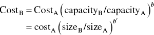
Table 7.11 Cost indices as annual averages.
Source: Adopted from indices published monthly by Chemical Engineering.
| Base year | Marshall‐Swift (1926 = 100) all industries | Chemical engineering plant cost index (1958 = 100) |
| 1984 | 780.4 | 322.7 |
| 1985 | 789.6 | 325.3 |
| 1986 | 797.6 | 318.4 |
| 1987 | 813.6 | 323.8 |
| 1988 | 852.0 | 342.5 |
| 1989 | 895.1 | 355.4 |
| 1990 | 915.1 | 357.6 |
| 1991 | 930.6 | 361.3 |
| 1992 | 943.1 | 358.2 |
| 1993 | 964.2 | 359.2 |
| 1994 | 993.4 | 328.1 |
| 1995 | 1027.5 | 381.1 |
| 1996 | 1039.1 | 381.7 |
| 1997 | 1056.8 | 386.5 |
| 1998 | 1061.9 | 389.5 |
| 1999 | 1068.3 | 390.6 |
| 2000 | 1080.6 | 392.6 |
| 2001 | 1093.9 | 394.3 |
| 2002 | 1104.2 | 395.6 |
| 2003 | 1123.6 | 402.0 |
| 2004 | 1178.5 | 444.2 |
| 2005 | 1244.5 | 468.2 |
| 2006 | 1302.3 | 499.6 |
| 2007 | 1373.3 | 525.4 |
| 2008 | 1449.3 | 575.4 |
| 2009 | 1486.6 | 521.9 |
| 2010 | — | 550.8 |
| 2011 | — | 585.7 |
where
- capacityB = equipment throughput, in standard units of cfm, gpm, etc.
- sizeB = equipment size, in standard units of 2 ft2, ft3, etc.
- b, b′ = constant
The exponents b and b′ vary from 0.5 to 0.8 and will average between 0.6 and 0.7 for many types of equipment. Typical exponent values for various types of air pollution control equipment are shown in Table 7.12.
7.13 Waste‐to‐Energy
Waste‐to‐energy (WtE) or energy‐from‐waste (EfW) is the process of generating energy in the form of electricity and/or heat from the primary treatment of waste. WtE is a form of energy recovery. Most WtE processes produce electricity and/or heat directly through combustion, or produce a combustible fuel commodity, such as methane, methanol, ethanol, or synthetic fuels.
Gasification and pyrolysis processes have been known and used for centuries and for coal as early as the eighteenth century. Development technologies for processing (residual solid mixed waste) has only become a focus of attention in recent years stimulated by the search for more efficient energy recovery (Fichtner Consulting Engineers 2004).
Municipal solid waste (MSW) to a large extent is of biological origin (biogenic), e.g. paper, cardboard, wood, cloth, food scraps. Typically, half of the energy content in MSW is from biogenic material. Consequently, this energy is often recognized as renewable energy according to the waste input.
7.13.1 Methods
7.13.1.1 Incineration
Incineration, the combustion of organic material such as waste with energy recovery, is the most common WtE implementation. All new WtE plants in OECD countries incinerating waste (residual MSW, commercial, industrial, or refuse‐derived fuel [RDF]) must meet strict emission standards, including those on nitrogen oxides (NOx), sulfur dioxide (SO2), heavy metals, and dioxins. Hence, modern incineration plants are vastly different from old types, some of which neither recovered energy nor materials. Modern incinerators reduce the volume of the original waste by 95–96%, depending upon composition and degree of recovery of materials such as metals from the ash for recycling.
Incinerators may emit fine particulate, heavy metals, trace dioxin, and acid gas, even though these emissions are relatively low from modern incinerators. Other concerns include proper management of residues: toxic fly ash, which must be handled in hazardous waste disposal installation as well as incinerator bottom ash, which must be reused properly.
Critics argue that incinerators destroy valuable resources and they may reduce incentives for recycling. The question, however, is an open one, as European countries which recycle the most (up to 70%) also incinerate to avoid landfilling.
Incinerators have electric efficiencies of 14–28%. In order to avoid losing the rest of the energy, it can be used for, e.g., district heating (cogeneration). The total efficiencies of cogeneration incinerators are typically higher than 80% (based on the lower heating value of the waste).
The method of incineration to convert MSW is a relatively old method of WtE production. Incineration generally entails burning waste (residual MSW, commercial, industrial, and RDF) to boil water which powers steam generators that make electric energy and heat to be used in homes, businesses, institutions, and industries. One problem associated is the potential for pollutants to enter the atmosphere with the flue gases from the boiler. These pollutants can be acidic and in the 1980s were reported to cause environmental damage by turning rain into acid rain. Since then, the industry has removed this problem by the use of lime scrubbers and ESPs on smokestacks. By passing the smoke through the basic lime scrubbers, any acids that might be in the smoke are neutralized which prevents the acid from reaching the atmosphere and hurting the environment. Many other devices, such as FFs, reactors, and catalysts destroy or capture other regulated pollutants. According to the New York Times, modern incineration plants are so clean that “many times more dioxin is now released from home fireplaces and backyard barbecues than from incineration.” According to the German Environmental Ministry, “because of stringent regulations, waste incineration plants are no longer significant in terms of emissions of dioxins, dust, and heavy metals.”
7.13.2 Other Technologies
There are a number of other new and emerging technologies that are able to produce energy from waste and other fuels without direct combustion. Many of these technologies have the potential to produce more electric power from the same amount of fuel than would be possible by direct combustion. This is mainly due to the separation of corrosive components (ash) from the converted fuel, thereby allowing higher combustion temperatures in, e.g., boilers, gas turbines, internal combustion engines, and fuel cells. Some are able to efficiently convert the energy into liquid or gaseous fuels.
Thermal technologies:
- Gasification: produces combustible gas, hydrogen, synthetic fuels
- Thermal depolymerization: produces synthetic crude oil, which can be further refined
- Pyrolysis: produces combustible tar/bio‐oil and chars
- Plasma arc gasification or plasma gasification process (PGP): produces rich syngas including hydrogen and carbon monoxide usable for fuel cells or generating electricity to drive the plasma arch, usable vitrified silicate and metal ingots, salt, and sulfur
Non‐thermal technologies:
- Anaerobic digestion: biogas rich in methane
- Fermentation production: examples are ethanol, lactic acid, hydrogen
- Mechanical biological treatment (MBT)
- MBT + anaerobic digestion
- MBT to refuse derived fuel
7.13.3 Global Developments
During the 2001–2007 period, the WtE capacity increased by about 4 million MT/Y. Japan and China each built several plants based on direct smelting or on fluidized bed combustion of solid waste. Japan is the largest user in thermal treatment of MSW in the world, with 40 million T. Some of the newest plants use stoker technology and others use the advanced oxygen enrichment technology. There are also over one hundred thermal treatment plants using relatively novel processes such as direct smelting, the Ebara fluidization process, and the thermoselect JFE gasification and melting technology process. In India its first energy bio‐science center was developed to reduce the country's greenhouse gases and its dependency on fossil fuel. As of June 2014, Indonesia had a total of 93.5 MW installed capacity of WtE, with a pipeline of projects in different preparation phases together amounting to another 373 MW of capacity.
Biofuel Energy Corporation of Denver, CO, opened two new biofuel plants in Wood River, Nebraska, and Fairmont, Minnesota, in July 2008. These plants use distillation to make ethanol for use in motor vehicles and other engines. Both plants are currently reported to be working at over 90% capacity. Fulcrum BioEnergy Incorporation located in Pleasanton, California, is building a WtE plant near Reno, Nevada. The plant is scheduled to open in 2020. https://fulcrum‐bioenergy.com/facilities. BioEnergy Incorporation predicts that the plant will produce approximately 10.5 MG/year of ethanol from nearly 200 000 T/Y of MSW.
WtE technology includes fermentation, which can take biomass and create ethanol, using waste cellulosic or organic material. In the fermentation process, the sugar in the waste is changed to carbon dioxide and alcohol, in the same general process that is used to make wine. Normally, fermentation occurs with no air present. Esterification can also be done using WtE technologies, and the result of this process is biodiesel. The cost effectiveness of esterification will depend on the feedstock being used, and all the other relevant factors such as transportation distance, amount of oil present in the feedstock, and others. Gasification and pyrolysis by now can reach gross thermal conversion efficiencies (fuel to gas) up to 75%; however, a complete combustion is superior in terms of fuel conversion efficiency. Some pyrolysis processes need an outside heat source which may be supplied by the gasification process, making the combined process self‐sustaining.
7.13.3.1 Carbon Dioxide Emissions
In thermal WtE technologies, nearly all of the carbon content in the waste is emitted as carbon dioxide (CO2) to the atmosphere (when including final combustion of the products from pyrolysis and gasification; except when producing bio‐char for fertilizer). MSW contain approximately the same mass fraction of carbon as CO2 itself (27%), so treatment of 1 MT (1.1 short tons) of MSW produce approximately 1 MT (1.1 short tons) of CO2.
In the event that the waste was landfilled, 1 MT (1.1 short tons) of MSW would produce approximately 62 m3 (2200 ft3) methane via the anaerobic decomposition of the biodegradable part of the waste. This amount of methane has more than twice the global warming potential than the 1 MT (1.1 short tons) of CO2, which would have been produced by combustion. In some countries, large amounts of landfill gas are collected, but still the global warming potential of the landfill gas emitted to atmosphere in, e.g., the United States in 1999 was approximately 32% higher than the amount of CO2 that would have been emitted by combustion.
In addition, nearly all biodegradable waste is biomass. That is, it has biological origin. This material has been formed by plants using atmospheric CO2 typically within the last growing season. If these plants are regrown, the CO2 emitted from their combustion will be taken out from the atmosphere once more.
Such considerations are the main reason why several countries administrate WtE of the biomass part of waste as renewable energy. The rest – mainly plastics and other oil and gas derived products – is generally treated as nonrenewables.
7.13.4 Examples of WtE Plants
According to ISWA there are 431 WtE plants in Europe (2005) and 89 in the United States (2004). The following are some examples of WtE plants.
Waste incineration WtE plants:
- Lee County Solid Waste Resource Recovery Facility, Fort Myers, Florida, USA (1994)
- Montgomery County Resource Recovery Facility in Dickerson, Maryland, USA (1995)
- Essex County Resource Recovery Facility, Newark, New Jersey, USA (1996)
- Spokane Waste‐to‐Energy Facility, Washington, USA (1996)
- Spittelau (1971), and Flötzersteig Vienna, (Wien Energie), Austria (1963)
- SYSAV Waste‐to‐Energy Plant, Malmö, Sweden (2003 and 2008)
- Stoke Incinerator, Stoke‐on‐Trent, England, UK (1989)
- Teesside EfW plant near Middlesbrough, North East, England, UK (1998)
- Edmonton Incinerator in Greater London, England, UK (1974)
- Burnaby Waste‐to‐Energy Facility, Metro Vancouver, Canada (1988)
- Timarpur‐Okhla Waste to Energy Plant, New Delhi, India (2001)
- Algonquin Power, Brampton, Ontario, Canada (1990)
7.13.5 Case Study: Energy Recovery from Municipal Solid Waste: Profitable Pollution Prevention at the City of Spokane, Washington (see Appendix G)
7.14 Sustainable Economy and the Earth
Evidence that the economy is in conflict with Earth's natural systems can be seen in the daily news reports of collapsing fisheries, shrinking forests, eroding soils, deteriorating rangelands, expanding deserts, rising carbon dioxide levels, falling water tables, rising temperatures, more destructive storms, melting glaciers, rising sea level, dying coral reefs, and disappearing species. These trends, which mark an increasingly stressed relationship between the economy and the Earth's ecosystem, are taking a growing economic toll. At some point, this could overwhelm the worldwide forces of progress, leading to economic decline. The challenge for our generation is to reverse these trends before environmental deterioration leads to long‐term economic decline, as it did for so many earlier civilizations.
7.14.1 What Is a Sustainable Economy?
An environmentally sustainable economy – an eco‐economy – requires that the principles of ecology be observed in establishing the framework for formulating economic policy and that economists understand that all economic activity, indeed all life, depends on the Earth's ecosystems – the complex of individual species living together, interacting with each other, and with their physical habitat. Millions of plant and animal species exist in an intricate balance, woven together along the food chain by nutrient cycles, the hydrological cycle, and global climate systems. Economists know how to translate goals into policy. Economists and ecologists, along with engineers, scientists, and policy makers, working together are being challenged to design and build an eco‐economy, one that can sustain progress (Brown 2001a, b; Western Governors' Association, 3 December 2004).
Through industrial ecology, eco‐industrial parks, eco‐efficiency, Zero Discharge manufacturing, and engineering new products from agricultural materials (biorenewable resources), an eco‐economy that facilitates sustainable economic progress offer the potential for the achievements, over the long‐term, of a sustainable economy and a healthy planet. Humankind has gone outside the biotic environment for the majority of its material needs only recently. Plant‐based resources were the predominant source of energy, organic chemicals, and fibers in the West as recently as 150 years ago, and they continue to play important roles in many developing countries.
The transition to nonbiological (or nonrenewable) sources of energy and materials was relatively swift and recent in the history of the world. Biorenewable resources are by definition sustainable natural resources; that is, they are self‐renewing at a rate that ensures their availability for use by future generations. Biorenewable resources can be converted into either bioenergy or biobased engineering products. Bioenergy, also known as biomass energy, is the result of the conversion of the chemical energy of a biorenewable resource into heat and stationary power. Biobased products include transportation fuels, chemicals, and natural fibers derived from biorenewable resources. Transportation fuels are generally liquid fuels, such as ethanol or biodiesel, but compressed hydrogen and methane have also been proposed and evaluated for use in vehicular propulsion.
Chemicals may include pharmaceuticals, nutraceuticals, and other fine chemicals, but the emphasis here is on commodity chemicals, which produce high demands for biorenewable resources. An example is polylactic acid, which is derived from the fermentation of sugars hydrolyzed from cornstarch and can be converted into biobased polymers used in a variety of consumer products such as carpets.
Figure 7.9 Example of supply curves to different kinds of biorenewable resources.
The cost of a biorenewable resource is related to the demand for the resource by a supply curve. Figure 7.9 is a generalized representation of a supply curve for the three kinds of biorenewable resources. The cost of biorenewable resources is highly variable and dependent on local conditions of supply and demand. This is particularly true for the costs involved in processing residue and wastes. Table 7.13 provides an estimate of the availability and cost of several kinds of residues and wastes along with a comparison of the costs of a few crop. The cultivation and harvesting of dedicated energy crops, on the other hand, is amenable to standardized cost estimating since information on “unit operation,” such as planting, fertilizing, and harvesting, can be readily obtained from knowledgeable sources (Brown 2001b).
7.14.2 Costs of Manufacturing Various Biobased Products and Energy
Over the next decades, a much larger fraction of fuels, chemicals, and materials will be produced from renewable plant materials. These biobased industrial products offer the potential for a much more sustainable economy based on environmentally superior products. This section briefly describes the associated costs of producing electricity, fuels, and chemicals from various feedstocks using biorenewable resources.
Table 7.13 Availability and cost of potential feedstocks.
Source: Crop data from Polman (1994) and Waste and residue data from Lynd (1996).
| Feedstocks | Production (106 T/Y) | Price (194 $/kg) |
| Corn | 191 | 0.09 |
| Potato | 17 | 0.16 |
| Sorgham | 16 | 0.09 |
| Beet molasses | 1 | 0.09 |
| Cane molasses | 1 | 0.03 |
| Sugar cane | 25 | 0.03 |
| Agricultural residues | ||
| Low cost | 4 | 12.9 |
| Mid cost | 36 | 38.8 |
| High cost | 50 | 47.4 |
| Forest residue‐logging | ||
| Low cost | 3 | 12.9 |
| Mid cost | 3 | 25.9 |
| High cost | 3 | 43.1 |
| Forest residue mill | 3 | 17.2 |
| Municipal solid waste | ||
| Mixed paper | 26 | 0–19 |
| Packaging | 14 | 0–5.2 |
| Urban wood | 3.5 | 12.9–25.9 |
| Yard waste | 11 | 0.12.9 |
7.14.2.1 Electricity from Combustion of Biomass
The capital and operating costs for steam power plants fired with biomass are relatively well known because of significant operating experience with these systems. The capital cost for a new plant ranges between $1400 and $1800/kW capacity. Accordingly, a 50‐MW biomass plant based on direct‐combustion would cost approximately $80 million. On the basis of a target price of $41.90/GJ for biomass, the cost of production for direct‐fired biomass power is about $0.06/kWh (Environmental Law & Policy Center 2001).
7.14.2.2 Electricity from Gasification of Biomass
The capital cost for a gasification plant, including fuel feeding and gas cleanup, is dependent on both the size and the operating pressure of the system. In the United States, an atmospheric‐pressure gasifier producing 50 MW thermal energy would cost about $15 million. A gasification/gas‐turbine power plant producing 50 MW of electricity would have total capital cost of between $75 and $138 million (between $1500 and $2750/kW), the smaller number reflecting improved technical know‐how after building at least ten plants. Electricity production costs would range from $0.05 to $0.09/kWh if fuel is available at an optimistic price range of $1.00–$1.50/GJ.
Capital costs for high‐temperature fuel cells suitable for integrated gasification/fuel cell power plants currently cost $3000/kW. Molten carbonate fuel cells are expected to be $1500/kW at the time of market entry, decreasing to about $1000/kW for a commercially mature unit. The cost of electricity from a mature unit operating on natural gas is projected to be between $0.049 and $0.085/kWh. More attractive economics result if less expensive fuel is available. The cost of electricity generated from landfill gas using mature fuel‐cell technology is expected to be comparable to that for an internal combustion engine/electric generator set, i.e., about $0.05/kWh (Bridgewater 1995; Hirschenhoofer et al. 1994; William and Larson 1993).
7.14.2.3 Biogas from Anaerobic Digestion
Anaerobic digestion is commercially developed for the purpose of treating wastewater. Power production from anaerobic digestion is in its infancy. The methane generated is often fired in internal combustion engines to produce electricity in an effort to help offset costs of waste treatment, but there are no immediate prospects for it to replace natural gas. Capital costs for anaerobic digestion facilities processing more than 200 T/day of volatile solids are estimated to be between $44 000 and $132 000 for each T/day of volatile solids processed. Methane yields will be approximately 0.38 m3/kg of volatile solids. Thus, a 200 T/day anaerobic digestion plant could produce 28 million m3 of methane per year, representing almost 2900 GJ/day of chemical energy. Projected operating costs for producing methane from dedicated energy crops were in the range of $5–6/GJ in 1986 dollars. In comparison, the cost of natural gas in the United States, which shows large seasonal and geographical variations, ranges between $1.90 and $4/GJ. In niche markets, where the feedstock is inexpensive and natural gas is not available, biogas can be a viable alternative energy source (Benson et al. 1986). A similar biogas manufacturing using poultry WtE by catalytic steam gasification process is described in Chapter 10.
7.14.2.4 Ethanol from Biomass
The cost of producing ethanol from biomass varies tremendously depending on the feedstock employed, the size and management of the facility and the market value of coproducts generated as part of some conversion processes. Cost information for ethanol plants to be built in the United States is most reliable for those using cornstarch, the basis of the US ethanol industry. A 5000 barrel/day plant (about 265 million l/day) built from the ground up will have a capital cost of about $140 million in 1987 dollars, or $0.53/l of annual capacity. Smaller facilities can have capital costs as high as $0.79/l of annual capacity, and poorly designed facilities of any size may cost $1.06/l of annual capacity. On the other hand, ethanol plants that are built from existing facilities, such as refineries or chemical plants, or ethanol plants integrated into a larger industrial facility, can have substantially lower capital costs, often in the range of $0.26–0.40/l of annual capacity.
Low‐end production costs are about $0.26/l. However, the volumetric heating value of ethanol is only 66% that of gasoline. This production cost, therefore, is equivalent to gasoline selling for $0.39/l before tax, transportation, or profit. In contrast, refinery price for gasoline in 1990 dollars was $0.20/l. Currently, the economics of fermentation are such the commercial viability of ethanol is entirely dependent on government incentives in the form of tax credit, currently $0.16 for each liter of ethanol used for fuel blending. Also, a strong market for fermentation by‐products is key factor in the economic viability of ethanol‐from‐corn.
Technology to convert lignocellulose to sugar is expected to reduce the cost of fuel ethanol, although dedicated economic information is not currently available. Capital cost for a 5000 barrel/day plant to produce ethanol from lignocellulose using simultaneous saccharification and fermentation is estimated to be $175 million (1994 dollars). Assuming wood costs $42/dry ton, ethanol can be produced for about $0.31/l. Combining economies of scale with advances in processing technology are projected to decrease production costs to 40.31/l. However, some reports have suggested that ethanol from cellulose will have to cost as little as $0.08–0.11/l to be competitive with the gasoline prices anticipated early in the twenty‐first century (Lynd et al. 1996; National Advisory Panel 1987).
7.14.2.5 Methanol from Biomass‐Derived Syngas
Capital investment for a 7500 barrel/day plant to produce methanol from biomass would be about $280 million in 1991 dollars. The cost of methanol from $40/dry ton of wood is projected to be about $0.27/l. Since the volumetric heating value of methanol is only 49% that of gasoline, the production cost from this plant is equivalent to gasoline selling for $0.55/l. Methanol from natural gas can be produced at significantly lower cost, but this assumes much larger plant capacities to capture economies of scale. Such large plants are not feasible for widely dispersed biomass feedstocks. New methanol‐synthesis technologies may be able to significantly reduce this price. The U.S. Department of Energy's methanol from biomass program has a goal of $0.15/l ($7.90/GJ) based on feedstock cost of $1.90/GJ (Klass 1998).
7.14.2.6 Bio‐Oil from Fast Pyrolysis
Capital investment for a 5000 barrel/day plant to produce pyrolysis liquids would be $63 million in 1987 dollars. Assuming biomass feedstock was available at $1.70/GJ, this size plant could produce pyrolysis liquids for $0.18/l, which has an energy value of $6.70/GJ (Elliott et al. 1990).
7.14.2.7 Biodiesel from Vegetable Oils
Capital costs for a biodiesel facility are relatively modest, costing about $250 000 for a 50 barrel/day (3.2 million l/year). However, feedstock costs for production of biodiesel are relatively higher than feedstocks for production of other kinds of fuel, ranging from $0.16 to $0.26/l for waste fats to $0.53–0.79/l for vegetable oils. Under the best scenarios, a biodiesel plant might produce fuel for $0.44/l. Diesel fuel produced from petroleum typically sells for less than $0.25/l (Gavett et al. 1993).
7.14.2.8 Succinic Acid
Succinic acid is used in producing food and pharmaceutical products, surfactants and detergents, biodegradable solvents and plastics, and ingredients to stimulate animal and plant growth. Although it is a common metabolite formed by plants, animals, and microorganisms, its current commercial production of 15 000 T/Y is from petroleum. However, the recently discovered rumen organism Actinobacillus succinogenes produces succinic acid with yields as high as 110 g/l, offering prospects for producing this chemical from biorenewable resources. In contrast to most other commercial fermentations, the process consumes CO2 and, integrated with a process like ethanol fermentation, succinic acid production could contribute to reduction in greenhouse gas emissions.
Optimum yields occur under pH conditions where succinate salt rather than free acid is produced. Thus, recovery entails concentration of the salt, conversion back to free acid, and polishing of the acid to the desired purity. Downstream purification can account for 60–70% of the product cost.
7.14.2.9 Lactic Acid
Lactic acid, a three‐carbon molecule, is used in the production of polylactide resin, a biodegradable polymer expected to compete with polyethelene and polystyrene in the synthetic fibers and plastic markets. Lactic acid is currently produced by milling corn, separating the starch, hydrolyzing the starch to glucose, and anaerobically fermenting the glucose to lactic acid with Bacillus dextrolactius or Lactobacillus delbrueckii. Esterification with ethanol produces ethyl lactate, which can be polymerized to polylactate resin.
Problems
- 7.1 A manufacturing process has present operating costs of $10.9 million annually and waste disposal costs of 3.3 million. The plant manager wishes to upgrade the process by installing new equipment at a capital cost of $23.3 million. This will reduce the annual operating and waste disposal costs to $7.1 and $1.4 million respectively. Compare the two processes on a present worth basis, assuming no salvage value. Use 12% interest for 10 years as a basis for calculation.
- 7.2 (a) Should a project with
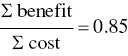 be undertaken? Explain your answer; (b) What are the drawbacks of relying on the benefit/cost ratio for justifying a project?
 - 7.3 A community plans to build a landfill to dispose of wastes for next 20 years. The cost estimates and expected revenue are as follows:
Landfill construction cost $7 600 000 Start‐up costs $500 000 Operation and maintenance costs per year $1 000 000 Tipping fees received per year $4 500 000 Assume that citizens will only support the new landfill facility if the benefit/cost ratio is greater than 1.5. At a 7% interest rate over the 20 years life, determine if the landfill should be built.
- 7.4 A county wants to build a toll‐free bridge over a river in order to take time off of a route that goes through the mountains. Benefits are decreased travel time, fewer accidents, reduced gas usage, less pollution, etc. Should be bridge be built? Benefit and cost data are given below.
Millions ($) Initial cost 40 Annual maintenance 12 Annual user benefits 49 Residual value 0 - 7.5 Given that a wet scrubber had a TIC of $800 000 in 2001, estimate the 2008 TIC using the two cost indices (Marshall‐Swift & Chemical Engineering Plant) presented in Table 7.11. Use a reasonable method to estimate the TIC in the year 2013.
- 7.6 A company uses a 50% solution of NaOH to maintain the pH of water circulated in one of its furnace exhaust scrubbers. The cost of the solution is $200/T free‐on‐board. The supplier says it would prefer to sell the company a 65% NaOH solution and the company says the water content is immaterial as long as the equivalent costs are the same including freight. If the freight is $15/T, what is the maximum price per ton the company should pay for the 65% solution?
- 7.7 An engineer has compiled the data below for two different project options – one that includes a comprehensive pollution prevention program/option and one that does not (data are given in a table below). From an economic point of view, which project should the engineer select? The lifetime of the equipment is 10 years and the interest rate is 10%.
Pollution prevention cost data:
Project with pollution prevention (W) ($) Project without pollution prevention (WO) ($) Equipment cost 1 294 000 1 081 000 Installation cost 786 000 659 000 Operating labor (per year) 39 900 8 500 Maintenance (per year) 43 000 17 000 Utilities (per year) 958 000 821 000 Overhead (per year) 51 300 13 900 Taxes, insurance and administr. (per year) 86 200 72 600 Credits (per year) 380 000 0 - 7.8 A small rural community with a population of 850 people generates recyclable solid waste, at an average rate of 2.0 lb/day/capita. The chemical composition of the wastes is C89.10H138.61O51.98N1. The approximate Btu values for individual materials in RDF can be calculated using the following equation:
where C, H, O, S, and N values are in wt%.
Determine
- the percentage distribution by weight of elements in the waste, round off the coefficients and set up a table
- the daily energy content of the waste that is received by a local WtE facility.
- 7.9 In the City of Aberdeen, Scotland, a landfill with a gas collection system is in operation and serves a population of 250 000. At a rate of (4.4 lb)/(person‐day) RDF from the city's solid waste is generated. Gas is produced at an annual rate of 2.8 l/lb at the city's landfill. The gas contains 60% methane. The gas recovery is about 20% of that generated. The heat content of the landfill gas is approximately 480 Btu/ft3 (this value is lower than the theoretical value because of dilution of methane with air during gas recovery). The landfill operator and the city have proposed to supply the methane to homes that would be built in the vicinity of the landfill. The homes are estimated to use an average of 95 × 106 Btu/year for heating and cooking. Peak usage during winter is 1.3 times the average usage. How many homes could be served by the energy generated at the landfill?
- 7.10 Recently, a cast iron leaf pressure filter with 100 ft2 was purchased for clarifying an inorganic liquid stream for $15 000. In a similar application, the company will need a 450 ft2 cast iron leaf pressure filter. The size exponent for this filter is 0.6. Estimate the purchased price of the 450 ft2 unit.
- 7.11 A stainless steel centrifuge costs $83 000 in 1990. What is the cost of that same centrifuge in 2001? Use the CE Index.
- 7.12 The delivered equipment cost (DEC) for a fixed‐bed carbon adsorption system with a capacity of 5000 acfm was $100 000 in 1994. Estimate the total installation cost of a similar system with a capacity of 7500 acfm in 2000. Assuming the size exponent for a carbon‐adsorption system is 0.7 and TIC is 1.5 times the DEC.
- 7.13 Search the literature on mercury emissions from coal‐fired power plants and make a brief report. In your report, address the following: total mercury emissions in the United States, range of mercury content in coal, US regulations dealing with mercury from coal‐fired power plants, and methods for controlling mercury (with approximate control efficiencies) in power plant exhaust gases.
- 7.14 A water resources project has produced benefits that equal $40 000 at the end of 20 years. Determine the PV of these benefits using a 6% interest rate? Determine the PV of the benefits at the end of the 20th year.
- 7.15 A water resources project has produced benefits that equal $20 000 at the end of the first year and increase on a uniform gradient series to $100 000 at the end of the 5th year. The benefits remain constant at $100 000 each year until the end of the year 25. Determine the PV of these benefits using a 6% interest rate?
- 7.16 Exhaust gas from a gas turbine facility (2 × 10⁵ lb/h steam capacity) flows at a rate of 100 000 dscfm at 1200 °F with a PM loading of 1.5 gr/dscfm. As part of PSD/Title V permitting process, a top‐down BACT analysis is needed in which the TAC and cost per ton of PM removal ($/T) to be evaluated for four control options: (i) MC, (ii) VS, (iii) ESPs, and (iv) FF. Calculate the $/T of PM removal by four control technologies using the TACs for four control options presented in Figure 7.7. Assume MC and VS have 90% and ESP and FF have 99.5% removal efficiencies, respectively.
References
- Air Pollution Training Institute (APTI) (1995). APTI Course 427 Lecture Note on Control of Gaseous Emissions. Research Triangle Park, NC: USEPA.
- Allen, D.T. and Rosselot, K.S. (1997). Pollution Prevention for Chemical Processes, 19–32. New York, NY, Chapter 2: Wiley.
- Benson, P.H., Hayes, T.D., and Isaacson, R. (1986). Regional and community approaches to methane from biomass and waste: an industry perspective. Proceedings Energy from Biomass and Waste X, Orlando, FL (April 1986).
- Bridgewater, A.V. (1995). The technical and economic feasibility of biomass gasification for power generation. Fuel 74: 631–653.
- Brown, L.R. (2001a). Eco‐Economy: Building an Economy for the Earth. New York, NY: W. W. Norton.
- Brown, R.C. (2001b). Biorenewable Resources: Engineering New Products from Agriculture. Iowa State Press.
- Burckle, J.O. and Ferguson, T.D. (2005). Advances in pollution prevention in the metal finishing industry. In: Toward Zero Discharge: Innovative Methodology and Technologies for Process Pollution Prevention (ed. T.K. Das). Hoboken, NJ: Wiley.
- Burgess, T.L., Gibson, A.G., Furstein, S.J., and Wachs, I.E. (2002). Converting waste gases from pulp mills into value‐added chemicals. Environmental Progress 21 (3): 137–141.
- California Air Resource Board (2000). Statewide Best Available Control Technology (BACT) Clearinghouse. South Coast Air Quality Management District (August 17). http://www.arb.ca.gov/bact/bact.htm (accessed 11 January 2019).
- Cluster Rule Regulation (1998). 40CFR Part 63, Subpart S (foul condensates), Section 63:446.
- Dalan, J. (2005). Brine concentrators for recycling wastewater. In: Toward Zero Discharge: Innovative Methodology and Technologies for Process Pollution Prevention (ed. T.K. Das). Hoboken, NJ: Wiley.
- Dalan, J. and Rosain, R. (1992). Zero Discharge Wastewater Treatment Facility for a 900 MW GCC Power Plant, Report No. EPRI TR‐100375. Palo Alto, CA: Electric Power Research Institute.
- Das, T.K. (1997). A pollution prevention strategy in the kraft pulp and paper manufacturing process technologies. Paper 188c, American Institute of Chemical Engineers National Meeting, Los Angeles, CA.
- Das, T.K. (1999a). Process pollution prevention advances in the pulp and paper industry. Paper 274b, American Institute of Chemical Engineers National Meeting, Dallas, TX.
- Das, T.K. (1999b). Process technology advances in the pulp and paper industry. Paper 273e, American Institute of Chemical Engineers National Meeting, Dallas, TX.
- Das, T.K. (2001). Qualitative Analysis of Control Technologies, Costs, and Environmental Impacts Analyses‐Wood‐fired Boiler RACT Determination. Air Quality Program, Washington Department of Ecology, Draft Report.
- Das, T.K. (2003). Hog‐Fuel Boiler's Reasonably Available Control Technology (RACT) Determination. Air Quality Program, Washington Department of Ecology, Olympia, Washington, Report #03‐02‐009, 137 pages. http://www.ecy.wa.gov/biblio/0302009.html (accessed 14 February 2019).
- Das, T.K. (2005). Toward Zero Discharge: Innovative Methodology and Technologies for Process Pollution Prevention. Hoboken, NJ: Wiley‐InterScience.
- Das, T.K. and Houtman, C. (2004). Evaluating chemical‐, mechanical‐, and bio‐pulping processes and its sustainability characterization using life cycle assessment. Environmental Progress Special Issue on Sustainability 23 (4): 347–357.
- Das, T.K. and Jain, A.K. (2001). Pollution prevention advances in pulp and paper processing. Environmental Progress 22 (2): 87–92.
- DaSilva, A. and Goodman, A. (2014). Reduce water consumption through recycling. Chemical Engineering Progress 110: 29–37.
- Dzombak, D.A. (2013). Use of treated municipal wastewater as power plant cooling system makeup water: tertiary treatment versus expanded chemical regimen for recirculating water quality management. Environmental Engineers and Scientists 49 (2): 30.
- Elliott, D.C., Osman, A., Borje Gevett, S. et al. (1990). Biomass for renewable energy and fuels. In: Energy from Biomass and Wastes XIII (ed. D.L. Klass). Chicago, IL: Institute of Gas Technology.
- Environmental Law and Policy Center (2001). Repowering the Midwest: the clean energy development plan for the Heartland. www.repowermidwest.org (accessed 18 February 2019).
- Ferguson, D., Hindin, B., Chen, A., and Monzyk, B. (2001). Picklex as a non‐polluting metal surface finishing pretreatment and pretreatment/conversion coating. Clean Products and Processes 2: 220–227.
- Ferguson, D. and Monzyk, B. (2003). Non‐polluting metal surface finishing pretreatment and pretreatment/conversion coating. Plating and Surface Finishing 90: 66–75.
- Ferguson, D. and Wilmoth, R. (2000). Cost‐effective control of hexavalent chromium air emissions from functional chromium electroplating. Environmental Health and Safety Solutions 1 (3): 10–19.
- Fichtner Consulting Engineers Ltd. (2004). The Viability of Advanced Thermal Treatment of MSW in the UK. London: ESTET.
- Fosberg, T. (1992). Case study: water recovery systems at the world's first zero effluent pulp mill. Proceedings of the International Water Conference‐51st Annual Meeting, Pittsburgh, USA (19–21 October 1992).
- Gavett, E.E., van Dyne, D., and Blasé, M. (1993). Fuel cells for distributed generation. In: Energy from Biomass and Waste XIII (ed. D.L. Klass). Chicago, IL: Institute of Gas Technology.
- Haussman, C. and Rosain, R. (1996). Power Plant Wastewater Treatment Technology Review Report, Report No. EPRI TR‐10781. Palo Alto, CA: Electric Power Research Institute.
- Heller, M., Shields, P.D., and Beloff, B. (1995). Environmental accounting case study: Amoco Yorktown refinery. In: Green Ledgers: Case Studies in Corporate Environmental Accounting (eds. D. Ditz, J. Ranganathan and D. Banks). Washington, DC: World Resources.
- Hirschenhoofer, J. H., Stauffer, D. B., and Engleman, R. R. (1994). Fuel Cells: A Handbook, Department of Energy Technical Report DOE/METC‐94/1006 (DE94004072). Washington, DC: United States Department of Energy. https://www.annualreviews.org/doi/abs/10.1146/annurev.energy.21.1.403 (accessed 24 September 2019).
- Kirk, R.E. and Othmer, D.F. (2004). Encyclopedia of Chemical Technology, 5e. Hoboken, NJ: Wiley.
- Klass, D.L. (ed.) (1998). Thermal conversion. In: Biomass for Renewable Energy, Fuels, and Chemicals. San Diego: Academic Press.
- Klinker, R. (1996). Successful implementation of a Zero Discharge program. TAPPI Journal 79 (1): 97–102.
- Lynd, L.R. (1996). Overview and evaluation of fuel ethanol from cellulosic biomass: technology, economics, the environment, and policy. Annual Review of Energy and the Environment 21: 403–465.
- Lynd, L.R., Elander, R.T., and Wyman, C.E. (1996). Likely features and costs of manure biomass ethanol technology. Applied Biochemistry and Biotechnology 57/58: 741–761.
- National Advisory Panel on Cost Effectiveness of Fuel Ethanol Production (1987). Fuel Ethanol Cost‐Effectiveness Study Final Report.
- National Council of the Paper Industry for Air and Stream Improvement, Inc. (NCASI) (1991). Progress in Reducing Water Use and Wastewater Loads in the U.S. Paper Industry, Technical Bulletin No. 603. Research Triangle Park, NC: NCASI.
- Paik, S.C. and Chung, J.S. (1996). Selective hydrogenation of sulfur dioxide with hydrogen to elemental sulfur over transition metal sulfide supported on AL2O3. Applied Catalysis B: Environment 8: 267–279.
- Perry, R.H. and Green, D.W. (1997). Perry's Chemical Engineers' Handbook, 7e, 9–10. New York, NY: McGraw‐Hill and 9–16.
- Peters, M.S. and Timmerhaus, K. (2002). Plant Design and Economics for Chemical Engineers, 5e. New York: McGraw‐Hill.
- Peters, M.S., Timmerhaus, K., and West, R.E. (2002). Plant Design and Economics for Chemical Engineers, 5e. New York, NY: McGraw‐Hill.
- Pinkerton, J.E. (1999). Trends in U.S. kraft mill TRS emissions. Tappi Journal 82 (4): 166–169.
- Pollution Prevention 1997: A National Progress Report. http://www.epa.gov/opptintr/p297/foreword.pdf (accessed 4 March 2019).
- Polman, K. (1994). Review and analysis of renewable feedstocks for the production of commodity chemicals. Applied Biochemistry and Biotechnology 45 (/46): 709–722.
- Shields, P., Heller, M., Kite, D., and Bellof, B. (1995). Environmental accounting case study: DuPont. In: Green Ledgers: Case Studies in Corporate Environmental Accounting (eds. D. Ditz, J. Ranganathan and D. Banks). Washington, DC: World Resources.
- Smook, G.A. (1992). Handbook for Pulp and Paper Technologies, 2e. Bellingham, WA: Angus Wilde Publications.
- Stander, L. and Theodore, L. (2008). Environmental Regulatory Calculations Handbook. Hoboken, NJ: Wiley.
- State of California (2001). South Coast Air Quality Management District Rule 1151 (amended December 1998) and Rule 1132 (adopted January 2001).
- Title 40 Code of Federal Regulation (CFR) (2019). Part 51, Subpart 1, Review of New Sources and Modifications.
- United State Congress (1990). Pollution Prevention Act of 1990. http://www.epa.gov/opptintr/p2home/p2policy/act1990.htm ().
- United State Congress (1994). Office of Technology Assessment.
- USEPA (1982). Control and Treatment Technologies for the Metal Finishing Industry: In‐Plant Changes, EPA 625/ 8‐82‐008. USEPA, Office of Research and Development.
- USEPA (1985). Environmental Regulations and Technology: The Electroplating Industry, EPA 625/ 10‐85‐001. USEPA, Office of Research and Development.
- USEPA (1992a). Facility Pollution Prevention Guide, EPA/600/R‐92/088. Washington, DC: Office of Research and Development.
- USEPA (1992b). Model Pollution Prevention Plan for the Kraft Segment of the Pulp and Paper industry, EPA/910/9‐92‐030. Seattle, WA: EPA Region 10.
- USEPA (1995a). Toxic Release Inventory (TRI) release data for fabricated metals facilities SIC 340. http://www.epa.gov/triexplorer (accessed 7 March 2019).
- USEPA (1995b). 40CFR261 Identification and Listing of Hazardous Wastes. Code of Federal Regulations, US GPO. http://www.gpoaccess.gov/cfr/index.html (accessed 19 March 2019).
- USEPA (1995c). An Introduction to Environmental Accounting as a Business Management Tool: Key Concepts and Terms, EPA 742‐R‐95‐001. London: ACCA.
- USEPA (1996). Office of Air Quality Planning and Standards (OAQPS), Control Cost Manual, EPA 453/B‐96‐001, 5e. Research Triangle Park, NC: USEPA, Office of Air Quality Planning and Standards.
- USEPA (1998). Metal finishing/electroplating industry: case studies. http://es.epa.gov/cooperative/topics/metcasestudies.html (accessed 20 March 2019).
- USEPA (2000). Approaching Zero Discharge in Surface Finishing, EPA/625/R‐99/008. Research Triangle Park, NC: USEPA, Office of Research and Development.
- USEPA (2001). Living the Vision: Accomplishments of the National Metal Finishing Strategic Goals Program, Research Triangle Park, NC. USEPA, Office of Research and Development. EPA 240‐R‐00‐007. www.strategicgoals.org (accessed 20 March 2019).
- USEPA (2003a). Environmental management systems: systematically improving your performance. MetFin_BizCase_15. http://www.epa.gov/ispd/metalfinishing/metfin_pdf/metfin_bizcase.pdf (accessed 22 March 2019).
- USEPA (2004). A Guide to Developing an Environmental Management System for Metal Finishing Facilities. Washington, DC: USEPA, Sector Strategies. http://www.epa.gov/sectors/metalfinishing/metfin_ems.html (accessed 27 March 2019)
- USEPA (2011). Clean Air Act, Section 812 Analyses on the Benefits and Costs of the Clean Air Act from 1990 to 2020. www.epa.gov/ora/sec812 (accessed 27 March 2019).
- Vatavuk, W.M. (2002). Control Cost Manual, Emissions Standards Division of the Office of Air Quality, Planning and Standards, EPA/452/B‐02‐001. USEPA.
- Wachs, I.E. (1999a). Treating methanol‐containing waste gas streams. US Patent 5,907,066.
- Wachs, I.E. (1999b). Production of formaldehyde from methyl mercaptans. US Patent 5,969,191.
- Western Governors' Association (2004). Principles for environmental management in the west (3 December 2003). http://www.westgov.org/wga/policy (accessed 22 February 2004).
- William, R.H. and Larson, E.D. (1993). Fossil energy. In: Advances in Gasification‐Based Biomass Generation, Renewable Energy: Source for Fuels and Electricity (eds. T.B. Johnson, H. Kelly, A.K. Reddy and R.H. Williams). Washington, DC: Island Press.
Notes
- 1 Much of this material was derived from the Section 9.2.3 Burckle and Ferguson (2005).
- 2 MT/Y = metric tons per year.