3
Industrial Pollution Sources, Its Characterization, Estimation, and Treatment
3.1 Introduction
This chapter provides a summary of industrial wastewater sources, wastewater characteristics, wastewater treatment, reuse and discharge, industrial sources of air pollutions, inventories, air pollution control, solid waste and hazardous waste characteristics, treatments, and management.
Industrial waste is the waste produced by industrial activity which includes any material that is rendered useless during a manufacturing process such as that of factories, industries, mills, and mining operations. It has existed since the start of the Industrial Revolution (Pink 2006). Some examples of industrial wastes are chemical solvents, paints, sandpaper, paper products, industrial by‐products, metals, plastics, and radioactive wastes.
Toxic waste, chemical waste, industrial solid waste, and municipal solid waste are designations of industrial wastes. Sewage treatment plants can treat some industrial wastes, i.e. those consisting of conventional pollutants such as biochemical oxygen demand (BOD), chemical oxygen demand (COD), suspended solid (SS), and total suspended solid (TSS). Industrial wastes containing toxic pollutants require specialized treatment systems (United States Code, Clean Water Act, Section 402(p) 33 U.S. Code §1342(p) 1999).
3.2 Wastewater Sources
3.2.1 Point Source
Point source water pollution refers to contaminants that enter a waterway from a single, identifiable source, such as a pipe or ditch. Examples of sources in this category include discharges from a factory, a sewage treatment plant or a publicly owned treatment works (POTWs), or a city storm drain. The US Clean Water Act (CWA) defines point source for regulatory enforcement purposes (United States Code Clean Water Act Section 502 (14) 33 U.S.S 1362(14) 1999). The CWA definition of point source was amended in 1987 to include municipal storm sewer systems, as well as industrial storm water, such as from construction sites.
3.2.2 Nonpoint Source
Nonpoint source (NPS) pollution refers to diffuse contamination that does not originate from a single discrete source. NPS pollution is often the cumulative effect of small amounts of contaminants gathered from a large area. A common example is the leaching out of nitrogen compounds from fertilized agricultural lands (Moss 2008). Nutrient runoff in storm water from “sheet flow” over an agricultural field or a forest is also cited as examples of NPS pollution.
Contaminated storm water washed off of parking lots, roads and highways, called urban runoff, is sometimes included under the category of NPS pollution. However, because this runoff is typically channeled into storm drain systems and discharged through pipes to local surface waters, it becomes a point source.
Fugitive emissions are also NPS pollution in that the emissions of gases or vapors take place from pressurized equipment due to leaks and other unintended or irregular releases of gases, mostly from industrial activities. As well as the economic cost of lost commodities, fugitive emissions contribute to air pollution and climate change.
3.3 Wastewater Characteristics
Prior to about 1940, most municipal wastewater was generated from domestic sources. After 1940, as industrial development in the United States grew significantly, increasing amounts of industrial wastewater have been and continue to be discharged into municipal collection systems. The amounts of heavy metals and synthesized organic compounds generated by industrial activities have increased; some 10 000 new organic compounds are added each year. Many of these compounds are now found in the wastewaters.
As technological changes take place in manufacturing, changes also occur in the compounds discharged and the resulting wastewater characteristics. Numerous compounds generated from industrial processes are difficult and costly to treat by conventional wastewater treatment processes. Therefore, effective industrial pretreatment becomes an essential part of an overall water quality management program. Enforcement of an industrial pretreatment program is a daunting task; some of the regulated pollutants still escape to the municipal wastewater collection system and must be treated. In the future with the objective of pollution prevention, every effort should be made by industrial discharges to assess the environmental impacts of any new compounds that may enter the wastewater stream before being approved for use. If a compound cannot be treated effectively with existing technology, it should not be used.
The wastewater from industries varies greatly in both flow and concentration of pollutants. So, it is impossible to assign fixed values to their constituents. In general, industrial wastewaters may contain suspended, colloidal, and dissolved (mineral and organic) solids. In addition, they may be either excessively acidic or alkaline and may contain high or low concentrations of colored matter. These wastes may contain inert, organic, or toxic materials and possibly pathogenic bacteria. These wastes may be discharged into the sewer system provided they have no adverse effect on treatment efficiency or undesirable effects on the sewer system. It may be necessary to pretreat (Section 3.5.2) the wastes prior to release to the municipal system or it is necessary to make a full treatment when the wastes will be discharged directly to surface or ground waters.
The physical and chemical characterization presented below is valid for most wastewaters, both industrial and municipal.
3.3.1 Physical Characteristics
The principal physical characteristics of wastewater include solids content, color, odor, and temperature.
3.3.2 Total Suspended Solids
The total solids in a wastewater consist of the insoluble or total suspended solids and the soluble compounds dissolved in water. The suspended solids content is found by drying and weighing the residue removed by the filtering of the sample. When this residue is ignited the volatile solids are burned off. Volatile solids are presumed to be organic matter, although some organic matter will not burn and some inorganic salts break down at high temperatures. The organic matter consists mainly of proteins, carbohydrates and fats. Between 40 and 65% of the solids in an average wastewater are suspended. Settleable solids, expressed as milligrams per liter (mg/l), are those that are removed by sedimentation. Usually about 60% of the suspended solids in a wastewater are settleable (Crites and Tchbanoglous 1998). Solids may be classified in another way as well: those that are volatilized at a high temperature (600 °C) and those that are not. The former are known as volatile solids, the latter as fixed solids. Usually, volatile solids are organic.
3.3.3 Color
Color is a qualitative characteristic that can be used to assess the general condition of wastewater. Wastewater that is light brown in color is less than six hours old, while a light‐to‐medium grey color is characteristic of wastewaters that have undergone some degree of decomposition or that have been in the collection system for some time. Lastly, if the color is dark grey or black, the wastewater is typically septic, having undergone extensive bacterial decomposition under anaerobic conditions. The blackening of wastewater is often due to the formation of various sulphides, particularly ferrous sulphide. This results when hydrogen sulphide produced under anaerobic conditions combines with divalent metal, such as iron, which may be present. Color is measured by comparison with standards.
3.3.4 Odor
The determination of odor has become increasingly important, as the general public has become more concerned with the proper operation of wastewater treatment facilities. The odor of fresh wastewater is usually not offensive, but a variety of odorous compounds are released when wastewater is decomposed biologically under anaerobic conditions. The different unpleasant odors produced by certain industrial wastewater are presented in Table 3.1.
3.3.5 Temperature
The temperature of wastewater is commonly higher than that of the water supply because warm municipal water has been added. The measurement of temperature is important because most wastewater‐treatment schemes include biological processes that are temperature dependent. The temperature of wastewater will vary from season to season and also with geographic location. In cold regions, the temperature will vary from about 7 to 18 °C, while in warmer regions the temperatures vary from 13 to 24 °C (Crites and Tchobanoglous 1998).
Table 3.1 Unpleasant odors in some industries.
Source: From Eckenfelder (2000).
| Industries | Origin of odors |
| Cement works, Lime Kilns | Dibutyl amines, mercaptans, dibutylsulfide, hydrogen sulfide, sulfur dioxide |
| Food industries | Acetic acid, acetaldehyde |
| Food industries (fish) | Butyl amine, mercaptans, dimethyl sulfide, amines |
| Pharmaceutical industries | Fermentation by‐product produces |
| Pulp and paper industries (kraft) | Total reduced sulfur compounds, TRS: (hydrogen sulfide, mercaptans, methyl disulfide, dimethyl disulfide), sulfur dioxide |
| Rubber industries | Sulfides, mercaptans |
| Textile industriesa | Phenyl mercaptan, phenolic compounds |
| Tomato cannery | Acetic acid, acetaldehyde, thiophenol |
3.4 Chemical Characteristics
3.4.1 Inorganic Chemicals
The principal chemical tests include free ammonia, inorganic nitrogen as nitrate, nitrite, organic phosphorus, and inorganic phosphorus. Nitrogen and phosphorus are important because these two nutrients are responsible for the growth of aquatic plants. Other tests such as chloride, sulphate, pH, and alkalinity are performed to assess the suitability of reusing treated wastewater and in controlling the various treatment processes (Rouessac and Rouessac 2007).
Trace elements, which include some heavy metals, are not determined routinely, but trace elements may be a factor in the biological treatment of wastewater. All living organisms require varying amounts of some trace elements such as iron, copper, zinc, and cobalt for proper growth. Heavy metals can also produce toxic effects; therefore, determination of the amounts of heavy metals is especially important where the further use of treated effluent or sludge is to be evaluated. Many metals are also classified as priority pollutants such as arsenic, cadmium, chromium, mercury, etc.
Measurements of gases such as hydrogen sulphide, oxygen, methane, and carbon dioxide are made to help the system to operate. The presence of hydrogen sulphide needs to be determined not only because it is an odorous and very toxic gas but also because it can affect the maintenance of long sewers on flat slopes, since it can cause corrosion. Measurements of dissolved oxygen are made in order to monitor and control aerobic biological treatment processes. Methane and carbon dioxide measurements are used in connection with the operation of anaerobic digesters.
3.4.2 Organic Chemicals
Over the years, a number of different tests have been developed to determine the organic content of wastewaters. In general, the tests may be divided into those used to measure gross concentrations of organic matter greater than about 1 mg/l and those used to measure trace concentrations in the range of 10−12–10−3 mg/l. Laboratory methods commonly used today to measure gross amounts of organic matter (>1 mg/l) in wastewater include (i) BOD, (ii) COD, and (iii) total organic carbon (TOC). Trace organics in the range of 10−12–10−3 mg/l are determined using instrumental methods including gas mass spectroscopy and chromatography. Specific organic compounds are determined to assess the presence of priority pollutants (Metcalf & Eddy 2003). The BOD, COD, and TOC tests are gross measures of organic content and as such do not reflect the response of the wastewater to various types of biological treatment technologies.
3.4.3 Volatile Organic Compounds
Volatile organic compounds (VOCs), such as benzene, toluene, xylenes, trichloroethane, dichloromethane, and trichloroethylene (TCE), are common soil pollutants in industrialized and commercialized areas. One of the more common sources of these contaminants is leaking underground storage tanks. Improperly discarded solvents and landfills, built before the introduction of current stringent regulations, are also significant sources of soil VOCs. Many of organic substances are classified as priority pollutants such as PCBs, polycyclic aromatic, acetaldehyde, formaldehyde, 1,3‐butadiene, 1,2‐dichloroethane, dichloromethane, hexachlorobenzene, etc. In Table 3.2, a list of typical inorganic and organic substances present in industrial effluents is presented.
3.4.4 Heavy Metal Discharges
Several industries discharge heavy metals, it can be seen that of all of the heavy metals, chromium is the most widely used and discharged to the environment from different sources. As shown in Figure 3.1, many of the pollutants entering aquatic ecosystems (e.g. mercury lead, pesticides, and herbicides) are very toxic to living organisms. They can lower reproductive success, prevent proper growth and development, and even cause death.
Table 3.2 Substances present in industrial effluents.
Source: From Bond and Straub (1974).
| Substances | Present in wastewaters from |
| Acetic acid | Acetate rayon, beet root manufacture |
| Acids | Chemical manufacture, mines, textiles manufacture |
| Alkalies | Cotton and straw kiering, wool scouring |
| Ammonia | Gas and coke and chemical manufacture |
| Arsenic | Wood treatment, galvanizing process |
| Benzene | Hydraulic fracking |
| Cadmium | Plating |
| Chromium | Plating, chrome tanning, alum anodizing |
| Citric acid | Soft drinks and citrus fruit processing |
| Copper | Copper plating, copper pickling |
| Cyanides | Gas manufacture, plating, metal cleaning |
| Fats, oils, grease | Wool scouring, laundries, textile industry |
| Fluorides | Scrubbing of flue gases, glass etching |
| Formaldehyde | Synthetic resins and penicillin manufacture |
| Free chlorine | Laundries, paper mills, textile bleaching |
| Hydrocarbons | Petrochemical and rubber factories |
| Free chlorine | Laundries, paper mills, textile bleaching |
| Mercaptans | Oil refining, pulp |
| Nickel | Plating |
| Nitro compounds | Explosives and chemical works |
| Organic acids | Distilleries and fermentation plants |
| Phenols | Gas and coke manufacture, chemical plants |
| Starch | Food processing, textile industries |
| Sugars | Dairies, breweries, sweet industry |
| Sulfides | Textile industry, tanneries, gas manufacture, fracking |
| Sulfites | Pulp processing, viscose film manufacture |
| Tannic acid | Tanning, sawmills |
| Tartaric acid | Dyeing, wine, leather, chemical manufacture |
| Toluene, VOC | Hydraulic fracking |
However, chromium is not the metal that is most dangerous to living organisms. Much more toxic are cadmium, lead, and mercury. These have a tremendous affinity for sulfur and disrupt enzyme function by forming bonds with sulfur groups in enzymes. Protein carboxylic acid (–CO2H) and amino (–NH2) groups are also chemically bound by heavy metals. Cadmium, copper, lead, and mercury ions bind to cell membranes, hindering transport processes through the cell wall. Heavy metals may also precipitate phosphate bio‐compounds or catalyze their decomposition.
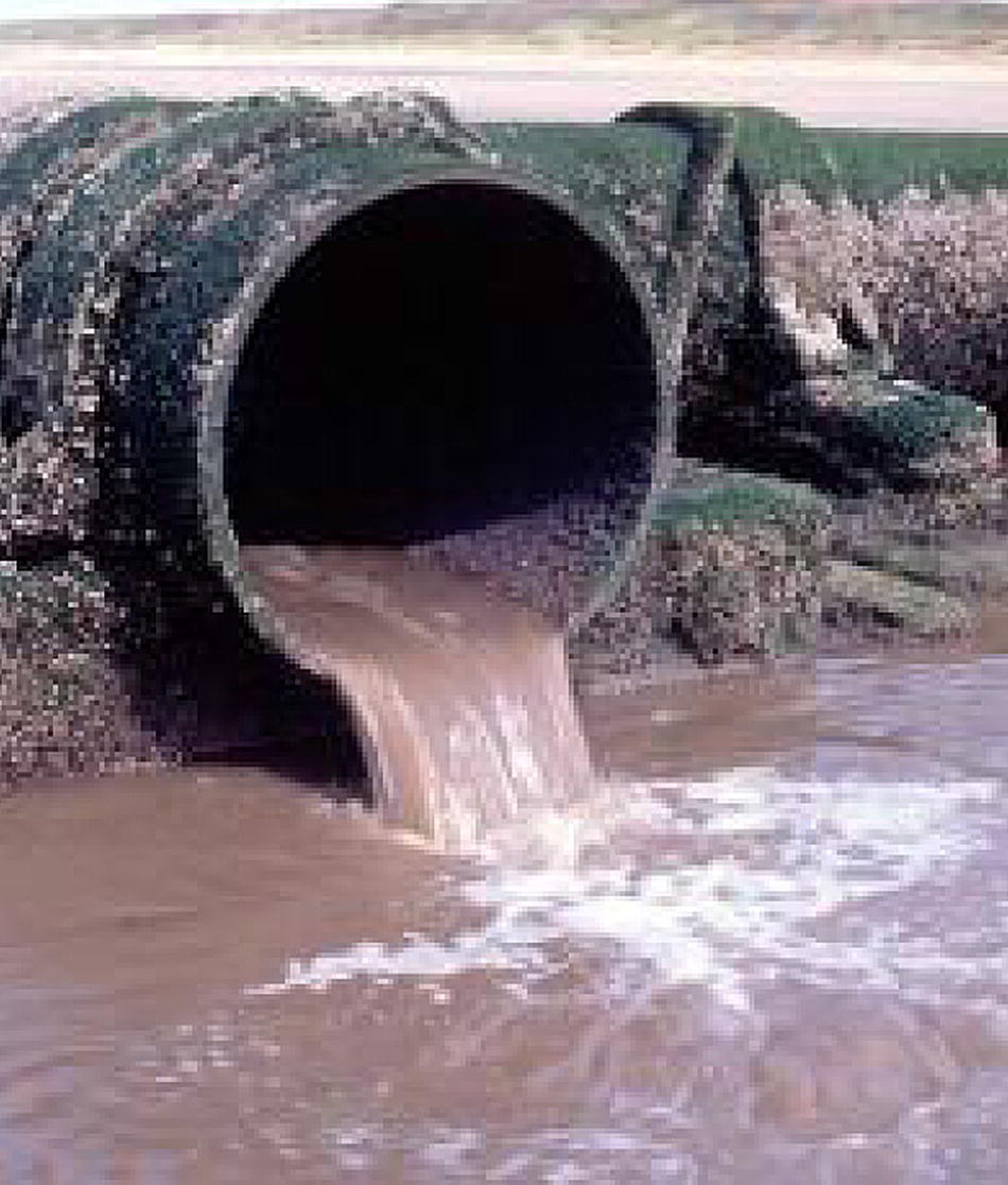
Figure 3.1 Discharge of untreated industrial wastewater to a river.
3.4.5 Some Inorganic Pollutants of Concern
Cyanide ion, CN‐, is probably the most important of the various inorganic species in wastewater. Cyanide, a deadly poisonous substance, exists in water as HCN which is a weak acid. The cyanide ion has a strong affinity for many metal ions, forming relatively less toxic ferrocyanide, Fe(CN)64−, with iron (II), for example. Volatile HCN is very toxic and has been used in gas chamber executions in the United States. Cyanide is widely used in industry, especially for metal cleaning and electroplating. It is also one of the main gas and coke scrubber effluent pollutants from gas works and coke ovens. Cyanide is widely used in certain mineral processing operations.
Ammonia is the initial product of the decay of nitrogenous organic wastes, and its presence frequently indicates the presence of such wastes. It is a normal constituent of some sources of groundwater and is sometimes added to drinking water to remove the taste and odor of free chlorine. Since the pKa (the negative log of the acid ionization constant) of the ammonium ion, NH4+, is 9.26, most ammonia in water is present as NH4+ rather than NH3.
Hydrogen sulphide, H2S, is a product of the anaerobic decay of organic matter containing sulfur. It is also produced in the anaerobic reduction of sulphate by microorganisms and is developed as a gaseous pollutant from geothermal waters. Wastes from chemical plants, paper mills, textile mills, and tanneries may also contain H2S. Nitrite ion, NO2−, occur in water as an intermediate oxidation state of nitrogen. Nitrite is added to some industrial processes to inhibit corrosion; it is rarely found in drinking water at levels over 0.1 mg/l. Sulphite ion, SO32−, is found in some industrial wastewaters. Sodium sulphite is commonly added to boiler feed‐waters as an oxygen scavenger:
3.4.6 Organic Pollutants of Concern
Effluent from industrial sources contains a wide variety of pollutants, including organic pollutants. Primary and secondary sewage treatment processes remove some of these pollutants, particularly oxygen‐demanding substances, oil, grease, and solids. Others, such as refractory (degradation‐resistant) organics (organochlorides, nitro compounds, etc.), salts, and heavy metals, are not efficiently removed. Soaps, detergents, and associated chemicals are potential sources of organic pollutants. Most of the environmental problems currently attributed to detergents do not arise from the surface‐active agents which basically improve the wetting qualities of water. The greatest concern among environmental pollutants has been caused by polyphosphates added to complex calcium functioning as a builder.
Bio‐refractory organics are poorly biodegradable substances, prominent among which are aromatic or chlorinated hydrocarbons (benzene, bornyl alcohol, bromobenzene, chloroform, camphor, dinitrotoluene, nitrobenzene, styrene, etc.). Many of these compounds have also been found in drinking water. Water contaminated with these compounds must be treated using physical and chemical methods, including air stripping, solvent extraction, ozonation, and carbon adsorption.
First discovered as environmental pollutants in 1966, polychlorinated biphenyls (PCB compounds) have been found throughout the world in water, sediments, and in bird and fish tissues. They are made by substituting between 1 and 10 Cl atoms onto the biphenyl aromatic structure. This substitution can produce 209 different compounds (Rouessac and Rouessac 2007).
3.4.7 Thermal Pollution
Considerable time has elapsed since the scientific community and regulatory agencies officially recognized that the addition of large quantities of heat to a recipient possesses the potential of causing ecological harm. The really significant heat loads result from the discharge of condenser cooling water from the ever‐increasing number of steam electrical generating plants and equivalent‐sized nuclear power reactors. Large numbers of power plants currently require approximately 50% more cooling water for a given temperature rise than that required of fossil‐fuel plants of an equal size. The degree of thermal pollution depends on thermal efficiency, which is determined by the amount of heat rejected into the cooling water. Thermodynamically, heat should be added at the highest possible temperature and rejected at the lowest possible temperature if the greatest amount of effect is to be gained and the best thermal efficiency realized. The current and generally accepted maximum operating conditions for conventional thermal stations are about 500 °C and 24 MPa, with a corresponding heat rate of 2.5 kWh, 1.0 kWh resulting in power production and 1.5 kWh being wasted. Plants have been designed for 680 °C and 34 MPa; however, metallurgical problems have kept operating conditions at lower levels.
Nuclear power plants operate at temperatures from 250 to 300 °C and pressures of up to 7 MPa, resulting in a heat rate of approximately 3.1 kWh. Thus, for nuclear plants, 1.0 kWh may be used for useful production, whereas 2.1 kWh is wasted. Most steam‐powered electrical generating plants are operated at varying load factors, and consequently the heated discharges demonstrate wide variation with time. Thus, the biota is not only subjected to increased or decreased temperature, but also to a sudden or “shock,” temperature change. Increased temperature will cause remarkable reduction in the self‐purification capacity of a receiving water body and cause the growth of undesirable algae (Krenkel and Novotny 1980). The addition of heated water to the receiving water can be considered equivalent to the addition of sewage or other organic waste material, since both pollutants may cause a reduction in the oxygen resources of the receiving waters. Also, elevated temperatures in the receiving water could cause undesirable algae bloom (Hauser 2018; USEPA 2018).
3.5 Industrial Wastewater Variation
3.5.1 Pollution Load and Concentration
In most industries, wastewater effluents result from the following water uses:
- Sanitary wastewater (from washing, drinking, etc.)
- Cooling (from disposing of excess heat to the environment)
- Process wastewater (including both water used for making and washing products and for removal and transport of waste and by‐products)
- Cleaning (including wastewater from cleaning and maintenance of industrial areas)
Excluding the large volumes of cooling water discharged by the electric power industry, the wastewater production from urban areas is about evenly divided between industrial and municipal sources. Therefore, the use of water by industry can significantly affect the water quality of receiving waters. The level of wastewater loading from industrial sources varies markedly with the water quality objectives enforced by the regulatory agencies. There are many possible in‐plant changes, process modifications, and water‐saving measures through which industrial wastewater loads can be significantly reduced. Up to 90% of recent wastewater reductions have been achieved by industries employing such methods as recirculation, operation modifications, effluent reuse, or more efficient operation. As a rule, treatment of an industrial effluent is much more expensive without water‐saving measures than the total cost of in‐plant modifications and residual effluent treatment. Industrial wastewater effluents are usually highly variable, with quantity and quality variations brought about by bath discharges, operation start‐ups and shutdowns, working‐hour distribution, and so on. A long‐term detailed survey is usually necessary before a conclusion on the pollution impact from an industry can be reached. Because of the wide variety of industries and levels of pollutants, we can present a snapshot view of the characteristics. The values of typical concentration of conventional pollutants (BOD5, COD, TSS) and pH for different industrial effluents are given in Table 3.3. A similar sampling for nonconventional pollutants is given in Table 3.4.
Table 3.3 Comparative strengths of industrial wastewaters for conventional pollutants.
| Type of waste | BOD5 (mg/l) | COD (mg/l) | TSS (mg/l) | pH |
| Apparel | ||||
| Cotton | 200–1000 | 400–1800 | 200 | 8–12 |
| Wool scouring | 2000–5000 | 2000–5000a | 3 000–30 000 | 9–11 |
| Wool composite | 1 | — | 100 | 9–10 |
| Tannery | 1000–2000 | 2000–4000 | 2 000–3 000 | 11–12 |
| Laundry | 1600 | 2700 | 250–500 | 8–9 |
| Food | ||||
| Brewery | 850 | 1700 | 90 | 4–8 |
| Distillery | 7 | 10 | Low | — |
| Dairy | 600–1000 | — | 200–400 | <7 |
| Agriculture | ||||
| Citrus | 2000 | — | 7 000 | Acid |
| Pea | 570 | — | 130 | <7 |
| Slaughterhouse | 1500–2500 | — | 400–1 000 | 7–8 |
| Potato processing | 2000 | 3500 | 2 500 | 11–13 |
| Sugar beet | 450–2000 | 600–3000 | 800–1 500 | 7–8 |
| Farm | 1000–2000 | — | 1 500–3 000 | 7.5–8.5 |
| Poultry | 500–800 | 600–1050 | 450–800 | 6.5–9 |
| Industries | ||||
| Pulp; sulfite | 1400–1700 | — | Variable | |
| Pulp; kraft | 100–350 | 170–600 | 75–300 | 7–9.5 |
| Paperboard | 100–450 | 300–1400 | 40–100 | |
| Strawboard | 950 | — | 1 350 | |
| Coke oven | 780 | 1650a | 70 | 7–11 |
| Oil refinery | 100–500 | 150–800 | 130–600 | 2–6 |
a COD as KMnO4 mg O2/l.
3.5.2 Industrial Pretreatment
Industrial wastewater may contain pollutants which cannot be removed by conventional sewage treatment. Also, variable flow of industrial waste associated with production cycles may upset the population dynamics of biological treatment units, such as the activated sludge process. Thus, industrial wastewaters can pose serious hazardous to municipal systems because the collection and treatment systems have not been designed to carry or treat them.
Table 3.4 Examples of industrial wastewater concentrations for nonconventional pollutants.
| Industry | Pollutant | Concentration (mg/l) |
| Coke by‐product (steel mill) | Ammonia (as N) | 200 |
| Organic nitrogen (as N) | 100 | |
| Phenol | 2 000 | |
| Metal plating | Chromium (VI) | 3–550 |
| Nylon polymer | COD | 23 000 |
| TOC | 8 800 | |
| Synthetic textile | COD | 3 300 |
| Nitrogen | 40 | |
| Meat processing and packing | COD | 2 100 |
| Nitrogen | 150 | |
| Phosphorus | 16 | |
| Grease | 500 | |
| Temperature | 28 °C | |
| Plywood‐plant glue waste | COD | 2 000 |
| Phenol | 200–2 000 | |
| Phosphorus (as PO4) | 9–15 | |
| Chlorophenolic manufacture | Chloride | 27 000 |
| Phenol | 140 |
Highly regulated industrial effluent usually receives at least pretreatment, if not full treatment, at the factories themselves to reduce the pollutant load, before discharge to the sewer. Using proven treatment technologies and manufacturing practices that promote recycling, industries can remove or eliminate pollutants before discharge of wastewater. This practice is called industrial wastewater treatment or pretreatment.
The pretreatment program is a component of the USEPA (United States Environmental Protection Agency) national NPDES (National Pollutant Discharge Elimination System) program. It is a cooperative effort of federal, state, and local environmental regulatory agencies established to protect water quality. Similar to how USEPA authorizes the NPDES permit program to state, tribal, and territorial governments to perform permitting, administrative, and enforcement tasks for discharges to surface waters (NPDES program), EPA and authorized NPDES state pretreatment programs approve local municipalities to perform permitting, administrative, and enforcement tasks for discharges into the municipalities' POTWs. A treatment works (as defined by CWA section 212) is owned by a state or municipality [as defined by CWA section 502(4)]. This definition includes any devices or systems used in the storage, treatment, recycling, and reclamation of municipal sewage or industrial wastes of a liquid nature. It also includes sewers, pipes, or other conveyances only if they convey wastewater to a POTW treatment plant.
The national pretreatment program identifies specific discharge standards and requirements that apply to sources of nondomestic wastewater discharged to a POTW. By reducing or eliminating waste at the industries (“source reduction”), fewer toxic pollutants are discharged to and treated by the POTW, providing benefits to both the POTWs and the industrial users. Oversight of the program is by the POTW, state, or the EPA. The control authority issues permits for discharge of industrial wastewaters to the POTW. The permits contain numerical limits for controlled pollutants and requirements for sampling, flow measurements, laboratory testing, and reporting.
3.6 Industrial Wastestream Variables
3.6.1 Dilute Solutions
The discharges from continuous manufacturing processes are normally dilute solutions of compatible and sometimes nonconventional pollutants. They may be discharged to the industry's pretreatment system or directly to the POTW without any pretreatment. Manufacturing processes such as plating bath rinses, raw food cleaning, and crude oil dewatering are all examples of dilute solutions of pollutants that may be discharged directly to a POTW sanitary sewer. If a problem occurs in the manufacturing process, a probable result is that the quality of wastewater will change; it may be more laden with pollutants. Some wastestreams from utility services, such as cooling tower and boiler blowdown, are continuous and represent the discharge of dilute solutions.
Another low‐strength wastewater is storm water runoff from chemical handling and storage areas. Products which may have spilled on the industry's grounds are washed off during a rainstorm or during the spring thaw. The pollutant concentration is usually too dilute to require pretreatment before discharge to the sewer, but it exceeds the discharge standards for discharge to surface waters. While the strength of the storm runoff may be low, the volume that must be treated in addition to normal flow to the pretreatment system or to the POTW can cause hydraulic capacity problems. Excessive flows can be diverted to storage reservoirs or basins and then gradually discharged to the pretreatment system. A great deal of attention is presently focused on cleaning up groundwater sources that have been contaminated by leaking underground storage tanks. Cleanup projects of this nature typically involve large quantities of wastes that may contain high concentrations of solvents, fuels, heavy metals, and pesticides. Because of the public attention surrounding groundwater cleanup projects, pretreatment of the contaminated water is almost always required and the result is usually a “high‐ quality” industrial wastewater.
3.6.2 Concentrated Solutions
Typically, concentrated solutions are batch‐generated and the frequency of generation is usually not daily but weekly, monthly, annually, or even longer. These solutions are process chemicals or products that cannot be reconditioned or reused in the same manufacturing process. Concentrated solutions such as spent plating baths, acids, alkalies, static drag out solutions, and reject product may have concentrations of pollutants hundreds or thousands of times higher than the discharge limits of the POTW or higher than can be adequately treated by the pretreatment system if discharged all at once. Time has to be taken to examine and understand each manufacturing process, then identify these concentrated solutions and take the necessary steps to prevent damage to the treatment facilities.
Some wastes may be considered concentrated by the POTW but not by the industry. For example, the 10% sulfuric acid solution used for pickling parts is considered “dilute” by comparison to the 98% or 505 stock solution that the industry uses to make up the pickling solution. When this solution is spent or can no longer be used as a pickling solution, proper treatment and disposal are required. From the industrial manufacturer's point of view, the solution is spent and no longer concentrated. However, from a wastewater treatment point of view, the solution is concentrated since it contains high concentrations of acid (pH < 1.0) and heavy metals (1000 mg/l) compared to the normal pH of 1.0–4.0 and heavy metal concentrations of less than 100 mg/l (IWT 1999). Another source of concentrated solutions is the wastewater from equipment cleanup. While the amount of material in the process chemical bath may be considered dilute by industry standards, it forms a concentrated wastestream when discharged during the cleanup of manufacturing equipment. Cleanup wastestreams contain a high concentration of the product during the first washing of the tank, pipe, or pump. This discharge of concentrated waste is followed by successive rinses which contain less and less pollutants. If cleanup flow concentrations are not equalized, the cleanup cycle can cause problems in the industrial waste treatment system (IWTS). Spills of process chemicals to the floor, if not contained, can flow directly to the floor drain and the pretreatment or sewer system. The adverse effects on the pretreatment system and POTW are the same as those of any other concentrated solutions. This is why chemical containment areas must not have drains.
3.7 Concentration vs. Mass of the Pollution
An understanding of the concentration and the mass of a pollutant in an industrial waste is needed to determine the effects on the industry's pretreatment system, the POTW collection, treatment, and disposal systems, and the sampling of the industry's discharge. The concentration of a substance in wastewater is normally expressed as milligrams per liter and is a measurement of the mass per unit of volume. The mass of a substance is normally expressed in pounds or kilograms and is a weight measurement. A mass discharge rate is a measurement of weight per unit time and is usually expressed as pounds or kilograms per day. Many of the electroplating and all of the metal finishing categorical standards are written in concentrations, whereas most of the other categorical standards are written as mass discharge rate standards. The discharge rate standards recognize that with more production and water, the mass of pollutant will also increase. This approach prevents dilution of the pollutant to meet concentration limitations. The mass discharge rate of a substance can be calculated by knowing the concentration of the pollutant in the wastewater and the volume of wastewater.
The effects of pollutant concentration and mass on the POTW collection, treatment, and disposal systems are generally the same as their effects on the IWTS. However, hydraulic problems in any portion of the POTW system could cause pollutants to pass through the POTW untreated even though the mass of the pollutant did not change. If the daily mass loading is the same, but the instantaneous mass emission rate is highly variable, the POTWs collection system may not equalize the slug loading of a highly concentrated solution. The result may be interference with the treatment system, causing violations of either or both effluent and sludge disposal limitations.
3.7.1 Frequency of Generation and Discharge
Important to both the operation of the industry's pretreatment system and the POTW's collection, treatment, and disposal systems is the frequency of industrial waste generation and discharge. Wastewater sampling to investigate process problems and to determine compliance with the discharge limits are also affected by the hours of discharge.
3.7.2 Hours of Operation vs. Discharge
Normally, the hours of operation are also the hours of discharge to the IWTS. Thus, the operator can generally expect to receive flow for treatment during the hours of operation. If the production is constant, the discharge volume and chemical constituents will also be constant. Several common situations where an industrial waste must be treated after the normal production hours are described below:
- The “wet” processes run for one shift, but the “dry” processes run for two. The dry processes may require utilities such as compressed air or a boiler, each having a wastewater discharge.
- In industries with long collection systems, production and wastewater flow to the system may stop, but the IWTS may continue to operate and discharge until the wastewater in the collection system has been processed.
- Spills, accidental discharges, or storm water flow that goes to the IWTS may cause the IWTS to operate outside of the normal production hours.
- A food‐processing plant operates for one or two shifts, generating some wastewater, but most of the equipment cleaning operations occur on an off shift. The cleaning generates most of the wastewater volume.
- The IWTS has an equalization tank either at the beginning of the IWTS or at the end of the manufacturing system. Discharge from the equalization tank to the rest of the IWTS may continue after production stops because it is programmed to pump to the next unit process until it reaches its low level.
Equalization of the wastewater is an important factor affecting the actual hours of wastewater discharge to the IWTS and sewer. In order to deliver a relatively constant flow and concentration of pollutants to the IWTS, large wastewater collection sumps, equalization tanks, or storage tanks may be used. As noted above, these equalization devices may also lengthen the time of discharge beyond the actual hours of operation of the manufacturing facility. Equalization of industrial wastewater flows can also be beneficial to the POTW. By lengthening the hours of discharge from the industry, there is an effective increase in the available hydraulic capacity of the POTW collection system because of the decreased industrial flow rates. Due to the normal diurnal variation in domestic wastewater flows (peak flows usually occur between 8 : 00 a.m. and 6 : 00 p.m.), the hydraulic capacity of a sewer may be exceeded if a large industrial flow is allowed to be discharged to the sewer during a short period. Therefore, it may be necessary for the industry to discharge only at night. Sampling of this discharge would then be shifted to the night‐time hours.
3.7.3 Discharge Variations
Industries that have daily, weekly, or seasonal manufacturing cycles will show variations in wastewater generation. Business cycles for each of the various segments of the industrial community will have an effect on production; therefore, on the generation of wastewater. The food‐processing industry provides a good example of daily, weekly, and seasonal variations in discharge quantity and quality. For example, an industry that processes citrus peel to make pectin is dependent on when the peel arrives at the industry's plant. This may mean anywhere from three to six days per week. As the season progresses, the type of peel changes from orange to lemon and the sugar content changes yielding a slightly different type of wastewater. After the citrus season, the plant is completely shut down. In certain industries, variations in the quantity of wastewater reflect the nature of the business or the business cycle of the particular business segment. In a small shop producing printed circuit boards, it is typical to have a 30‐day turnaround with sales, ordering, and development taking place during the first part of the month. Production is slow while making test boards, but once the board is developed, production proceeds at a rapid pace to produce the boards for shipment in the last week of the month. The printed circuit board industry is subject to both downturns and upturns in the market. The major pollutant from the industry is copper, consequently, the quantity of copper discharged to the industrial sewer fluctuates according to market and production cycles.
Variations in the quality of industrial waste can also occur due to market forces or environmental concerns requiring a different type of product. In the metal‐finishing industry, for example, companies are moving from cadmium‐plated metal, an environmentally more hazardous substance with more stringent discharge limitations, to zinc‐plated parts. Knowledge of the industry, the manufacturing processes, and market forces are valuable tools needed by the industrial waste treatment plant operator to anticipate variations in industrial discharges.
3.7.4 Continuous and Intermittent Discharges
Discharges from manufacturing facilities usually reflect the type of manufacturing process used at the facility. Processes which are continuous tend to produce wastewater on a continuous basis with relatively constant volume and quality. Batch processes or activities that occur once per shift, per day, or per week tend to produce an intermittent discharge. Also, as a general rule‐of‐thumb, the larger the manufacturing process, the more likelihood there is of a continuous discharge. Examples of manufacturing processes that have continuous discharges include rinsing or cleaning of parts or food, processing of crude oil, either at the well head or refinery, air or fume scrubbing, papermaking, and leather tanning. Intermittent discharges of wastewater are characterized by discharges of a volume of wastewater separated by a time period between discharges.
These typically occur at the beginning or ending of a manufacturing process or during equipment cleanup, a spill, replacement of spent solution, or disposal of a rejected product. Intermittent discharges also tend to be more concentrated and of smaller volume than the wastewater normally discharged. For an industrial pretreatment facility, the intermittent discharges and the variations in waste generation determine the design capacity of the system.
3.7.5 Industrial Effluents
Whereas the nature domestic wastewater is relatively constant, the extreme diversity of industrial effluents calls for an individual investigation for each type of industry and often entails the use of specific treatment processes. Therefore, a thorough understanding of the production processes and the system organization is fundamental.
There are four types of industrial effluents to be considered:
- General manufacturing effluents: Most processes give rise to polluting effluents resulting from the contact of water with gases, liquids, or solids. The effluents are either continuous or intermittent. They even might only be produced several months a year (campaigns in the agriculture and food industry, two months for beet sugar production, for example). Usually, if production is regular, pollution flows are known. However, for industries working in specific campaigns (synthetic chemistry, pharmaceutical and allied chemical industries), it is more difficult to analyze the effluents as they are always changing.
- Specific effluents: Some effluents are likely to be separated either for specific treatment after which they are recovered, or to be kept in a storage tank ready to be reinjected at a weighted flow rate into the treatment line, such as pickling and electroplating baths, or spent caustic soda.
- General service effluents: These effluents may include wastewater (canteens, etc.), water used for heating (boiler blowdown, spent resin regenerants), etc.
- Intermittent effluents: These must not be forgotten; they may occur from accidental leaks of products during handling or storage, from floor wash water and from polluted water, of which storm water may also give rise to a hydraulic overload.
For the correct design of an industrial effluent treatment plant, the following parameters must be carefully established (IWT 1999):
- Types of production, capacities and cycles, raw materials used
- Composition of the make‐up water used by the industrial plant
- Possibility of separating effluents and/or recycling them
- Daily volume of effluents per type
- Average and maximum hourly flows (duration and frequency by, type)
- Average and maximum pollution flow (frequency and duration) per type of waste and for the specific type of pollution coming from the industry under consideration, since it can seriously disturb the working of certain parts of the treatment facilities (glues, tars, fibers, oils, sands, etc.)
In the starch industry, starch is extracted from tubers of manioc and potatoes. A wet process is used to extract starch from the richest cereals (wheat, rice, corn). The general pollution of this process is shown in Table 3.5. The nature of the effluents depends on the specific treatments used on the raw materials after common washing.
The effluents are rather acidic which is due to lactic fermentation or to sulphitation process in white sugar manufacture (pH 4–5). When a wet technique is used to extract starch, the pollution comes from the evaporation of water and it is made up of volatile organic acids. A notably soluble protein‐rich pollution may come from the glucose shop. The general wastes of potatoes processing is presented in Table 3.6.
3.7.6 Wastewater Quality Indicators: Selected Pollution Parameters
3.7.6.1 Solids
Solid material in wastewater may be dissolved, suspended, or settled. Total dissolved solids or TDS (sometimes called filterable residue) is measured as the mass of residue remaining when a measured volume of filtered water is evaporated. The term total suspended solids (TSS) refers to the nonfilterable residue that is retained on a glass‐fiber disc after filtration of a sample of wastewater. Settleable solids are measured as the visible volume accumulated at the bottom of an Imhoff cone after water has settled for one hour. Turbidity is a measure of the light‐scattering ability of suspended matter in the water. Salinity measures water density or conductivity changes caused by dissolved materials.
Table 3.5 General pollution of wet process for starch producing.
| Raw material | Volume of water (m3/T) | BOD5 (kg/T) |
| Corn starch | 2–4 | 5–12 |
| Rice starch | 8–12 | 5–10 |
| Wheat starch (gravity separation) | 10–12 | 40–60 |
Table 3.6 Potato processing wastes.
| Facility or shop | Volume of water (m3/T) | SS (kg/T) | BOD5 (kg/T) |
| Preparation | |||
| Transport and washing | 2.5–6 recyclable | 20–200 | — |
| Peeling and cutting | 2–3 | — | 5–10 |
| Flakes | |||
| Bleaching and cooking | 2–4 | — | 10–15 |
| Crisps | |||
| Bleaching | 2.2–5 | 5–10 | 5–15 |
| Starch extractiona | |||
| Washing, grating, grinding | 2–6 (Red water) | Recyclable pulp | 20–60b |
| Pressing – refining | 1 |
a International Starch Institute Aarhus Denmark Potato Starch Effluents.
b Including preparation water.
3.7.6.2 Oxygen
Most aquatic habitats are occupied by fish or other animals requiring certain minimum dissolved oxygen concentrations to survive. Dissolved oxygen concentrations may be measured directly in wastewater, but the amount of oxygen potentially required by other chemicals in the wastewater is termed as oxygen demand. Dissolved or suspended oxidizable organic material in wastewater will be used as a food source. Finely divided material is readily available to microorganisms whose populations will increase to digest the amount of food available. Digestion of this food requires oxygen, so the oxygen content of the water will ultimately be decreased by the amount required to digest the dissolved or suspended food. Oxygen concentrations may fall below the minimum required by aquatic animals if the rate of oxygen utilization exceeds replacement by atmospheric oxygen.
Basically, the reaction for biochemical oxidation may be written as
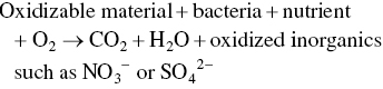
Oxygen consumption by reducing chemicals such as sulfides and nitrites is typified as follows:
3.7.6.3 Biochemical and Chemical Oxygen Demands
The most widely used parameter of organic pollution applied to both wastewater and surface water is the five‐day biochemical oxygen demand (BOD5).
This determination involves the measurement of the dissolved oxygen used by microorganisms in the biochemical oxidation of organic matter in a five‐day period. The total amount of oxygen consumed when the biochemical reaction is allowed to proceed to completion is called the ultimate BOD. Because the ultimate BOD is so time‐consuming, the BOD5 has been almost universally adopted as a measure of relative pollution effect.
3.7.6.4 COD
COD is widely used to characterize the organic strength of wastewaters and pollution of natural of natural waters. The test measures the amount of oxygen required for chemical oxidation of organic matter in the sample to carbon dioxide and water.
Both the BOD and COD tests are a measure of the relative oxygen‐depletion effect of a waste contaminant. Both have been widely adopted as a measure of pollution effect. The BOD test measures the oxygen demand of biodegradable pollutants, whereas the COD test measures the oxygen demand of biodegradable pollutants plus the oxygen demand of non‐biodegradable oxidizable pollutants.
3.7.6.5 Nitrogen
Nitrogen is an important nutrient for plant and animal growth. Atmospheric nitrogen is less biologically available than dissolved nitrogen in the form of ammonia and nitrates. Availability of dissolved nitrogen may contribute to algal blooms. Ammonia and organic forms of nitrogen are often measured as total Kjeldahl nitrogen, and analysis for inorganic forms of nitrogen may be performed for more accurate estimates of total nitrogen content.
3.7.6.6 Phosphates
Phosphates enter the water ways through both NPSs and point sources. NPS pollution refers to water pollution from diffuse sources. NPS pollution can be contrasted with point source pollution where discharges occur to a body of water at a single location. The NPSs of phosphates include natural decomposition of rocks and minerals, storm water runoff, agricultural runoff, erosion and sedimentation, atmospheric deposition, and direct input by animals/wildlife, whereas point sources may include wastewater treatment plants and permitted industrial discharges. In general, the NPS pollution typically is significantly higher than the point sources of pollution. Therefore, the key to sound management is to limit the input from both point sources and NPSs of phosphate. High concentration of phosphate in water bodies is an indication of pollution and largely responsible for eutrophication.
3.7.6.7 Pollutant Concentration and Loading in Wastewater
Loadings on wastewater treatment units are often expressed in terms of pounds of BOD or TSS per day or pounds of solids per day, as well as quantity of flow per day. The relationship between the parameters of concentration and flow is based on the following conversion factors: 1.0 mg/l, which is also 1.0 parts per million (ppm) by weight, equals 8.34 or 62.4 lb/million gal (MG), since 1 gal of water weighs 8.34 lb.
Conversion of mg/l (ppm) to lb/MG

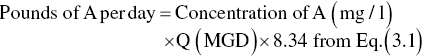
or
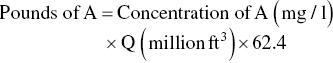
where
- A = BOD, TSS, or other constituents (mg/l)
- Q = volume of wastewater (MG or million ft3)
- 8.34 = (lb/MG)/(mg/l)
- 62.4 = (lb/million ft3)/(mg/l)
3.8 Industrial Wastewater Treatment
3.8.1 Variation in Industrial Wastewaters
The composition of wastewater from industry operations varies widely depending on the function and activity of the particular industry (Tables 3.3 and 3.4). From these examples, it can be observed that the daily average concentration of both BOD and TSS can vary significantly. Problems with high short‐term loadings most commonly occur in small treatment plants that have limited reserve capacity to handle “shock loadings.” If industrial wastes are to be discharged to the collection system for treatment in a POTW, it will be necessary to characterize the wastes adequately to identify the ranges in constituent concentrations and mass loadings. Such characterization is also needed to determine if pretreatment is required before the waste is permitted to be discharged into the POTW collection system. If pretreatment is needed, the effluent from the pretreatment facilities must also be characterized. Further, any proposed future process changes should also be assessed to determine what effects they might have on the wastes to be discharged.
3.8.2 Pretreatment Program Purpose
The purpose of the USEPA National Pretreatment Program is to protect POTWs and the environment from the adverse impacts that may occur when “shock loadings” of criteria pollutants or hazardous or toxic wastes are discharged into a POTW system. This is achieved mainly by regulating nondomestic (industrial) users of POTWs that discharge toxic wastes or unusually strong conventional wastes. The Federal Water Pollution Control Act, known as the Clean Water Act (CWA), was passed in 1972 to maintain and improve the quality of ambient waters. Its goal was to eliminate the introduction of pollutants into navigable waters and to achieve fishable and swimmable water quality. The NPDES and its permit programs establish requirements for point source direct dischargers to the water environment. The National Pretreatment Program, a component of NPDES, requires indirect industrial and commercial waste dischargers, or those that discharge wastewater to a POTW, to obtain permits that specify the effluent quality to be obtained by pretreatment or other controls before discharge to POTW systems. Thus, the CWA gives the EPA the authority to establish and enforce pretreatment standards for discharge of industrial wastewaters into POTW facilities.
3.8.2.1 Pretreatment Specific Goals
- To prevent the introduction of pollutants into POTWs which will interfere with the operation of the POTW, including interference with its use or disposal of municipal sludge.
- To prevent the introduction of pollutants into POTWs which pass through the treatment works into the receiving waters or cause upsets to the treatment works.
- To protect the sludge quality and improve the possibility of recycle and reuse of municipal and industrial wastewaters.
- To reduce the health and environmental risk of pollution by the discharge of toxic pollutants into the collection system and POTW.
3.8.3 Dental Waste Pretreatment Management
Dental offices create a variety of wastes, which need to be pretreated or managed correctly to protect our health and the environment. This guide explains the Best Management Practices (BMPs) that will help dentists follow environmental laws and prevent pollution. Note that this guidance is only for dental offices on a POTW. Operatory waste should never go to a septic system or POTW, even with an amalgam separator.
Dental amalgam waste is a significant source of mercury received by POTWs and they can't treat the mercury in waste, so it pollutes natural water bodies and the land the solids are applied to. For more information, consult the American Dental Association's Dental Amalgam BMPs.
On 15 December 2016, EPA Administrator signed the final rule related to dental categorical standards, and the EPA submitted the rule for publication in the Federal Register. The official version of the rule for purposes of compliance has been presented in a Federal Register publication. The publication rule can be found at https://www.epa.gov/eg/dental‐effluent‐guidelines‐documents.
3.9 Air Quality
The terms ambient air, ambient air pollution, ambient levels, ambient concentrations, ambient air monitoring, ambient air quality, etc. occur frequently in air pollution parlance. The intent is to distinguish pollution of the air outdoors by transport and diffusion by wind (i.e. ambient air pollution) from contamination of the air indoors by the same substances.
The air inside a factory building can be polluted by release of contaminants from industrial processes to the air of the workroom. This is a major cause of occupational disease. Prevention and control of such contamination are part of the practice of industrial hygiene. To prevent exposure of workers to such contamination, industrial hygienists use industrial ventilation systems that remove the contaminated air from the workroom and discharge it, either with or without treatment to remove the contaminants to the ambient air outside the factory building.
The air inside a home, office, or public building is the subject of much interest and is referred to as indoor air pollution or indoor air quality. These interior spaces may be contaminated by such sources as fuel‐fired cooking or space‐heating ranges, ovens, or stoves that discharge their combustion products to the room; by solvents evaporated from inks, paints, adhesives, cleaners, or other products; by formaldehyde, radon, and other products emanating from building materials; and by other pollutant sources indoors. If some of these sources exist inside a building, the pollution level of the indoor air might be higher than that of the outside air. However, if none of these sources are inside the building, the pollution level inside would be expected to be lower than the ambient concentration outside because of the ability of the surfaces inside the building – walls, floors, ceilings, furniture, and fixtures – to adsorb or react with gaseous pollutants and attract and retain particulate pollutants, thereby partially removing them from the air breathed by occupants of the building. This adsorption and retention would occur even if doors and windows were open, but the difference between outdoor and indoor concentrations would be even greater if they were closed, in which case air could enter the building only by infiltration through cracks and walls.
Many materials used and dusts generated in buildings and other enclosed spaces are allergenic to their occupants. Occupants who do not smoke are exposed to tobacco and its associated gaseous and particulate emissions from those who do. This occurs to a much greater extent indoors than in the outdoor air. Many ordinances have been established to limit or prohibit smoking in public and workplaces. Attempts have been made to protect occupants of schoolrooms from infections and communicable diseases by using ultraviolet (UV) light or chemicals to disinfect the air. These attempts have been unsuccessful because disease transmission occurs instead outdoors and in unprotected rooms. There is, of course, a well‐established technology for maintaining sterility in hospital operating rooms and for manufacturing operations in pharmaceutical and similar plants.
Figure 3.2 The regions of the atmosphere
3.9.1 The Atmosphere
On a mesoscale (Figure 3.2) as temperature varies with altitude, so does density. In general, the air grows progressively less dense as we move upward from the troposphere through the stratosphere and the chemosphere to ionosphere. In the upper reaches of the ionosphere, the gaseous molecules are few and far between as compared with the troposphere.
The ionosphere and chemosphere are of interest to space scientists because they must be traversed by space vehicles en route to or from the moon or the planets, and they are regions in which satellites travel in the Earth's orbit. These regions are of interest to communications scientists because of their influence on radio communications and they are of interest to air pollution scientists primarily because of their absorption and scattering of solar energy, which influences the amount and spectral distribution of solar energy and cosmic rays reaching the stratosphere and troposphere.
The stratosphere is of interest to aeronautical scientists because it is traversed by airplanes; to communications scientists because of radio and television communications; and to air pollution scientists because global transport of pollution, particularly the debris of aboveground atomic bomb tests and volcanic eruptions occur in this region and because absorption and scattering of solar energy also occur there. The lower portion of this region contains the stratospheric ozone layer which absorbs harmful UV solar radiation. Global change scientists are interested in modifications of this layer by long‐term accumulation of chlorofluorocarbons and other gases released at the Earth's surface or by high‐altitude aircraft.
The troposphere is the region in which we live and is the primary focus of this book.
3.9.2 Unpolluted Air
The gaseous composition of unpolluted tropospheric air is given in Table 3.7. Unpolluted air is a concept, i.e., what the composition of the air would be if humans and their works were not on Earth. We will never know the precise composition of unpolluted air because by the time we had the means and the desire to determine its composition, humans had been polluting the air for thousands of years. Now even at the most remote locations at sea, at the poles, and in the deserts and mountains, the air may be best described as dilute polluted air. It closely approximates unpolluted air, but differs from it to the extent that it contains vestiges of diffused and aged human‐made pollution.
The real atmosphere is more than a dry mixture of permanent gases. It has other constituents‐vapor of both water and organic liquids and particulate matter held in suspension. Above their temperature of condensation, vapor molecules act just like permanent gas molecules in the air. The predominant vapor in the air is water vapor. Below its condensation temperature, if the air is saturated, water changes from vapor to liquid. We are all familiar with this phenomenon because it appears as fog or mist in the air and as condensed liquid water on windows and other cold surfaces exposed to air. The quantity of water vapor in the air varies greatly from almost complete dryness to super‐saturation, i.e., between 0 and 4% by weight. Gaseous composition in Table 3.7 is expressed as parts per million by volume – ppm (vol) (when a concentration is expressed simply as ppm).
3.9.3 Mobile Sources and Emission Inventory
Generally, mobile sources imply transportation, but sources such as construction, equipment, gasoline‐powered lawn mowers, and gasoline‐powered tools are included in the category. Mobile sources, therefore, consists of many different types of vehicles powered by engines using different cycles, fueled by a variety of products and emitting varying amounts of both simple and complex pollutants. The emissions from a gasoline‐powered vehicle come from many sources. With most of today's automobiles using unleaded gasoline, lead emissions are no longer a major concern.
An emission inventory is a list of the amount of pollutants from all sources entering the air in a given time period. The boundaries of the area are fixed. The emission inventories are very useful to control agencies as well as planning and zoning agencies. They can point out the major sources whose control can lead to a considerable reduction of pollution in the area. They can be used with appropriate mathematical models to determine the degree of overall control necessary to meet ambient air quality standards. They can be used to indicate the type of sampling network and the locations of individual sampling stations if the areas chosen are small enough. For example, if an area uses very small amounts of sulfur‐bearing fuels, establishing an extensive SO2 monitoring network in the area would not be an optimum use of public funds. Emission inventories can be used for publicity and political purposes: “If natural gas cannot meet the demands of our area, we will have to burn more high‐sulfur fuel, and the SO2 emissions will increase by 8 tons per year.”
The method used to develop the emission inventory does have some elements of error, but the other two alternatives are expensive and subject to their own errors. The first alternative would be to monitor continually every major source in the area. The second method would be to monitor continually the pollutants in the ambient air at many points and apply appropriate diffusion equations to calculate the emissions. In practice, the most informative system would be a combination of all three, knowledgeably applied.
The US Clean Air Act Amendments of 1990 (CAAA) strengthened the emission inventory requirements for plans and permits in non‐attainment areas. The amendments state:
INVENTORY – Such plan provisions shall include a comprehensive, accurate, current inventory of actual emissions from all sources of the relevant pollutant or pollutants in such area, including such periodic revisions as the Administrator may determine necessary to assure that the requirements of this part are met.
IDENTIFICATION AND QUANTIFICATION – Such plan provisions shall expressly identify and quantify the emissions, if any, of any such pollutant or pollutants which will be allowed, from the construction and operation of major new or modified stationary sources in each such area. The plan shall demonstrate to the satisfaction of the Administrator that the emissions quantified for this purpose will be consistent with the achievement of reasonable further progress and will not interfere with the attainment of the applicable national ambient air quality standard by the applicable attainment date.
3.9.4 Inventory Techniques
To develop an emission inventory for an area, one must (i) list the types of sources for the area, such as furnaces, automobiles, and home fireplaces; (ii) determine the type of air pollutant emission from each of the listed sources, such as particulates and SO2; (iii) examine the literature to find valid emission factors for each of the pollutants of concern (e.g. “particulate emissions for open burning of waste wood or sawdust are 10 kg per ton of residue consumed”); (iv) through an actual count, or by means of some estimating technique, determine the number and size of specific sources in the area (the number of steelmaking furnaces can be counted, but the number of home fireplaces will probably have to be estimated); and (v) multiply the appropriate numbers from (iii) and (iv) to obtain the total emissions and then sum the similar emissions to obtain the total for the area.
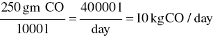
A typical example will illustrate the procedure. Suppose we wish to determine the amount of carbon monoxide from oil furnaces emitted per day, during the heating season, in a small city of 50 000 population:
Table 3.7 The gaseous composition of unpolluted air (dry basis).
| ppm (vol) | μg/m3 | |
| Nitrogen | 780 000 | 8.95 × 10⁸ |
| Oxygen | 209 400 | 2.74 × 10⁸ |
| Water | — | — |
| Argon | 9 300 | 1.52 × 10⁷ |
| Carbon dioxide | 315 | 5.67 × 10⁵ |
| Neon | 18 | 1.49 × 10⁴ |
| Helium | 5.2 | 8.50 × 10² |
| Methane | 1.0–1.2 | 6.56–7.87 × 10² |
| Krypton | 1.0 | 3.43 × 10³ |
| Nitrous oxide | 0.5 | 9.00 × 10² |
| Hydrogen | 0.5 | 4.13 × 101 |
| Xenon | 0.08 | 4.29 × 10² |
| Organic vapors | 0.02 | — |
- The source is oil furnaces within the boundary area of the city.
- The pollutant of concern is carbon monoxide.
- Emission factors for carbon monoxide are listed in various ways (240 gm/1000 l of fuel oil, 50 gm/day/burner, 1½% by volume of exhaust gas, etc.). For this example, use 240 gm/1000 l of fuel oil.
Fuel oil sales figures, obtained from the local dealers association, average 40 000 l/day.
3.9.5 Data Reduction and Compilation
The final emission inventory can be prepared on a computer. This will enable the information to be stored on magnetic tape or disk so that it can be updated rapidly and economically as new data or new sources appear. The computer program can be written so that changes can easily be made. There will be times when major changes occur and the inventory must be completely changed. Imagine the change that would take place when natural gas first becomes available in a commercial‐residential area which previously used oil and coal for heating.
To determine emission data, as well as the effect that fuel changes would produce, it is necessary to use the appropriate thermal conversion factor from one fuel to another. Table 3.2 lists these factors for fuels in common use.
A major change in the emissions for an area will occur if control equipment is installed. This can be shown in the emission inventory to illustrate the effect on the community.
By keeping the emission inventory current and updating it at least yearly as fuel uses change, industrial and population changes occur and control equipment is added, a realistic record for the area is obtained.
3.9.6 Major Sources of Air Emissions
3.9.6.1 US Clean Air Act and Amendments
The Clean Air Act (CAA) defines the national policy for air pollution abatement and control in the United Kingdom. It establishes goals for protecting health and natural resources and delineates what is expected of Federal, State, and local governments to achieve those goals. The CAA, which was initially enacted as the Air Pollution Control Act of 1955, has undergone several revisions over the years to meet the ever‐changing needs and conditions of the nation's air quality. Though it is the intent of Congress to reauthorize and update by amendment all major federal legislation on a five‐year schedule, disagreements over policies related to the control of acidic deposition contributed to an eight‐year hiatus in amending the CAA. In 1900, major agreements on clean air amendments were reached by members of Congress and the president. The 1990 CAAA represented a significant political achievement. Major new or expanded authorities included changes in the timetables for the achievement of air‐quality standards in non‐attainment areas, the regulation of emissions from motor vehicle, regulation of hazardous air pollutants (HAPs), acidic deposition control, stratospheric O3, protection, permitting requirements, and enforcement.
3.9.7 1990 Clean Air Act Amendments
On 15 November 1990, the President signed the amendments to the CAA, referred to as the 1990 CAAA. Embodied in these amendments were several progressive and creative new themes deemed appropriate for effectively achieving the air quality goals and for reforming the air quality control regulatory process (USEPA 1990). Specifically, the amendments:
- Encouraged the use of market‐based principles and other innovative approaches similar to performance‐based standards and emission banking and trading.
- Promoted the use of clean low‐sulfur coal and natural gas, as well as innovative technologies to clean high‐sulfur coal through the acid rain program.
- Reduced energy waste and created enough of a market for clean fuels derived from grain and natural gas to cut dependency on oil imports by over million barrels per day.
- Promoted energy conservation through an acid rain program that gave utilities flexibility to obtain needed emission reductions through programs that encouraged customers to conserve energy.
3.9.8 Introduction to Air Pollution Control and Estimating Air Emission Rates
Air pollution control has become an essential part of operations for many industries particularly the chemical process industries. In developed countries, air quality problems are attributable to the by‐products of combustion processes used in the private and public transportation sectors of the economy, as well.
Frequently; however, planners fail to acknowledge that control systems themselves are industrial processes that consume energy and can emit significant amounts of pollutants into the atmosphere. Regulators have tended to pursue the control of each target pollutant independently with little consideration of secondary pollutants.
In the United States, for example, regulation of air pollution started with the largest sources because they had the most potential for immediate environmental improvement and because the major corporations responsible for these sources could reasonably be asked to assimilate the costs of added controls. The next regulatory phase saw a progressive tightening of standards and application of limits to more and smaller sources, with priority pollutants targeted as separate and distinct entities to be controlled.
3.9.8.1 Air Emission Estimates
It is critical for a facility to make realistic estimates of the emissions it produces, which will help in determining compliance, predicting potential public exposure and health impacts and designing effective air pollution control equipment or strategies (Karell 2017).
3.9.8.2 Emission Factors
Valid emission factors for each source of pollution are the key to the emission inventory. It is not uncommon to find emission factors differing by 50%, depending on the researcher, variables at the time of emission measurement, etc. Since it is possible to reduce the estimating errors in the inventory to ±10% by proper statistical sampling techniques, an emission factor error of 50% can be overwhelming. It must also be realized that an uncontrolled source will emit at least 10 times the amount of pollutants released from one operating properly with air pollution control equipment installed.
Actual emission data are available from many handbooks, government publications, and literature searches of appropriate research papers and journals. It is always wise to verify the data, if possible, as to the validity of the source and the reasonableness of the final number. Some emission factors, which have been in use for years, were only rough estimates proposed by someone years ago to establish the order of magnitude of the particular source.
Emission factors must be also critically examined to determine the tests from which they were obtained. For example, carbon monoxide from an automobile will vary with the load, engine speed, displacement, ambient temperature, coolant temperature, ignition timing, carburetor adjustment, engine condition, etc. However, in order to evaluate the overall emission of carbon monoxide to an area, we must settle on an average value that we can multiply by the number of cars, or kilometers driven per year, to determine the total carbon monoxide released to the area.
Published emission factors are available in the literature for many process situations and types of equipment. These are often calculated and published by the USEPA and other agencies, equipment vendors, and trade associations. Many of these emission factors are published in normalized terms, such as pounds of contaminant per 1000 gal of certain fuel combusted, pounds per kilowatt of electricity produced, etc. Manufacturers often provide an emission factor as a guarantee, which enables the user to estimate the emissions from the equipment and obtain a permit for the unit.
Compilation of air pollutant emissions factors (AP‐42) (Table C.1) and emission inventories have long been fundamental tools for air quality management (USEPA 1995). Emission estimates are important for developing emission control strategies, determining applicability of permitting and control programs, ascertaining the effects of sources and appropriate mitigation strategies, plus a number of other related applications by an array of users including federal, state, local agencies, consultants, and industry. Data from source‐specific emission tests or continuous emission monitors are usually preferred for estimating a source's emissions because those data provide the best representation of the tested source's emissions. However, test data from individual sources are not always available and, even then, they may not reflect the variability of actual emissions over time. Thus, emission factors are frequently the best or only method available for estimating emissions, in spite of their limitations.
The passage of the Clean Air Act Amendments of 1990 (CAAA) and the Emergency Planning and Community Right‐to‐Know Act (EPCRA) of 1986 has increased the need for both criteria and HAP emission factors and inventories. The Emission Factor and Inventory Group (EFIG), in the USEPA's Office of Air Quality Planning and Standards, develops and maintains emission estimating tools to support the many activities mentioned above. The AP‐42 series is the principal means by which EFIG can document its emission factors. These factors are cited in numerous other EPA publications and electronic data bases, but without the process details and supporting reference material provided in AP‐42.
3.9.8.3 What Is an AP‐42 Emission Factor?
An emission factor is a representative value that attempts to relate the quantity of a pollutant released to the atmosphere with an activity associated with the release of that pollutant. These factors are usually expressed as the weight of pollutant divided by a unit weight, volume, distance, or duration of the activity emitting the pollutant (e.g. kilograms of particulate emitted per megagram of coal burned). Such factors facilitate estimation of emissions from various sources of air pollution. In most cases, these factors are simply averages of all available data of acceptable quality and are generally assumed to be representative of long‐term averages for all facilities in the source category (i.e. a population average).
The general equation for emission estimation is
where
- E = emissions,
- A = activity rate,
- EF = emission factor, and
- ER = overall emission reduction efficiency, %.
ER is further defined as the product of the control device destruction or removal efficiency and the capture efficiency of the control system. When estimating emissions for a long time period (e.g. one year) both the device and the capture efficiency terms should account for upset periods as well as routine operations.
3.9.8.4 AP‐42 by Chapters: Emission Factors for Quantifications
AP‐42, Compilation of Air Pollutant Emission Factors, has been published since 1972 as the primary compilation of EPA's emission factor information. It contains emission factors and process information for more than 200 air pollution source categories. A source category is a specific industry sector or group of similar emitting sources. The emission factors have been developed and compiled from source test data, material balance studies, and engineering estimates. The fourth edition of AP‐42 was published in 1995 (USEPA 1985a). Since then EPA has published supplements and updates to the 15 chapters available in Volume I, Stationary Point and Area Sources. Use the AP‐42 Chapter webpage links to access the document by chapter (Table C.2).
Emission factor ratings in AP‐42 (discussed below) provide indications of the robustness, or appropriateness of emission factors for estimating average emissions for a source activity. Usually, data are insufficient to indicate the influence of various process parameters such as temperature and reactant concentrations. For a few cases, however, such as in estimating emissions from petroleum storage tanks, this document contains empirical formulae (or emission models) that relate emissions to variables such as tank diameter, liquid temperature, and wind velocity. Emission factor formulae that account for the influence of such variables tend to yield more realistic estimates than would factors that do not consider those parameters.
The extent of completeness and detail of the emissions information in AP‐42 is determined by the information available from published references. Emissions from some processes are better documented than others. For example, several emission factors may be listed for the production of one substance: one factor for each of a number of steps in the production process such as neutralization, drying, distillation, and other operations. However, because of less extensive information, only one emission factor may be given for production facility releases for another substance, though emissions are probably produced during several intermediate steps. There may be more than one emission factor for the production of a certain substance because differing production processes may exist or because different control devices may be used. Therefore, it is necessary to look at more than just the emission factor for a particular application and to observe details in the text and in table footnotes.
The fact that an emission factor for a pollutant or process is not available from USEPA does not imply that the Agency believes the source does not emit that pollutant or that the source should not be inventoried, but it is only that USEPA does not have enough data to provide any advice.
Emission factors may be appropriate to use in a number of situations such as making source‐specific emission estimates for area wide inventories. These inventories have many purposes, including ambient dispersion modeling and analysis, control strategy development, and in screening sources for compliance investigations. Emission factor use may also be appropriate in some permitting applications such as in applicability determinations and in establishing operating permit fees.
Emission factors in AP‐42 are neither USEPA‐recommended emission limits (e.g. best available control technology or BACT or maximum achievable control technology or MACT or lowest achievable emission rate or LAER) nor standards (e.g. National Emission Standard for Hazardous Air Pollutants or NESHAP or New Source Performance Standards or NSPS). Use of these factors as source‐specific permit limits and/or as emission regulation compliance determinations is not recommended by USEPA. Emission factors essentially represent an average of a range of emission rates, approximately half of the subject sources will have emission rates greater than the emission factor and the other half will have emission rates less than the factor. As such, a permit limit using an AP‐42 emission factor would result in half of the sources being in noncompliance.
Also, for some sources, emission factors may be presented for facilities having air pollution control equipment in place. Factors noted as being influenced by control technology do not necessarily reflect the best available or state‐of‐the‐art controls, but rather reflect the level of (typical) control for which data were available at the time the information was published. Sources often are tested more frequently when they are new and when they are believed to be operating properly and either situation may bias the results.
As stated, source‐specific tests or continuous emission monitors can determine the actual pollutant contribution from an existing source better than emission factors. Even then, the results will be applicable only to the conditions existing at the time of the testing or monitoring. To provide the best estimate of longer‐term (e.g. yearly or typical day) emissions, these conditions should be representative of the source's routine operations.
A material balance approach also may provide reliable average emission estimates for specific sources. For some sources, a material balance may provide a better estimate of emissions than emission tests would. In general, material balances are appropriate for use in situations where a high percentage of material is lost to the atmosphere (e.g. sulfur in fuel, or solvent loss in an uncontrolled coating process). In contrast, material balances may be inappropriate where material is consumed or chemically combined in the process or where losses to the atmosphere are a small portion of the total process throughput. As the term implies, one needs to account for all the materials going into and coming out of the process for such an emission estimation to be credible.
If representative source‐specific data cannot be obtained, emissions information from equipment vendors, particularly emission performance guarantees or actual test data from similar equipment, is a better source of information for permitting decisions than an AP‐42 emission factor. When such information is not available, use of emission factors may be necessary as a last resort. Whenever factors are used, one should be aware of their limitations in accurately representing a particular facility, and the risks of using emission factors in such situations should be evaluated against the costs of further testing or analyses.
3.9.8.5 Criteria Air Pollutants
The term criteria pollutant comes from the fact that health‐based criteria were used to establish the National Ambient Air Quality Standards (NAAQS) for these pollutants (USEPA 2009b). The NAAQS for these pollutants are established by EPA to protect public health and welfare.
Table 3.8 Criteria air pollutants.
| EPA criteria air pollutants | ||
| Pollutant | Sources | Health and environmental effects |
| Ozone (O3) ground‐level A colorless gas that forms as a result of chemical reactions between volatile organic compounds (VOCs), nitrogen oxides (NOx), and oxygen in the presence of heat and sunlight. |
Motor vehicles, electric utilities, factories, landfills, industrial solvents, and miscellaneous small sources such as gas stations, lawn equipment, etc. | Causes coughing, chest tightness, wheezing and can inflame and damage lung tissue. Aggravates asthma and can even be a cause of asthma. Irritates the respiratory system, reduces lung function, and makes it more difficult to breathe. Aggravates chronic lung diseases and may cause permanent lung damage. May reduce yield of agricultural crops and damages forests and other vegetation. |
| Carbon monoxide (CO) An odorless, colorless gas resulting from incomplete fossil fuel combustion. |
Motor vehicles (the majority of CO in NH), small engines, some industrial processes, boilers, and incinerators. High concentrations can be found in confined spaces like parking garages, poorly ventilated tunnels, or traffic intersections especially during peak hours. | Impairs the ability of blood to deliver oxygen to vital tissues affecting the cardiovascular, pulmonary, and nervous systems. Symptoms include dizziness, headaches, nausea, fatigue, memory and visual impairment, and decreased muscular control. |
| Nitrogen dioxide (NO2) A brownish gas that forms quickly when fuel is burned at high temperatures. Contributes to the formation of ground‐level ozone and fine particle pollution. |
Motor vehicles, electric utilities, industrial boilers, and off‐road equipment. | Irritates the lungs, may cause lung damage and lower resistance to respiratory infections such as influenza. May adversely affect terrestrial and aquatic ecosystems through regional transport and deposition. |
| Particulate matter (PM) Mixture of solid particles and liquid droplets in the air; particles may be visible or microscopic. |
Formed directly from windblown dust, crushing and grinding operations, unpaved roads and construction, fuel combustion (from motor vehicles, power plants, industrial facilities), wood stoves, and agriculture (plowing, burning off fields). May also be formed in the atmosphere from gases such as SO2 and NOx. | Causes eye, nose, and throat irritation, decreased lung function, aggravated asthma, development of chronic bronchitis, irregular heartbeat, nonfatal heart attacks, and premature death in people with heart or lung disease. Serves as a carrier for toxic metals, damages human‐made materials, and is a major cause of reduced visibility in many parts of the United States. |
| Sulfur dioxide (SO2) A highly reactive colorless gas, odorless at low concentrations, but pungent at very high concentrations. |
Formed when fuel containing sulfur (mainly oil and coal) is burned in industrial, institutional, utility, and residential furnaces and boilers. Other sources include petroleum refineries, smelters, paper mills, and chemical plants. | May cause breathing problems, respiratory illness, alterations in the lungs defenses, aggravation of existing cardiovascular disease, and permanent damage to lungs. Forms acid aerosols and sulfuric acid, which are associated with acidification of lakes and streams, accelerated corrosion of buildings and monuments, and reduced visibility. |
| Lead A heavy metal found naturally in the environment and in manufactured products. |
Soil, dust, paint, etc., transportation sources using lead in their fuels, coal combustion, smelters, car battery plants, and combustion of garbage containing lead products. | Elevated levels can cause brain and other nervous system damage and adversely affect kidney function, blood chemistry, and digestion if ingested or directly inhaled. Children are at special risk due to cumulative effects even at low doses. Lead can also harm wildlife through deposition onto leaves which are a food source for grazing animals. |
Criteria air contaminants (CAC) or criteria pollutants are a set of air pollutants that cause smog, acid rain, and other health hazards. CACs are typically emitted from many sources in industry, mining, transportation, electricity generation, and agriculture. In most cases, they are the products of the combustion of fossil fuels or industrial processes (Table 3.8).
NAAQS have been established for six criteria air pollutants – five primary (meaning emitted directly) and one secondary pollutant (because it is formed in the lower atmosphere by chemical reactions among primary pollutants).
The five primary criteria pollutants are particulate matter less than 10 μm in diameter and particulate matter less than 2.5 μm in diameter (PM −10 and PM −2.5), sulfur dioxide (SO2), nitrogen dioxide (NO2), carbon monoxide (CO), and particulate lead (Pb); theReichstein secondary criteria pollutant is ozone (O3). Among these six pollutants, the first four are emitted in the United States (and other large industrialized countries) in quantities measured in millions of metric tons per year and are sometimes called major primary pollutants. Another class of pollutant – VOCs – though not a criteria pollutant, is recognized as a major primary pollutant because of its large emissions (both anthropogenic and biogenic sources) and its importance in the atmospheric reactions that form ground‐level ozone.
3.9.8.6 NAAQS for Criteria Pollutants
Air pollution contributes to a wide variety of adverse health effects. EPA has established NAAQS for six of the most common air pollutants – carbon monoxide, lead, ground‐level ozone, particulate matter, nitrogen dioxide, and sulfur dioxide – known as “criteria” air pollutants (or simply “criteria pollutants”). The presence of these pollutants in ambient air is generally due to numerous diverse and widespread sources of emissions. The primary standards are set to protect public health. EPA also sets secondary standards to protect public welfare from adverse effects of criteria pollutants, including protection against visibility impairment, or damage to animals, crops, vegetation, or buildings (Table 3.9).
Table 3.9 National ambient air quality standards for criteria pollutants.
Source: From USEPA (2009b).
| National ambient air quality standards for criteria pollutants | |||
| Pollutant | Primary standard | Secondary standard | Regulation allowance |
| Ozone (O3) | Eight‐hour average concentration 0.075 ppm | Same as primary | Three‐year average of the annual fourth‐highest daily maximum concentration at or below the standard. |
| Carbon monoxide (CO) | Eight‐hour average concentration 9 ppm (10 mg/m3) | N/A | Not to be exceeded more than once per year |
| One‐hour average concentration 35 ppm (40 mg/m3) | N/A | Not to be exceeded more than once per year | |
| Nitrogen dioxide (NO2) | One‐hour average concentration 0.100 ppm | Same as primary | Three‐year average of 98th percentile concentration at or below the standard |
| Eight‐hour average concentration 0.75 ppm | Same as primary | Annual arithmetic mean 0.053 ppm | |
| Particulate matter (PM10) | Twenty‐four‐hour average concentration 150 μg/m3 | Same as primary | Not to be exceeded more than once per year on average over a three‐year period. |
| Particulate matter (PM2.5) | Twenty‐four‐hour average concentration 35 μg/m3 | Same as primary | Three‐year average of 98th percentile concentration at or below the standard |
| Annual arithmetic mean: 15 μg/m3 | Same as primary | Three‐year average at or below the standard | |
| Sulfur dioxide (SO2) | Twenty‐four‐hour average concentration 0.14 ppm | Three‐hour concentration 0.5 ppm | 0.03 ppm annual arithmetic mean. Not to be exceeded more than once per year (secondary standard) |
| Lead | Rolling thee month average 0.15 μg/m3 | Same as primary | Not to be exceeded. |
As required by the CAA (USEPA 2010a), EPA periodically conducts comprehensive reviews of the scientific literature on health and welfare effects associated with exposure to the criteria air pollutants (USEPA 2006a, b, 2008a, 2009a, b, 2010b). The resulting assessments serve as the basis for making regulatory decisions about whether to retain or revise the NAAQS that specify the allowable concentrations of each of these pollutants in the ambient air (USEPA 2009b).
The primary standards are set at a level intended to protect public health, including the health of at‐risk populations, with an adequate margin of safety. In selecting a margin of safety, EPA considers such factors as the strengths and limitations of the evidence and related uncertainties, the nature and severity of the health effects, the size of the at‐risk populations, and whether discernible thresholds have been identified below which health effects do not occur. In general, for the criteria air pollutants, there is no evidence of discernible thresholds (USEPA 2006a, b, 2008a, 2009a, b, 2010b).
The secondary standards were to protect the public from known or anticipated adverse effects. The time schedule for their achievement was to be determined by state and local governments. Both primary and secondary standards had to be consistent with air quality criteria Table (3.9). In addition, standards had to prevent the continuing deterioration of air quality in any portion of an air quality region. However, new industrial and commercial operations in the region cannot be expected zero pollution, while an economic growth in the region could fail to press for a decrease in contaminant emissions from sources already in the region. To circumvent this obvious conflict between ambient air quality and anticipated economic growth, regulation were proposed in late August 1974 to prevent serious deterioration of air quality in areas where the air is already cleaner than required by Federal standards. A threshold classification is to be put into effect by states subject to an EPA review (USEPA 1975). In no case will the ambient air quality of an area violate federal primary and secondary standards. The classifications are as follows:
- Class I: Areas where almost no change from current air quality will be allowed (e.g. national parks, monuments, and areas of national heritage).
- Class II: Areas where moderate change will be allowed, but where stringent air quality constraints are desirable (e.g. residential areas).
- Class III: Areas where substantial industrial growth will be allowed and where the increase in concentration of pollutants up to the federal standards will be insignificant (e.g. designated industrial complex).
The CAA does not require EPA to establish primary NAAQS at a zero‐risk level, but rather at a level that reduces risk sufficiently so as to protect public health with an adequate margin of safety. In all NAAQS reviews, EPA gives particular attention to exposures and associated health risks for at‐risk populations (also see Chapter 5). Standards include consideration of providing protection for a representative sample of persons comprising at‐risk populations rather than to the most susceptible single person in such groups. Even in areas that meet the current standards, individual members of at‐risk populations may at times experience health effects related to air pollution (Batson and Schwartz 2008; Kampa and Castanas 2008; Latza et al. 2008; Salvi 2007; Wigle et al. 2007).
3.9.8.7 Hazardous Air Pollutants
Under the CAA, EPA is required to regulate emissions of HAPs. In the 1990 CAA, 189 HAPs were identified for potential regulation presented in Table C.2. Industrial and commercial waste incinerators, industrial boilers and process heaters, and other combustion sources are suspected of emitting large quantities of many of these HAPs. Some HAPs are components of the waste and/or fuels, and others are formed during combustion process.
3.9.8.8 National Emission Standards for Hazardous Air Pollutants
A separate category of standards for emissions from point sources have been created for HAPs. These are known as the NESHAPs that apply to those substances that do not have ambient air quality standards (AAQSs) but that may result in an increase in serious irreversible, or incapacitating, reversible illness. As of today, the NESHAPs have been promulgated by the EPA for only a few sources of pollutants, but activity in this area has increased greatly as a result of CAA Amendments of 1990. The NESHAPs are very specific as to sources and types of control methods. A brief summary is presented in Table 3.10.
3.9.8.9 Fugitive Emissions
Fugitive emissions are emissions of gases or vapors from pressurized equipment due to leaks and other unintended or irregular releases of gases, mostly from industrial activities. As well as the economic cost of lost commodities, fugitive emissions contribute to air pollution and climate change. A detailed inventory of greenhouse gas emissions from upstream oil and gas activities in Canada for the year 2000 estimated that fugitive equipment leaks had a global warming potential equivalent to the release of 17 million MT of carbon dioxide, or 12% of all greenhouse gases emitted by the sector (Clearstone Engineering 1994). Venting of natural gas, flaring, accidental releases, and storage losses accounted for an additional 38%.
Table 3.10 Summary of National Emission Standards for Hazardous Air Pollutants (NESHAPs).
Source: Adopted from 40 CFR 61 (Code of Federal Regulations).
| 1. Beryllium | The emissions from all point sources are limited to 10 g of beryllium per 24 hours. If the EPA approves, the source owner/operator may substitute the requirement to meet an ambient air quality standard of 0.01 μg/m3 averaged over a 30‐day period. Separate standards are listed for rocket motor testing using a beryllium‐containing propellant. |
| 2. Mercury | The emissions from mercury ore processing facilities and mercury cell chlor‐alkali plants shall not exceed 2300 g of mercury per 24 hours. Emissions from sludge incinerators or dryers shall not exceed 3200 g/24 hours. |
| 3. Vinyl chloride | The standards are listed for specific equipment and processes in ethylene dichloride plants, vinyl chloride plants, and PVC plants. In general, the standard is 10 ppm of vinyl chloride in any exhaust gases. |
| 4. Benzene | The standard is very specific and basically applies to plants and equipment within plants that handle benzene. The standards are designed to prevent or minimize leakage of benzene into the atmosphere. |
| 5. Asbestos | The standards apply to asbestos mills, eleven manufacturing operations using commercial asbestos, demolition and renovation of facilities containing asbestos, and other processes. Basically, the standard requires that any air exhausts must contain no visible emissions. |
Fugitive emissions present other risks and hazards. Emissions of VOCs such as benzene from oil refineries and chemical plants pose a long‐term health risk to workers and local communities. In situations where large amounts of flammable liquids and gases are contained under pressure, leaks also increase the risk of fire and explosion.
Leaks from pressurized process equipment generally occur through valves, pipe connections, mechanical seals or any other equipment that can potentially leak (e.g. pumps, flanges). Fugitive emissions also occur at evaporative sources such as wastewater treatment ponds and storage tanks. Because of the huge number of potential leak sources at large industrial facilities and the difficulties in detecting and repairing some leaks, fugitive emissions can be a significant proportion of total emissions. Though the quantities of leaked gases may be small, gases that have serious health or environmental impacts can cause a significant problem.
To minimize and control leaks at process, facilities operators carry out regular leak detection and repair activities. Routine inspections of process equipment with gas detectors can be used to identify leaks and estimate the leak rate in order to decide on appropriate corrective action. Proper routine maintenance of equipment reduces the likelihood of leaks.
An oil refinery or large petrochemical facility might have thousands of such pieces of equipment, making it impractical to measure the emissions from every source. Because of the technical difficulties and costs of detecting and quantifying actual fugitive emissions at a site or facility, and the variability and intermittent nature of emission flow rates, bottom‐up estimates based on standard emission factors are generally used for annual reporting purposes.
New technologies are under development that could revolutionize the detection and monitoring of fugitive emissions. One technology, known as differential absorption lidar (DIAL), can be used to remotely measure concentration profiles of hydrocarbons in the atmosphere up to several hundred meters from a facility. DIAL has been used for refinery surveys in Europe for over 15 years. A pilot study carried out in 2005 using DIAL found that actual emissions at a refinery were 15 times higher than those previously reported using the emission factor approach. The fugitive emissions were equivalent to 0.17% of the refinery throughput (Chambers et al. 2008).
3.9.8.10 Methods for Estimating Fugitive Emissions
The USEPA has established a number of methods for estimating fugitive emissions (USEPA 1988, 1995). The methods vary in the time and expense they require and as would be expected, the more time‐consuming and costly methods result in a more accurate estimate of emissions. The least accurate and least costly method for estimating fugitive emissions is to count all the potential sources of releases and apply an average “emission factor,” according to the formula:
where E is the emission rate of VOCs from a component, mvoc is the mass fraction of VOC in the stream serviced by the component, and fav is the average emission factor.
Portable gas leak imaging cameras are also a new technology that can be used to improve leak detection and repair, leading to reduced fugitive emissions. The cameras use infrared imaging technology to produce video images in which invisible gases escaping from leak sources can be clearly identified. The average emission factors for fugitive emissions from synthetic organic chemical manufacturing industry (SOCMI), including petroleum refining and natural gas plants, are given in Table 3.11.
Table 3.11 Average fugitive emission factors from SOCMIa facilities – refineries and natural gas plants.
Source: Adapted from Allen and Rosselot (1997).
| Emission factors (kg/h/source) | ||||
| Equipment | Service | SOCMIa | Refineryb | Gas plantc |
| Valves | Hydrocarbon gas | 0.005 97 | 0.027 | — |
| Light liquid | 0.004 03 | 0.011 | — | |
| Heavy liquid | 0.000 23 | 0.000 2 | — | |
| Hydrogen gas | — | 0.008 3 | — | |
| All | — | — | 0.020 | |
| Pump seals | Light liquidd | 0.019 9 | 0.11 | — |
| Heavy liquid | 0.008 62 | 0.021 | — | |
| Liquidd | — | — | 0.063 | |
| Compressor seals | Hydrocarbon gas | 0.228 | 0.63 | — |
| Hydrogen gas | — | 0.050 | — | |
| All | — | — | 0.204 | |
| Pressure‐relief valves | Hydrocarbon gas | 0.104 | 0.16 | — |
| Liquid | 0.007 0e | 0.007 0e | — | |
| All | — | — | 0.188 | |
| Flanges and other | ||||
| Connectors | All | 0.001 83 | 0.000 25 | 0.001 1 |
| Open‐ended lines | All | 0.001 7 | 0.002 | 0.022 |
| Sampling connections | All | 0.015 | — | — |
a SOCMI: Synthetic Organic Chemical Manufacturing Industry.
b USEPA (1985a) except as noted.
d This factor can be used to estimate the leak rate from agitator seals.
Table 3.12 Acrolein emissions estimated using average emission factors.
| Equipment type | Emissions (lb/year) | Percent of emissions by equipment type |
| Valves | 100 250 | 47.52 |
| Flanges | 93 717 | 44.42 |
| Pumps | 9 027 | 4.28 |
| Pressure‐relief valves | 2 352 | 1.11 |
| Open‐ended lines | 600 | 0.28 |
| Sampling connections | 5 040 | 2.38 |
| Total | 211 000 | 100 |
3.10 The Ideal Gas Law and Concentration Measurements in Gases
Under normal conditions, dry, ambient air contains approximately 78.08% nitrogen, 20.94% oxygen, 0.93% argon, 0.04% carbon dioxide, and traces of other gases. For gases, percentages are usually expressed as percent by volume. For an ideal gas (ambient air approximates an ideal gas), volume percent is the same as mole percent. Recall that an ideal gas is one that satisfies the ideal gas law
where
- P = absolute pressure
- V = volume
- n = number of moles
- R = ideal gas law constant
- T = absolute temperature
The units of all terms must be consistent. A common set of units is P in atm, V in liters, n in gmol, and T in degrees Kelvin. For this set of units, R has the value 0.082 06 l‐atm/gmol‐K.
The ideal gas law is very important to air pollution engineers because it is well understood and is quite accurate at normal temperatures and pressures. The ideal gas law can also be written as
where
- M = mass of the sample
- M.W. = molecular weight of the gas
Equations (3.5) and (3.6) can be rearranged to give the mass density of an ideal gas as
Using the set of units mentioned previously, and units of gram per mole for the molecular weight, the density ρ has units of gram per liter.
Note that the NAAQ standards listed in Table 3.9 are given in units of ppm or micrograms per cubic meter (μg/m3). These are common units of concentration measurement in air pollution work, and for gaseous pollutants they are related to each other through the ideal gas law, as will be shown later in this section. First, let us briefly review the meaning of ppm. The concentration measure ppm is simply the mole fraction or volume fraction of the pollutant in the gas mixture multiplied by a factor of 1 000 000; that is,
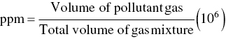
Note that the denominator in Eq. (3.8) is the total volume of gas and not just the volume of air. The results are similar at low concentrations but are not exactly the same, as shown in the following example problem.
For engineering purposes, the results in Example 3.4 might well be considered identical, but at concentrations ranging upward from a few percent (2.0% = 20 000 ppm), a misunderstanding of the definition will result in significantly wrong answers.
Recall that the two common measures of concentration in air pollution work are ppm and μg/m3. By using the ideal gas law, it is relatively straightforward to convert ppm to μg/m3. However, it is necessary to specify a temperature and a pressure because a gas may occupy different volumes depending on these parameters in air pollution work; the reference conditions are usually chosen as 25 °C and 1.0 atm.
Solving the ideal gas law first for the volume of the pollutant and then for the volume of the total gas and relating the two volumes, we obtain the volume fraction as
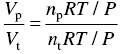
where the subscripts p and t indicate pollutant gas and total gas, respectively. Recognizing that np is merely Mp/M·Wp, Eq. (3.9) can be rearranged as
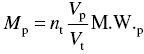
or, substituting for nt,
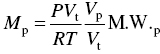
The mass concentration of pollutant is
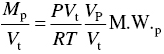
With P = 1.0 atm, T = 298 K (25 °C), and R = 0.082 06 l‐atm/gmol‐K, then P/RT has a value of 0.0409 gmol/l, which is the reciprocal of the molar volume of an ideal gas at the stated conditions.
The mass concentration given by Eq. (3.12) has units of g/l which are not the most convenient for reporting pollutant concentrations in air. To obtain the more common units of μg/m3, the left side of Eq. (3.12) must be multiplied by a factor of 109 (the product of 103 l/m3 and 106 μg/g)
Furthermore, to substitute ppm into Eq. (3.12) for the volume fraction, it is necessary to divide by a factor of (10)6 because ppm is numerically one million times greater than the volume fraction. The net effect is to multiply the right side of Eq. (3.12) by a factor of 1000. Thus, in the form we desire, Eq. (3.12) becomes
Keep in mind that in the air pollution work, it is typical to define standard temperature as 25 °C (298 K). Where the volume per mole of an ideal gas has the value 22.4 l/mol at T = 0 °C (273 K) and P = 1 atm.
So the final version is
where Cmass = mass concentration (μg/m3) and Cppm = volume concentration (ppm).
3.11 Other Applications of the Ideal Gas Law
As mentioned in Section 3.10, the ideal gas law is extremely important to air pollution engineers. Compliance with federal and state laws requires not only proper environmental engineering design and operation of pollution abatement equipment but also careful analysis and accurate measurements of specified pollutants and environmental quality parameters. In the design process and in other types of calculations, engineers who have complete understanding of the ideal gas law will achieve greater accuracy with a smaller expenditure of their time. In this section, through the USE of example problems, we will review various uses of the ideal gas law.
Emission sampling is another important area for which a good understanding of the ideal gas law and the equipment used to measure gas flow is important. Many poorly performing systems are results not of bad design practice but of poor sampling techniques.
Some important considerations in gas sampling are equipment calibration, leaks, sample handling (condensation, adsorption), process operation fluctuations, and representative sampling of the process stream. We will address some of these considerations in the following examples.
When Eq. (3.5) was first presented, one widely used value of R was given for a specific set of units. There are many numerical values of R depending on the units chosen for P, T, V, and n. Table C.3 provides a list of several possible values of R, and the derivation of one such value is illustrated in Example 3.8.
In this example problem, more significant figures were used than are typically used in engineering calculations. Engineers often are satisfied with only three‐ or four‐digit significance. Indeed, the data derived from field measurements are often accurate only to two significant figures. In an age of pocket calculators and personal computers, when it has become routine to obtain numerical answers to eight decimal places, it is important to understand the significance of the numbers we work with. When high accuracy and precision are needed and justified, then many significant figures should be used. However, in many design problems the equations are modified by empirical relationships and must be considered to be approximate.
The weighted‐average molecular weight of a mixture of ideal gases is calculated using mole fractions or volume fractions (not mass fractions) as the weighting factors. This is demonstrated in the following example problem.
3.12 Gas Flow Measurement
A fixed number of moles of gas at a certain temperature and pressure occupies a certain volume. If the pressure and temperature of this fixed number of moles of gas are changed, then the new volume can be easily calculated. Equation (3.5) can be written as follows:
Since n is constant in this case, applying Eq. (3.14) to the two sets of conditions yields
or
Equation (3.16) can be applied to a static system or to a flow system as long as the number of moles under consideration remains constant.
In the preceding example problem, if a concentration of, say, 500 ppm of NO2 were measured in the gases exiting the flow meter, then we could state that the concentration in the stack was also 500 ppm. The reason for this is that ppm is a measure of relative concentration and as the total volume of the gas sample changes, so does the volume of NO2. The relative volume of NO2 (relative to the total) does not change. However, if some moles of a material that is gaseous in the stack are removed from the gas sample stream (such as water that is condensed in the impingers), we must account for the change in relative gas concentrations at the two places (upstream versus downstream of the impingers). This is shown in the following example problem.
3.13 Flow at Standard Temperature and Pressure
Flow at standard temperature and pressure (STP) can be determined provided actual temperature and pressure of the flow are known. Using EPA's standard conditions 20 °C (68 °F), flow at STP becomes:
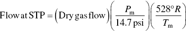
where Pm is the measured pressure in psi and Tm is the measured temperature in °R (°R = 460 + °F).
3.14 Gas Flowrate Conversion from SCFM to ACFM
3.15 Corrections for Percent O2
Corrections for percent O2 are often needed for referencing combustion source emissions. For boilers, comparisons are made at 3% oxygen, consistent with the near stoichiometric conditions in boiler combustors. For combustion turbines, comparisons are made at 15% oxygen, consistent with the high excess air flow in a combustion turbine. To correct for concentrations at other oxygen levels, the following equation is used (Eq. 3.16):

where m% O2 is the nonstandard oxygen concentration. To calculate the concentration at 15% O2, substitute 15.0 for 3.0 in Eq. (3.18).
3.16 Boiler Flue Gas Concentrations Are Usually Corrected to 3% Oxygen
3.17 Air‐to‐Fuel Ratio and Stoichiometric Ratio
In combustion of a hydrocarbon fuel, it is important to accurately calculate the mass of air‐to‐fuel ratio (AFR). Then, the stoichiometric ratio (SR) can be defined as the actual AFR divided by the stoichiometric AFR, as illustrated by the following equation:
The complete combustion of hydrocarbons produces CO2, the desirable aspect of rapid combustion, although CO2 is also an agent of global warming. The following equation shows the reaction:
From a practical standpoint, discounting the disastrous effect of CO2 on global warming, Eq. (3.7) is the desirable reaction. This reaction liberates all the heats of reaction of the hydrocarbon.
The study of combustion frequently uses the terms percent excess air, SR, and equivalence ratio. Percent excess air is the difference between the actual mass of air used and the theoretical divided by the theoretical times 100. The SR is the ratio of the theoretical fuel/air mass ratio to the actual fuel/air mass ratio. The equivalence ratio is the reciprocal of the SR. Air is 21% O2 and 79% N2.
3.18 Material Balances and Energy Balances
Material balances, also called mass balances and energy balances, are applications of conservation of mass and energy to the analysis of physical systems. Process and equipment selections and sizing require a complete knowledge of all material and energy flow to and from each unit. By accounting for material and/or energy entering and leaving a system, mass and/or flows can be identified which might have been unknown or difficult to measure without this technique. The exact conservation law used in the analysis of the system depends on the context of the problem, but all revolve around mass and energy conservation, i.e. that matter or energy cannot be destroyed or created spontaneously (Haugen et al. 1954; Himmelblau 1998).
The general form quoted for a mass balance is the mass that enters a system must, by conservation of mass, either leave the system or accumulate within the system.
For a steady‐state operation, all operating parameters are time independent, and Eq. (3.21) becomes
Therefore, mass balances are used widely in engineering and environmental analyses. For example, mass balance theory is used to design chemical reactors, to analyze alternative processes to produce chemicals, as well as to model pollution dispersion and other processes of physical systems. In majority of cases, Eq. (3.21) describes material and energy balance around pollution control equipment that is designed for steady‐state operation. Some exceptions to this generalization are encountered in the design of incinerators, direct‐fired dryers, and adsorbers owing to the heat generation and/or pollutant accumulation within the units.
In environmental monitoring, the term budget calculations is used to describe mass balance equations where they are used to evaluate the monitoring data (comparing input and output, etc.) In biology the dynamic energy budget theory for metabolic organization makes explicit use of mass and energy balance.
The following steps are helpful in performing materials and energy balance calculations:
- Draw a sketch of the process
- Identify and label all entering and exiting streams
- Label all pertinent data on the sketch
- Draw a dashed envelope around that portion of the process involved in the balance
- Select a suitable basis for the calculation.
3.19 Wastes in the United States
As a nation, Americans officially generate more waste than any other nation in the world, with more than 12 billion T of industrial waste are generated annually in the United States. And the United States's “waste stream” comes from manufacturing, retailing, and commercial trade in the US economy. This is equivalent to more than 40 T of waste for every man, woman, and child in the country. The sheer magnitude of these numbers is cause for concern and drives us to identify the characteristics of the wastes, the industrial operations that are generating the waste, and the manner in which the waste are being managed.
Waste may be defined differently in legislation and regulations of the federal government or individual states. Title 40 of the Code of Federal Regulations dealing with protection of the environment contains at least four different definitions of waste at sections 60.111b, 61.341, 191.12 and 704.83. Definitions may apply broadly to solid, liquid, and gaseous forms or may be specific to one or a subset identified by a threshold characteristic such as toxicity or radioactivity. Discarding, discharge, or disposal (as opposed to sales) is often a requirement for identification as waste, although stored or recycled material may be included within some definitions, and those definitions may reduce recycling options (King 1995).
3.19.1 Industrial Wastes Management Approach
In this section, we will focus on the best available industrial processes, techniques, and technologies that treat wastestreams, including sold and hazardous wastes, as well as innovative and emerging processes that have better potential for achieving the highest standards in pollution prevention at the plant level, leading to zero effect and zero defect (ZED). To move toward ZED via “process pollution prevention” (P3), industries must use processes that deploy materials and energy efficiently enough to neutralize contaminants in the waste stream. The ultimate goal is to remove pollutants from the waste streams and convert them into products or feeds for other processes. Logically then, P3 refers to industrial processes by which materials and energy are efficiently utilized to achieve the end product(s) while reducing or eliminating the creation of pollutants or waste at the source.
Industrial waste is the waste produced by industrial activity which includes any material that is rendered useless during a manufacturing process such as that of factories, industries, mills, mining operations, and thermal and nuclear power plant. Some examples of industrial wastes are chemical solvents, pigments, sludge, metals, ash, paints, sandpaper, paper products, industrial by‐products, metals, and radioactive wastes.
Toxic waste, chemical waste, industrial solid waste, and municipal solid waste (i.e. primary and secondary sludge from POTWs) are designations of industrial wastes. Wastewater treatment plants can treat some industrial wastes, i.e. those consisting of conventional pollutants such as BOD, COD, and TSS). Industrial wastes containing toxic pollutants require specialized treatment systems.
3.19.2 Waste as Pollution
A waste is defined as an unwanted by‐product or damaged, defective, or superfluous material of a manufacturing process. Most often, in its current state, it has or is perceived to have no value. It may or may not be harmful or toxic if released to the environment. Pollution is any release of waste to environment (i.e. any routine or accidental emission, effluent, spill, discharge or disposal to the air, land, or water) that contaminates or degrades the environment.
In 2010, Americans generated about 270 million T of municipal solid waste (MSW), an increase of 16% over 2000 and 53% over 1980 (USEPA 2012). Thus, management of MSW continues to be an important challenge facing the United States and other highly industrialized nations in the twenty‐first century. Solid waste management is critical in the developed world, and developing world as well, where age‐old traditions of wasting nothing (recycle and reuse) are often followed without regard to the significance and implications of the ZED concept.
3.19.3 Why Recycle?
Each ton of solid waste diverted from disposal, whether reused, recycled, converted in a waste‐to‐energy (WtE) program or composted is one less ton of solid waste requiring disposal. To see the value of reusing, recycling, and composting solid waste, one need to simply consider the amount of disposal space required to accept that material. By implementing environmentally benign waste management strategies (as well as resource‐management strategies), a population can reduce its dependence on incinerators and landfills. And when recycled materials are substituted for virgin plastics, metal ores, minerals, glass, paper and trees, there is less pressure to expand the chemical, mining, and forestry industries. Supplying industry with recycled materials is preferable to extracting virgin resources from mines and forests not only because it conserves scarce natural resources but because it reduces dangerous air and water pollutants, such as greenhouse‐gas emissions and saves energy.
Saving energy is an important environmental benefit of recycling because generating energy usually requires fossil‐fuel consumption and results in emissions that pollute the air and water. The energy required to manufacture paper, plastics, glass, and metal from recycled materials is generally less than the energy required to produce them from virgin materials. Additionally, the collection, processing, and transportation of recycled materials typically uses less energy than the extraction, refinement, transportation, and processing steps to which virgin materials must be subjected before industry can use them.
As is well known, a great amount of energy used in industrial processes and in transportation comes from the burning of fossil fuels. Recycling helps stem the dangers of global climate change by reducing the amount of energy used by industry, thus reducing greenhouse‐gas emissions as well.
3.19.4 Chemical Waste
Chemical waste is a waste that is made from harmful chemicals (mostly produced by large factories). Chemical waste may fall under regulations such as COSHH in the United Kingdom, or the CWA and Resource Conservation and Recovery Act (RCRA) in the United States. In the United States, the EPA and the Occupational Safety and Health Administration (OSHA), as well as state and local regulations also regulate chemical use and disposal (Hallam 2010). Chemical waste may or may not be classed as hazardous waste. A chemical hazardous waste is a solid, liquid, or gaseous material that displays either a “hazardous characteristic” or is specifically “listed” by name as a hazardous waste (for HAPs, see Appendix C.1). There are four characteristics chemical wastes may have to be considered as hazardous. These are ignitability, corrosivity, reactivity, and toxicity. This type of hazardous waste must be categorized as to its identity, constituents, and hazards so that it may be safely handled and managed (University of Pennsylvania 2016). Chemical waste is a broad term and encompasses many types of materials. Consult the Material Safety Data Sheet, Product Data Sheet, or Label for a list of constituents. These sources should state whether this chemical waste is a waste that needs special disposal (University of Pennsylvania 2016).
3.19.5 Electronic Waste
Electronic waste in the United States have become an ever‐growing problem in the United States. Each year, over 3.2 million T of electronic waste is put in US landfills. A large portion of this electronic waste is computers, monitors, and televisions. Over 100 million computers, monitors, and televisions are disposed of yearly in the United States (Weidenhamer and Clement 2007). Although there is an enormous amount of electronic waste in the United States, the EPA found that in 2009 approximately only about 25% of all electronic waste is recycled in the United States. About 70% of metals that are found in the United States landfills come from electronic devices. The disposal of all this electronic waste has a detrimental effect on the environment, as well as the global economy.
Electronic waste has become serious issue for the environmental stability in the United States. Over the years, the government has become increasingly more involved in this issue. As described in the USEPA office of RCRA report of 2009, after the electronic products are purchased and used, they are separated into two groups. One group of electronics is collected for recycling, while the other is disposal. After this, the products that are at disposal mainly are put into landfills, and the rest of the electronics that were collected for recycling are either refurbished, reused, or used for material (Stephenson 2008). Hans Tammemagi, the author of The Waste Crisis, talks about the detrimental effect the waste has on the environment. Nearly 20% of all waste in the United States is being incinerated, while the rest of it is being put into landfills (Tammemagi 1999). That leaves almost 80% of the waste consumed in the United States being placed into landfills. Out of this 80% of the waste, the majority of this waste is primarily electronic.
3.20 Hazardous Waste
Hazardous waste is waste that poses substantial or potential threats to public health or the environment (see Table C2 (“a”, “b”, “c”, “d”)). In the United States, the treatment, storage, and disposal of hazardous waste are regulated under the RCRA. Hazardous wastes are defined under RCRA in the Title 40 CFR 261 where they are divided into two major categories: characteristic wastes and listed wastes.
- Characteristic hazardous wastes are materials that are known or tested to exhibit one or more of the following four hazardous traits:
- ignitability
- reactivity
- corrosivity
- toxicity
- Listed hazardous wastes are materials specifically listed by regulatory authorities as hazardous wastes which are from nonspecific sources, specific sources, or discarded chemical products (Shibamoto et al. 2007).
The requirements of RCRA apply to all the companies that generate hazardous waste as well as those companies that store or dispose hazardous waste in the United States. Many types of businesses generate hazardous waste. Dry cleaners, automobile repair shops, hospitals, exterminators, and photo‐processing centers may all generate hazardous waste. Some hazardous waste generators are larger companies such as chemical manufacturers, electroplating companies, and oil refineries.
These wastes may be found in different physical states such as gaseous, liquids, or solids. A hazardous waste is a special type of waste because it cannot be disposed of by common means like other by‐products of our everyday lives. Depending on the physical state of the waste, treatment and solidification processes might be required.
Worldwide, the United Nations Environmental Program estimated that more than 400 million T of hazardous wastes are produced universally each year, mostly by industrialized countries. About 1% of this is shipped across international boundaries, with the majority of the transfers occurring between countries in the Organization for the Economic Cooperation and Development. One of the reasons for industrialized countries to ship the hazardous waste to industrializing countries for disposal is the rising cost of disposing of hazardous waste in the home country (Orloff and Henry 2003).
3.20.1 Hazardous Wastes in the United States of America
A US facility that treats, stores, or disposes of hazardous waste must obtain a permit for doing so under the RCRA. Generators and transporters of hazardous waste must meet specific requirements for handling, managing, and tracking waste. Through the RCRA, Congress directed the EPA to create regulations to manage hazardous waste. Under this mandate, the EPA developed strict requirements for all aspects of hazardous waste management including the treatment, storage, and disposal of hazardous waste. In addition to these federal requirements, states may develop more stringent requirements that are broader in scope than the federal regulations. Furthermore, RCRA allows states to develop regulatory programs that are at least as stringent as RCRA and, after review by EPA, the states may take over responsibility for the implementation of the requirements under RCRA. Most states take advantage of this authority, implementing their own hazardous waste programs that are at least as stringent, and in some cases are more stringent than the federal program.
3.20.2 Hazardous Waste Mapping Systems
The US government provides several tools for mapping hazardous wastes to particular locations. These tools also allow the user to view additional information.
- TOXMAP is a Geographic Information System from the Division of Specialized Information Services of the United States National Library of Medicine (NLM) that uses maps of the United States to help users visually explore data from the USEPA's Toxics Release Inventory and Superfund Basic Research Programs. This is a resource funded by the US federal government. TOXMAP's chemical and environmental health information is taken from NLM's Toxicology Data Network and PubMed, and from other authoritative sources.
- The USEPA “Where You Live” (Chaudhary and Rachana 2006) allows users to select a region from a map to find information about Superfund sites in that region.
3.20.3 Universal Wastes
Universal wastes are a special category of hazardous wastes that (in the United States):
- generally pose a lower threat relative to other hazardous wastes that are ubiquitous and produced in very large quantities by a large number of generators.
Some of the most common “universal wastes” are fluorescent light bulbs, some specialty batteries (e.g. lithium‐ or lead‐containing batteries), cathode ray tubes, and mercury‐containing devices.
Universal wastes are subject to somewhat less stringent regulatory requirements. Small quantity generators of universal wastes may be classified as “conditionally exempt small quantity generators” which release them from some of the regulatory requirements for the handling and storage of hazardous wastes. Universal wastes must still be disposed of properly at a regional or county landfill facility.
3.20.4 Final Disposal of Hazardous Waste
Historically, some hazardous wastes were disposed of in regular landfills. This resulted in unfavorable amounts of hazardous materials seeping into the ground. These chemicals eventually entered to natural hydrologic systems. Many landfills now require countermeasures against groundwater contamination. For example, a barrier has to be installed along the foundation of the landfill to contain the hazardous substances that may remain in the disposed waste. Currently, hazardous wastes must often be stabilized and solidified in order to enter a landfill and must undergo different treatments in order to stabilize and dispose them. Most flammable materials can be recycled into industrial fuel. Some materials with hazardous constituents can be recycled, such as lead acid batteries.
3.20.5 Recycling
Some hazardous wastes can be recycled into new products. Examples may include lead‐acid batteries or electronic circuit boards. When heavy metals in these types of ashes go through the proper treatment, they could bind to other pollutants and convert them into easier‐to‐dispose solids, or they could be used as pavement filling. Such treatments reduce the level of threat of harmful chemicals, like fly and bottom, while also recycling the safe product.
3.20.6 Portland Cement
Another commonly used treatment is cement‐based solidification and stabilization. Cement is used because it can treat a range of hazardous wastes by improving physical characteristics and decreasing the toxicity and transmission of contaminants. The cement produced is categorized into five different divisions, depending on its strength and components. This process of converting sludge into cement might include the addition of pH adjustment agents, phosphates, or sulfur reagents to reduce the settling or curing time, increase the compressive strength, or reduce the leach ability of contaminants.
3.21 Incineration, Destruction, and WtE
Hazardous waste may be “destroyed.” For example, by incinerating it at a high temperature, flammable wastes can sometimes be burned as energy sources. For example, many cement kilns burn hazardous wastes like used oils or solvents. Today, incineration treatments not only reduce the amount of hazardous waste but also generate energy from the gases released in the process. It is known that this particular waste treatment releases toxic gases produced by the combustion of by‐product or other materials which can affect the environment. However, current technology has developed more efficient incinerator units that control these emissions to a point where this treatment is considered a more beneficial option. There are different types of incinerators which vary depending on the characteristics of the waste. Starved air incineration is another method used to treat hazardous wastes. Just like in common incineration, burning occurs, however, controlling the amount of oxygen allowed proves to be significant to reduce the amount of harmful by‐products produced. Starved air incineration is an improvement of the traditional incinerators in terms of air pollution. Through using this technology, it is possible to control the combustion rate of the waste and therefore reduce the air pollutants produced in the process (see a Case Study on WtE in Sections 7.13.1.1 and 7.13.3).
3.22 Hazardous Waste Landfill (Sequestering, Isolation, etc.)
Hazardous waste may be sequestered in an hazardous waste landfill or permanent disposal facility. “In terms of hazardous waste, a landfill is defined as a disposal facility or part of a facility where hazardous waste is placed or on land and which is not a pile, a land treatment facility, a surface impoundment, an underground injection well, a salt dome formation, a salt bed formation, an underground mine, a cave, or a corrective action management unit” (Title 40 CFR 260.10).
3.22.1 Pyrolysis
Some hazardous waste types may be eliminated using pyrolysis in an ultrahigh temperature electrical arc, in inert conditions to avoid combustion. This treatment method may be preferable to high‐temperature incineration in some circumstances such as in the destruction of concentrated organic waste types, including PCBs, pesticides, and other persistent organic pollutants (RCRA, USEPA, Title 40 CFR 261).
3.23 Radioactive Waste
Radioactive waste is waste that contains radioactive material. Radioactive waste is usually a by‐product of nuclear power generation and other applications of nuclear fission or nuclear technology such as research and medicine. Radioactive waste is hazardous to all forms of life and the environment, and it is regulated by government agencies in order to protect human health and the environment.
Radioactivity naturally decays over time; therefore, radioactive waste has to be isolated and confined in appropriate disposal facilities for a sufficient period until it no longer poses a threat. The time radioactive waste must be stored for depends on the type of waste and radioactive isotopes. Current approaches to managing radioactive waste have been segregation and storage for short‐lived waste, near‐surface disposal for low and some intermediate level waste, and deep burial or partitioning/transmutation for the high‐level waste.
A summary of the amounts of radioactive waste and management approaches for most developed countries are presented and reviewed periodically as part of the International Atomic Energy Agency (IAEA) Joint Convention on the Safety of Spent Fuel Management and on the Safety of Radioactive Waste Management (IAEA 2007).
3.23.1 Sources
Radioactive waste comes from a number of sources. In countries with nuclear power plants, nuclear armament or nuclear fuel treatment plants, the majority of waste originates from the nuclear fuel cycle and nuclear weapons reprocessing. Other sources include medical and industrial wastes as well as naturally occurring radioactive materials (NORM) that can be concentrated as a result of the processing or consumption of coal, oil, and gas and some minerals as discussed below.
3.23.2 Nuclear Fuel Cycle
3.23.2.1 Front End
Waste from the front end of the nuclear fuel cycle is usually alpha‐emitting waste from the extraction of uranium. It often contains radium and its decay products.
Uranium dioxide (UO2) concentrate from mining is a thousand or so times as radioactive as the granite used in buildings. It is refined from yellowcake (U3O8), then converted to uranium hexafluoride gas (UF6). As a gas, it undergoes enrichment to increase the U‐235 content from 0.7% to about 4.4% low enriched uranium (LEU). It is then turned into a hard ceramic oxide (UO2) for assembly as reactor fuel elements (Cochran 1999).
The main by‐product of enrichment is depleted uranium (DU), principally the U‐238 isotope, with a U‐235 content of approximately 0.3%. It is stored either as UF6 or as U3O8. Some is used in applications where its extremely high density makes it valuable such as antitank shells, and on at least one occasion even a sailboat keel (IHS Jane's 360). It is also used with plutonium for making mixed oxide fuel and to dilute, or downblend, highly enriched uranium from weapons stockpiles which is now being redirected to become reactor fuel.
3.23.2.2 Back End
The back‐end of the nuclear fuel cycle, mostly spent fuel rods, contains fission products that emit beta and gamma radiation, and actinides that emit alpha particles, such as uranium‐234 (half‐life 245 000 years), neptunium‐237 (2.144 million years), plutonium‐238 (87.7 years), and americium‐241 (432 years), and even sometimes some neutron emitters such as californium (half‐life of 898 years for Cf‐251). These isotopes are formed in nuclear reactors.
It is important to distinguish the processing of uranium to make fuel from the reprocessing of used fuel. Used fuel contains the highly radioactive products of fission (see Section 3.25.2). Many of these are neutron absorbers, called neutron poisons in this context. These eventually build up to a level where they absorb so many neutrons that the chain reaction stops, even with the control rods completely removed. At that point, the fuel has to be replaced in the reactor with fresh fuel, even though there is still a substantial quantity of uranium‐235 and plutonium present. In the United States, this used fuel is usually “stored,” while in other countries such as Russia, the United Kingdom, France, Japan, and India, the fuel is reprocessed to remove the fission products, and the fuel can then be reused, thus cutting costs, reducing health risks, saving time, and in general being far safer (Regulation of TENORM 2012). The fission products removed from the fuel are a concentrated form of high‐level waste as are the chemicals used in the process. While these countries reprocess the fuel carrying out single plutonium cycles, India is the only country known to be planning multiple plutonium recycling schemes.
3.23.2.3 Nuclear Industry
Industrial source waste can contain alpha, beta, neutron, or gamma emitters. Gamma emitters are used in radiography, while neutron emitting sources are used in a range of applications, such as oil well logging (Nuclear Logging 2009).
Annual release of uranium and thorium radioisotopes from coal combustion, predicted by ORNL, cumulatively amount to 2.9 million T over the 1937–2040 period, from the combustion of an estimated 637 billion T of coal worldwide (Gabbard 1993).
Substances containing natural radioactivity are known as NORM. After human processing that exposes or concentrates this natural radioactivity (such as mining bringing coal to the surface or burning it to produce concentrated ash), it becomes technologically enhanced NORM (TENORM) (USEPA, June 6 2006c). A lot of this waste is alpha particle‐emitting matter from the decay chains of uranium and thorium. The main source of radiation in the human body is potassium‐40 (°K), typically 17 mg in the body at a time and 0.4 mg/day intake (Radio activity in nature, Idaho State University). Most rocks, due to their components, have a low level of radioactivity. Usually ranging from 1 to 13 mSv annually depending on location, average radiation exposure from natural radioisotopes is 2.0 mSv/person a year worldwide (UNSCEAR 2008). This makes up the majority of typical total dosage (with mean annual exposure from other sources amounting to 0.6 mSv from medical tests averaged over the whole populace, 0.4 mSv from cosmic rays, 0.005 mSv from the legacy of past atmospheric nuclear testing, 0.005 mSv occupational exposure, 0.002 mSv from the Chernobyl disaster, and 0.0002 mSv from the nuclear fuel cycle) (UNSCEAR 2008).
TENORM is not regulated as restrictively as nuclear reactor waste, though there are no significant differences in the radiological risks of these materials (Regulation of TENORM, Aug 1 2012).
3.24 Coal
Coal contains a small amount of radioactive uranium, barium, thorium, and potassium but, in the case of pure coal, this is significantly less than the average concentration of those elements in the Earth's crust. The surrounding strata, if shale or mudstone, often contain slightly more than average and this may also be reflected in the ash content of “dirty” coals (Gabbard 1993; Cosmic Origin of Uranium 2006). The more active ash minerals become concentrated in the fly ash precisely because they do not burn well (Gabbard 1993). The radioactivity of fly ash is about the same as black shale and is less than phosphate rocks, but it is more of a concern because a small amount of the fly ash ends up in the atmosphere where it can be inhaled (U.S. Geological Survey 1997). According to U.S. NCRP reports, population exposure is from 1000‐MWe power plants amounts to 490 person‐rem/year for coal power plants, and thus is 100 times as great as nuclear power plants (4.8 person‐rem/year). (The exposure from the complete nuclear fuel cycle from mining to waste disposal is 136 person‐rem/year; the corresponding value for coal use from mining to waste disposal is “probably unknown”) (Gabbard 1993).
3.24.1 Oil and Gas
Residues from the oil and gas industry often contain radium and its decay products. The sulfate scale from an oil well can be very radium rich, while the water, oil, and gas from a well often contain radon. The radon decays to form solid radioisotopes which form coatings on the inside of pipe‐work. In an oil‐processing plant, the area of the plant where propane is processed is often one of the more contaminated areas of the plant as radon has a similar boiling point to propane.
3.25 Low‐Level Waste
Low‐level waste (LLW) is generated from hospitals and industry, as well as the nuclear fuel cycle. LLWs include paper, rags, tools, clothing, filters, and other materials which contain small amounts of mostly short‐lived radioactivity. Materials that originate from any region of an Active Area are commonly designated as LLW as a precautionary measure even if there is only a remote possibility of being contaminated with radioactive materials. Such LLW typically exhibits no higher radioactivity than one would expect from the same material disposed of in a non‐active area, such as a normal office block.
Some high‐activity LLW requires shielding during handling and transport, but most LLW is suitable for shallow land burial. To reduce its volume, it is often compacted or incinerated before disposal. LLW is divided into four classes: class A, class B, class C, and greater than class C.
3.25.1 Intermediate‐Level Waste
Intermediate‐level waste (ILW) contains higher amounts of radioactivity and in general require shielding, but not cooling (USNRC, April 3 2017). ILWs includes resins, chemical sludge, and metal nuclear fuel cladding, as well as contaminated materials from reactor decommissioning. It may be solidified in concrete or bitumen for disposal. As a general rule, short‐lived waste (mainly nonfuel materials from reactors) is buried in shallow repositories, while LLW (from fuel and fuel reprocessing) is deposited in geological repository. US regulations do not define this category of waste; the term is used in Europe and elsewhere.
3.25.2 High‐Level Waste
High‐level waste (HLW) is produced by nuclear reactors. The exact definition of HLW differs internationally. After a nuclear fuel rod serves one fuel cycle and is removed from the core, it is considered HLW (Janicki 2013). Fuel rods contain fission products and transuranic elements generated in the reactor core. Spent fuel is highly radioactive and often hot. HLW accounts for over 95% of the total radioactivity produced in the process of nuclear electricity generation. The amount of HLW worldwide is currently increasing by about 12 000 MT every year, which is the equivalent to about 100 double‐decker buses or a two‐story structure with a footprint the size of a basketball court (Rogner 2010). A 1000‐MW nuclear power plant produces about 27 T of spent nuclear fuel (unreprocessed) every year (Myths and Realities of Radioactive Waste, Feb. 2017). In 2010, there was very roughly estimated to be stored some 250 000 T of nuclear HLW (World Nuclear Association, July 2015) that does not include amounts that have escaped into the environment from accidents or tests. Japan estimated to hold 17 000 T of HLW in storage in 2015 (Geere 2010). HLWs have been shipped to other countries to be stored or reprocessed, and in some cases, shipped back as active fuel.
The ongoing controversy over high‐level radioactive waste disposal is a major constraint on the nuclear power's global expansion (Humber 2015). Most scientists agree (Findlay 2010) that the main proposed long‐term solution is deep geological burial, either in a mine or a deep borehole. However, almost six decades after commercial nuclear energy began, no government has succeeded in opening such a repository for civilian high‐level nuclear waste (Humber 2015), although Finland is in the advanced stage of the construction of such facility, the Onkalo spent nuclear fuel repository. Reprocessing or recycling spent nuclear fuel options already available or under active development still generate waste and so are not a total solution, but it can reduce the sheer quantity of waste, and there are many such active programs worldwide. Deep geological burial remains the only responsible way to deal with high‐level nuclear waste (World Nuclear Association 2015). The Morris Operation is currently the only de facto high‐level radioactive waste storage site in the United States.
3.25.3 Transuranic Waste
Transuranic waste (TRUW) as defined by US regulations is, without regard to form or origin, waste that is contaminated with alpha‐emitting transuranic radionuclides with half‐lives greater than 20 years and concentrations greater than 100 nCi/g (3.7 MBq/kg), excluding HLW. Elements that have an atomic number greater than uranium are called transuranic (“beyond uranium”). Because of their long half‐lives, TRUW is disposed more cautiously than either low‐ or intermediate‐level waste. In the United States, it arises mainly from weapons production and consists of clothing, tools, rags, residues, debris, and other items contaminated with small amounts of radioactive elements (mainly plutonium).
Under US law, transuranic waste is further categorized into “contact‐handled” (CH) and “remote‐handled” (RH) on the basis of the radiation dose rate measured at the surface of the waste container. CH TRUW has a surface dose rate not greater than 200 mrem/h (2 mSv/h), whereas RH TRUW has a surface dose rate of 200 mrem/h (2 mSv/h) or greater. CH TRUW does not have the very high radioactivity of HLW nor its high heat generation, but RH TRUW can be highly radioactive, with surface dose rates up to 1 000 000 mrem/h (10 000 mSv/h). The United States currently disposes of TRUW generated from military facilities at the Waste Isolation Pilot Plant in a deep salt formation in New Mexico (Biello 2011).
3.26 Nuclear Waste Management
Of particular concern in nuclear waste management are two long‐lived fission products, Tc‐99 (half‐life 220 000 years) and I‐129 (half‐life 15.7 million years), which dominate spent fuel radioactivity after a few thousand years. The most troublesome transuranic elements in spent fuel are Np‐237 (half‐life two million years) and Pu‐239 (half‐life 24 000 years) (Nuclear Decommissioning Authority 2014). Nuclear waste requires sophisticated treatment and management to successfully isolate it from interacting with the biosphere. This usually necessitates treatment, followed by a long‐term management strategy involving storage, disposal, or transformation of the waste into a nontoxic form (Vandenbosch and Vandenbosch 2007). Governments around the world are considering a range of waste management and disposal options, though there has been limited progress toward long‐term waste management solutions (Ojovan and Lee 2014).
In the second half of twentieth century, several methods of disposal of radioactive waste were investigated by nuclear nations (Brown 2004), which are as follows:
- “Long term above ground storage,” not implemented
- “Disposal in outer space” (for instance, inside the Sun), not implemented – as it would be currently too expensive
- “Deep borehole disposal,” not implemented
- “Rock‐melting,” not implemented
- “Disposal at subduction zones,” not implemented
- “Ocean disposal,” done by the USSR, the United Kingdom (World Nuclear Association 2011), Switzerland, the United States, Belgium, France, The Netherlands, Japan, Sweden, Russia, Germany, Italy, and South Korea (1954–1993). This is no longer permitted by international agreements.
- “Sub seabed disposal,” not implemented, not permitted by international agreements
- “Disposal in ice sheets,” rejected in Antarctic Treaty
- “Direct injection,” done by USSR and United States.
In the United States, waste management policy completely broke down with the ending of work on the incomplete Yucca Mountain Repository (The Independent London 1997). At present, there are 70 nuclear power plant sites where spent fuel is stored. A Blue Ribbon Commission was appointed by President Obama to look into future options for this and future waste. A deep geological repository seems to be favored (The Independent London 1997).
3.26.1 Initial Treatment
3.26.1.1 Vitrification
Long‐term storage of radioactive waste requires the stabilization of the waste into a form which will neither react nor degrade for extended periods. It is theorized that one way to do this might be through vitrification (Blue Ribbon Commission 2012). Currently, at Sellafield the HLW (PUREX first cycle raffinate) is mixed with sugar and then calcined. Calcination involves passing the waste through a heated, rotating tube. The purposes of calcination are to evaporate the water from the waste, and denitrate the fission products to assist the stability of the glass produced.
The “calcine” generated is fed continuously into an induction heated furnace with fragmented glass (National Research Council 1996). The resulting glass is a new substance in which the waste products are bonded into the glass matrix when it solidifies. As a melt, this product is poured into stainless steel cylindrical containers (“cylinders”) in a batch process. When cooled, the fluid solidifies (“vitrifies”) into the glass. After being formed, the glass is highly resistant to water (Laboratory‐scale vitrification and leaching of Hanford high‐level waste for the…model verification 2009).
After filling a cylinder, a seal is welded onto the cylinder head. The cylinder is then washed. After being inspected for external contamination, the steel cylinder is stored, usually in an underground repository. In this form, the waste products are expected to be immobilized for thousands of years (Ojovan et al. 2006).
The glass inside a cylinder is usually a black glossy substance. All this work (in the United Kingdom) is done using hot cell systems. Sugar is added to control the ruthenium chemistry and to stop the formation of the volatile RuO4 containing radioactive ruthenium isotopes. In the West, the glass is normally a borosilicate glass (similar to Pyrex), while in the former Soviet Bloc it is normal to use a phosphate glass (Nuclear Energy Agency, Paris 1994). The amount of fission products in the glass must be limited because some (palladium, the other Pt group metals, and tellurium) tend to form metallic phases which separate from the glass. Bulk vitrification uses electrodes to melt soil and wastes, which are then buried underground (Ojovan and Lee 2010). In Germany a vitrification plant is in use; this is treating the waste from a small demonstration reprocessing plant which has since been closed down (Pacific Northwest National Laboratory, PNNL‐15198, July 2005).
3.26.1.2 Ion Exchange
It is common for medium active wastes in the nuclear industry to be treated with ion exchange or other means to concentrate the radioactivity into a small volume. The much less radioactive bulk (after treatment) is often then discharged. For instance, it is possible to use a ferric hydroxide floc to remove radioactive metals from aqueous mixtures (Hensing and Schultz 1995). After the radioisotopes are absorbed onto the ferric hydroxide, the resulting sludge can be placed in a metal drum before being mixed with cement to form a solid waste form (Brünglinghaus, Waste Processing 2013). In order to get better long‐term performance (mechanical stability) from such forms, they may be made from a mixture of fly ash, or blast furnace slag, and Portland cement, instead of normal concrete (made with Portland cement, gravel, and sand).
Problems
- 3.1 The suspended particulate concentration in an aqueous industrial stream has been determined to be 27.6 mg/l. Convert this value to units of μg/l, g/l, lb/ft3, and lb/gal.
- 3.2 A biologically contaminated dairy liquid waste requires disinfection with chlorine prior to discharge into a nearby lake. Given a contact time of 30 minutes, a required chlorine dose for a 99.99% kill of the pathogenic organisms. To carry out the two‐steps oxidation–reduction and complete disinfection, the chlorine doses were kept at 3.0 and 0.5 mg/l, respectively. Calculate how many pounds of chlorine would be required daily to disinfect 100 000 gal/day.
- 3.3 Polymer is supplied to an industrial wastewater pretreatment plant at a concentration of 0.5 lb/gal. The polymer feed pump delivers a flow of 0.1 gpm and the water flow rate to the filter is 3000 gpm. Calculate the dose (in mg/l) of polymer in the water applied to the filter.
- 3.4 Given the waste constituent and concentration shown in the following table, determine the quantity (in kilogram per day) of hydrated lime [Ca(OH)2] required to neutralize the waste. Estimate the TDS after neutralization. Report your answer in milligram per liter (mg/l).
Constituent Concentration (mg/l) Flow (l/min) HCl 100 5 - 3.5 Given the waste constituent and concentration shown in the following table, determine the quantity (in kilogram per day) of sulfuric acid [H2(SO)4] required to neutralize the waste. Estimate the TDS after neutralization. Report your answer in milligram per liter (mg/l).
Constituent Concentration (mg/l) Flow (l/min) NaOH 250 20 - 3.6 The concentration of TCE in an air sample near a hazardous waste landfill is 34 ppm, the ambient air temperature is 31 °C, and the atmospheric pressure is 0.94 atm. What is the TCE concentration in mg/m3?
- 3.7 A sample of air has been collected above an air stripping tower to evaluate its performance and to determine if toxic air emission standards are being violated. The temperature at the time of collection was 18 °C and the atmospheric pressure was 740 mm Hg. The concentrations in the sample were 4.8 mg/m3 of benzene and 1.7 mg/m3 per chloroethylene, and 2.0 mg/m3 of methylene chloride. Calculate the concentrations in ppm using the equation as follows: Cppm = C(RT/PM) × 106, where C is the concentration of the sample in mg/m3, R = 8.21 − 10−5 (m3·atm/mol·K), M is the molecular weight of the gas, and T is the absolute temperature in K.
- 3.8 Liquid alum is usually available at a concentration of 5.4 lb alum/gal. In an industrial wastewater pretreatment application, the alum feed pump delivers 88 ml/min and the flow to the filter is 3000 gpm. Calculate the dose of alum in the water applied to the filter.
- 3.9 An advanced treatment is implemented in industrial wastewater (addition of ferric chloride, FeCl3, and polymer), the BOD is removed in primary treatment by 30–45%. Calculate the inlet BOD load in pounds per day, BOD load, and percent reduction in aeration basin, and the annual chemical cost using the data provided below:
- Flow, Q = 50 MGD
- Influent BOD = 175 mg/l
- FeCl3 = 20 mg/l at 0.012/lb
- Polymer = 0.2 mg/l at $1.70/lb
- 3.10 Determine the time, in hours, required for the concentration of toluene in a wastewater treatment process to be reduced to one‐half of its initial value. Assume the first‐order reaction rate constant for toluene is 0.07/h.
Calculate the time for the toluene to be reduced to 99% of its initial value. Also calculate the time for 99.99% of the toluene to react.
- 3.11 In a pretreatment, industrial wastewater is coagulated with a dosage of 30 mmg/l of aluminum sulfate as alum and an equivalent dosage of lime to neutralize the hydrogen ions produced in the hydrolysis of aluminum. Calculate (a) how many pounds of alum are needed per MG of processed water treated? (b) How many pounds of Al(OH)3 sludge are produced per MG of water treated?
- 3.12 A tannery uses a filter press to dewater its raw sludge. The dewatered sludge contains 120 mg of total chromium/kg of sludge. The filter press has a surface area 150 ft2 with a filtration rate of 10 gal/h·ft2. Assume that it is 100% efficient in separating solids. Estimate the amount of total chromium disposed per year from this plant if the plant operates 16 h/day, and 7 day/week, 50 week/year. The following information is available.
Before dewatering:
After dewatering:

References
- Allen, D. and Rosselot, K. (1997). Pollution Prevention for Chemical Processes. Hoboken, NJ: Wiley.
- Arthur, C. (1997). Ministers admit nuclear waste was dumped in sea. The Independent London (1 July).
- Bateson, T. and Schwartz, J. (2008). Children's response to air pollutants. Journal of Toxicology and Environmental Health 71 (3): 238–243.
- Berglund, R., Wood, D., and Covin, T. (1989). Fugitive Emissions from the Acrolein Production Industry. Paper presented at the Air and Waste Management Association International Specialty Conference: SARA Title III, Section 313, Industry Experience in Estimating Chemical Releases.
- Biello, D. (2011). Presidential Commission Seeks Volunteers to Store U.S. Nuclear Waste. Scientific American (29 July). https://www.scientificamerican.com/article (accessed 21 September 2019).
- Blue Ribbon Commission (2012). America's Nuclear Future: Executive Summary.
- Bond, R.G. and Straub, C.P. (1974). Wastewater, Treatment and Disposal. Cleveland, OH: CRC Press.
- Brown, P. (2004) Shoot it at the Sun. Send it to Earth's Core. What to do with Nuclear Waste? The Guardian (14 April).
- Brünglinghaus, M. (2013). Waste Processing. Euronuclear.org.
- Chambers, A., Wootton, T., Moncrieff, J., and McCready, P. (2008). Direct measurement of fugitive emissions of hydrocarbons from a refinery. Journal of the Air and Waste Management Association 58 (8): 1047–1056.
- Chaudhary, R. and Rachana, M. (2006). Factors affecting hazardous waste solidification/stabilization: A review. Journal of Hazardous Materials B137: 267–276.
- Clearstone Engineering (1994). A National Inventory of Greenhouse Gas (GHG), Criteria Air Contaminant (CAC) and Hydrogen Sulphide (H2S) Emissions by the Upstream Oil and Gas. Industry, Volume 1, Overview of the GHG Emissions Inventory. Canadian Association of Petroleum Producers.
- Cochran, R. (1999). The Nuclear Fuel Cycle: Analysis and Management, 52–57. La Grange Park, IL: American Nuclear Society.
- Cosmic Origins of Uranium (2006). Continuous plutonium recycling in India: improvements in reprocessing technology. uic.com.au.
- Crites, R.W. and Tchobanoglous, G. (1998). Small and Decentralized Wastewater Management Systems. New York, NY: WCB/McGraw‐Hill.
- Eckenfelder, W.W. (2000). Industrial Water Pollution Control, 3e. New York, NY: McGraw‐Hill.
- Findlay, T. (2010). Nuclear Energy to 2030 and Its Implications for Safety, Security and Nonproliferation: Overview. Nuclear Energy Futures Project.
- Gabbard, A. (1993). Coal combustion. ORNL Review 26: 3–4.
- Geere, D. (2010) Where Do You Put 250,000 tonnes of Nuclear Waste? (Wired UK). Wired.co.uk. Global Defence News and Defence Headlines – IHS Jane's 360.
- Hallam, B. (2010). Techniques for efficient hazardous chemicals handling and disposal. Pollution Equipment News (April/May 2010), p. 13.
- Haugen, O.A., Watson, K.M., and Ragatz, R.A. (1954). Chemical Process Principles – Part I: Materials and Energy Balances, 2e. New York: Wiley.
- Hauser, C. (2018). Algal Bloom in Lake Superior Raises Worries on Climate Change and Tourisms. The New York Times (29 August).
- Hensing, I. and Schultz, W. (1995). Economic Comparison of Nuclear Fuel Cycle Options. Cologne: Energiewirtschaftlichen Instituts.
- Himmelblau, D.M. (1998). Basic Principles and Calculations in Chemical Engineering, 2e. Upper Saddle River, NJ: Prentice Hall.
- Humber, Y. (2015). Japan's 17,000 Tons of Nuclear Waste in Search of a Home, Bloomberg. Idaho State University. Radioactivity in Nature.
- Industrial Waste Treatment (IWT) (1999). V1&V2. California State University, USA. http://www.owp.csus.edu/courses/wastewater/industrial‐waste‐treatment‐vol‐i.php (accessed 21 September 2019).
- International Atomic Energy Agency (IAEA). (2007). The Joint Convention.
- Janicki, M. (2013). Iron boxes for ILW transport and storage. Nuclear Engineering International 58 (711): 47–48.
- Kampa, M. and Castanas, E. (2008). Human health effects of air pollution. Environmental Pollution 151 (2): 362–367.
- Karell, M. (2017). Estimating air emission rates. Chemical Engineering Progress 113 (7): 59–65.
- King, J. (1995). The Environmental Dictionary, 745. New York: Wiley.
- Krenkel, P.A. and Novotny, V. (1980). Water Quality Management. Cambridge, MA: Academic Press.
- Chapman, C.C., Buell, J.L., Slate, S.C. et al. (2009). Laboratory‐scale vitrification and leaching of Hanford high‐level waste for the purpose of simulant and glass property models validation.
- Latza, U., Gerdes, S., and Baur, X. (2008). Effects of nitrogen dioxide on human health: systematic review of experimental and epidemiological studies conducted between 2002 and 2006. International Journal of Hygiene and Environmental Health 212 (3): 271–287.
- Metcalf & Eddy (2003). Wastewater Engineering: Treatment and Reuse, 4e. New York: McGraw Hill.
- Moss, B. (2008). Water pollution by agriculture. Philosophical Transactions of the Royal Society B: Biological Sciences 363: 659–666.
- Myths and Realities of Radioactive Waste. (2017).
- National Research Council (1996). Nuclear Wastes: Technologies for Separation and Transmutation. Washington DC: National Academy Press.
- Nuclear Decommissioning Authority (2014). Progress on Approaches to Management of Separated Plutonium. Cumbria: Nuclear Decommissioning Authority.
- Nuclear Logging (2009). https://petrowiki.org/Nuclear_logging (accessed 21 September 2019).
- OECD Nuclear Energy Agency (1994). The Economics of the Nuclear Fuel Cycle. Paris: OECD Nuclear Energy Agency.
- Ojovan, M. and Lee, W. (2010). Glassy wasteforms for nuclear waste immobilization. Metallurgical and Materials Transactions, A 42 (4): 837.
- Ojovan, M. and Lee, W. (2014). An Introduction to Nuclear Waste Immobilization. Amsterdam: Elsevier.
- Ojovan, M., Lee, W., Hand, R., and Ojovan, N. (2006). Corrosion of nuclear waste glasses in non‐saturated conditions: time‐temperature behavior.
- Orloff, K. and Henry, F. (2003). An international perspective on hazardous waste practices. International Journal of Hygiene and Environmental Health 206 (4–5): 291–302.
- Pacific Northwest National Laboratory (2005). Waste Form Release Calculations for the 2005 Integrated Disposal Facility Performance Assessment, PNNL‐15198. Richland: Pacific Northwest National Laboratory.
- Pink, D.H. (2006). Investing in Tomorrow's Liquid Gold, Yahoo, Archived from the Original on 23 April 2006.
- Regulation of TENORM (2012). Recycling spent nuclear fuel: the Ultimate Solution for the US. Archived from the original on 28 November 2012, “Regulation of TENORM”. Tenorm.com.
- Rogner, H. (2010). Nuclear power and stable development. Journal of International Affairs 64: 149.
- Rouessac, F. and Rouessac, A. (2007). Chemical Analysis: Modern Instrumentation Methods and Techniques, 2e. Hoboken, NJ: Wiley.
- Salvi, S. (2007). Health effects of ambient air pollution in children. Pediatric Respiratory Reviews 8 (4): 275–280.
- Shibamoto, T., Yasuhara, A., and Katami, T. (2007). Dioxin formation from waste incineration. Reviews of Environmental Contamination and Toxicology 190: 1–41.
- Stephenson, J. (2008). Electronic Waste: EPA Needs to Better Control Harmful U. S. Exports Through Stronger Enforcement and More Comprehensive Regulations. DIANE Publishing. Survey & Identification of NORM Contaminated Equipment. enprotec‐inc.com.
- Tammemagi, H.Y. (1999). The Waste Crisis. Oxford University Press.
- Title 40 of the Code of Federal Regulations (CFR) (2018).
- USEPA (1975). Technical Support Document: EPA Regulations for Preventing the Significant Deterioration of Air Quality. Research Triangle Park, NC: Office of Air Quality Planning and Standards, Publication EPA‐450/2‐75‐001.
- US Geological Survey (1997). Radioactive Elements in Coal and Fly Ash: Abundance, Forms, and Environmental Significance, Fact Sheet FS‐163‐1997. Reston, VA: U.S. Department of the Interior, U.S. Geological Survey.
- United Nations Scientific Committee on the Effects of Atomic Radiation (2008). Sources and Effects of Ionizing Radiation. UNSCEAR.
- United States Code, Clean Water Act, Section 402(p) 33 U.S.C. §1342(p) (1999).
- United States Code, Clean Water Act, Section 502(14) 33 U.S.C. §1362(14) (1999).
- University of Pennsylvania (2016). Laboratory Chemical Waste Management Guidelines. Environmental Health and Radiation Safety, University of Pennsylvania.
- USEPA (1985a). AP‐42: Compilation of Air Pollutant Emission Factors, Volume I: Stationary Point and Area Sources, 4e, with Supplements A‐D. Research Triangle Park, NC: Office of Air Quality Planning and Standards, Publication AP‐42, 1985.
- USEPA (1985b). A Model for Evaluation of Refinery and Synfuels VOC Emission Data, Volume I. Research Triangle Park, NC: Office of Air Quality Planning and Standards Publication EPA‐600/7‐85‐022a, 1985.
- USEPA (1988). Protocols For Generating Unit‐Specific Emission Estimates For Equipment Leaks of VOC and VHAP. Research Triangle Park, NC: Office of Air Quality Planning and Standards, Publication EPA‐450/3‐88‐010, 1988.
- USEPA (1990). The Clean Air Act Amendments of 1990 Summary Materials. Washington, DC: USEPA, Office of Air and Radiation.
- USEPA (1993). Protocols for Equipment Leak Emission Estimates. Research Triangle Park, NC: Office of Air Quality Planning and Standards, Publication, available through NTIS as PB 229219, June 1993.
- USEPA (1995). Protocols for Equipment Leak Emission Estimates. Research Triangle Park, NC: Office of Air Quality Planning and Standards, Publication EPA‐450/R‐95‐017 (1995).
- USEPA (1998). Study of Hazardous Air Pollutant Emissions from Electric Utility Steam Generating Units: Final Report to Congress. Washington DC: Office of Air Quality Planning and Standards 453/R‐8‐004.
- USEPA (2006a). Air Quality Criteria for Ozone and Related Photochemical Oxidants (Final Report). Washington, DC: USEPA, National Center for Environmental Assessment EPA. EPA/600/R‐05/004aF‐cF. http://cfpub.epa.gov/ncea/isa/recordisplay.cfm?deid=149923 (accessed 28 July 2018).
- USEPA (2006b). Air Quality Criteria for Lead (Final Report). Washington, DC: USEPA, National Center for Environmental Assessment EPA/600/R‐05/144aF‐bF. http://cfpub.epa.gov/ncea/isa/recordisplay.cfm?deid=158823 (accessed 28 July 2018).
- USEPA (2006c). TENORM Sources Radiation Protection. epa.gov.
- USEPA (2008a). Integrated Science Assessment for Oxides of Nitrogen: Health Criteria (Final Report). Washington, DC: National Center for Environmental Assessment EPA/600/R‐08/071.
- USEPA (2008b). Integrated Science Assessment for Sulfur Oxides: Health Criteria (Final Report). Washington, DC: USEPA, National Center for Environmental Assessment EPA/600/R‐08/047F. http://cfpub.epa.gov/ncea/isa/recordisplay.cfm?deid=198843 (accessed 29 July 2018).
- USEPA (2009a). Integrated Science Assessment for Particulate Matter (Final Report). Washington, DC: USEPA, National Center for Environmental Assessment EPA/600/R‐08/139F. http://cfpub.epa.gov/ncea/CFM/recordisplay.cfm?deid=216546 (accessed 29 July 2018).
- USEPA. 2009b. National Ambient Air Quality Standards (NAAQS). http://www.epa.gov/ttn/naaqs (accessed 29 July 2018).
- USEPA (2010a). Clean Air Act. USEPA, Office of Air and Radiation. http://www.epa.gov/air/caa (accessed 30 July 2018).
- USEPA (2010b). Integrated Science Assessment for Carbon Monoxide (Final Report). Washington, DC: USEPA, National Center for Environmental Assessment EPA/600/R‐09/019F. http://cfpub.epa.gov/ncea/cfm/recordisplay.cfm?deid=218686 (accessed 30 July 2018).
- USEPA (2012). Municipal Solid Waste Generation, Recycling, and Disposal in the United States: Facts and Figures for 2012, EPA/530/R‐012/001. Washington, DC: Office of Solid Waste and Emergency Response.
- USEPA, (2018). “Harmful Algal Blooms: Nutrient Pollutant,” USEPA. https://www.epa.gov/nutrientpollution/harmful‐algal‐blooms (accessed 29 September 2018).
- USNRC (2017). Backgrounder on radioactive waste. www.nrc.gov (accessed 21 September 2019).
- Vandenbosch, R. and Vandenbosch, S. (2007). Nuclear Waste Stalemate. Salt Lake City: University of Utah Press.
- Weidenhamer, J. and Clement, M. (2007). Leaded electronic waste is a possible source material for lead‐contaminated jewelry. Chemosphere 69 (7): 1111–1115.
- Wigle, D., Arbuckle, T., Walker, M. et al. (2007). Environmental hazards: evidence for effects on child health. Toxicology and Environmental Health Part B: Critical Reviews 10 (1–2): 3–39.
- World Nuclear Association (2011). Storage and disposal options. https://www.world‐nuclear.org/information‐library/nuclear‐fuel‐cycle/nuclear‐wastes/storage‐and‐disposal‐of‐radioactive‐waste.aspx (accessed 21 September 2019).
- World Nuclear Association (2015). Radioactive Waste Management. Resources Conservation and Recovery Act. USEPA.
- Yohe, T.M. and Rich, J.E. (1995). Textile Mill Builds for Today, Plans for Tomorrow, Industrial Wastewater, Water Environment Federation, 30–35.