- develop a systematic evaluation of the environmental consequences associated with a given product
- analyze the environmental trade‐offs associated with one or more specific products/processes to help gain stakeholder (state, community, etc.) acceptance for a planned action
- quantify environmental releases to air, water, and land in relation to each life cycle stage and/or major contributing process
- assist in identifying significant shifts in environmental impacts between life cycle stages and environmental media
- assess the human and ecological effects of material consumption and environmental releases to the local community, region, and world
- compare the health and ecological impacts between two or more rival products/processes or identify the impacts of a specific product or process
- identify impacts to one or more specific environmental areas of concern
6
Industrial Process Pollution Prevention: Life‐Cycle Assesvsment to Best Available Control Technology
6.1 Industrial Waste
Industrial wastes are the wastes produced by industrial activities which include materials that are rendered useless during manufacturing processes such as that of factories, industries, mills, and mining operations. This has existed since the start of the Industrial Revolution. Some examples of industrial wastes and sources are chemicals and allied products, solvents, pigments, sludge, metals, ash, paints, furniture and fixtures, paper and allied products, plastics, rubber, leather, textile mill products, petroleum refining and related industries, electronic equipment and components, industrial by‐products, metals, radioactive wastes, miscellaneous manufacturing industries, and the list goes on. Hazardous or toxic wastes, chemical waste, industrial solid waste, and municipal solid waste are also designations of industrial wastes.
More than 12 billion T of industrial wastes are generated annually in the United States alone. This is roughly equivalent to more than 40 T of waste for every man, woman, and a child in the United States. The sheer magnitude of these numbers is cause for big environmental concern and drives us to identify the characteristics of the wastes, the various industrial operations that are generating the waste, the manner in which the waste are being managed, and the industrial pollution prevention policy and strategies. The first portion of this chapter is devoted to pollution prevention hierarchy. Next there is an overview of how life cycle assessment (LCA) tools can be applied to choose best available technologies (BACT) to minimize the waste at various stages of manufacturing processes of products. Finally, a few case studies on industrial competitive processes and products applying LCA tools are reviewed; hence, selections of BACT to demonstrate hierarch pollution prevention (P2) and environmental performance strategies.
6.1.1 Waste as Pollution
A waste is defined as an unwanted by‐product or damaged, defective, or superfluous material of a manufacturing process. Most often, in its current state, it has or is perceived to have no value. It may or may not be harmful or toxic if released to the environment. Pollution is any release of waste to environment (i.e. any routine or accidental emission, effluent, spill, discharge, or disposal to the air, land or water) that contaminates or degrades the environment. Waste is a form of inefficiency, and an “economic system cannot be considered efficient, or ultimately competitive, if it generates waste” (Pauli 1996).
6.1.2 Pollution Prevention in Industries
Pollution prevention (P2) reduces the amount of pollution generated by industries, agriculture, or consumers. In contrast to pollution control strategies, which seek to manage a pollutant after it is produced and to reduce its impact on the environment, the pollution prevention approach seeks to increase efficiency of a process, reducing the amount of pollution generated. Although there is wide agreement that source reduction is the preferred strategy, some professionals also use the term pollution prevention.
With increasing human population, pollution has become a great concern. The US Environmental Protection Agency (EPA) works to introduce pollution prevention programs to reduce and manage waste (USEPA 1992a). Reducing and managing pollution may decrease the number of deaths and illnesses from pollution‐related diseases. As an environmental management strategy, pollution prevention shares many attributes with cleaner production, a term used more commonly outside the United States. Pollution prevention encompasses more specialized subdisciplines, including green chemistry and green design (also known as environmentally conscious design).
We define industrial pollution prevention fairly broadly as any action that prevents the release of harmful materials to the environment. This definition manifests itself in the form of a pollution prevention hierarchy, with safe disposal forms at the base of the pyramid and minimizing the generation of waste at the source at the peak (Figure 6.1).
In contrast, the USEPA definition of pollution prevention recognizes only source reduction, which encompasses only the upper two tiers in the hierarchy – minimize generation and minimize introduction (USEPA 1992a). The EPA describes the seven‐level hierarchy of Figure 6.1 as “environment management options.” The European Community, on the other hand, includes the entire hierarchy in its definition of pollution prevention. The tiers in the pollution prevention hierarchy are broadly described as follows:
- Sources reduction. Reduce to a minimum the formation of nonsalable by‐products in chemical reaction steps and waste constituents (such as tars, fines, etc.) in all chemical and physical separation steps and cut and down as much as possible on the amounts of process materials that pass through the system unreacted or are transformed to make waste. This implies minimizing the introduction of materials that are not essential ingredients in making the final product. For examples, plant designers can decide not to use water as a solvent when one of the reactants, intermediates, or products could serve the same function, or they can add air as an oxygen source, heat sink, diluent, or conveying gas instead of large volumes of nitrogen.
- Reuse. Avoid combining waste streams together with no consideration to the impact on toxicity or the cost of treatment. It may make sense to segregate a low‐volume, high‐toxicity wastewater stream from high‐volume, low‐toxicity wastewater streams. Examine each waste stream at the source and identify any that might be reused in the process or transformed or reclassified as valuable coproducts.
Figure 6.1 Environmental protection hierarchy.
- Recycling. It is the process of converting waste materials into new materials and objects. It is an alternative to “conventional” waste disposal that can save material and help lower greenhouse gas (GHG) emissions. Recycling can prevent the waste of potentially useful materials and reduce the consumption of fresh raw materials, thereby reducing energy usage, air pollution (from incineration), and water pollution (from landfilling).
Recycling is a key component of modern waste reduction and is the third component of the “Reduce, Reuse, and Recycle” waste hierarchy (Lienig and Bruemmer 2017). Thus, recycling aims at environmental sustainability by substituting raw material inputs into and redirecting waste outputs out of the economic system (Geissdoerfer et al. 2017).
There are some ISO standards related to recycling such as ISO 15270:2008 for plastics waste and ISO 14001:2004 for environmental management control of recycling practice. Materials to be recycled are either brought to a collection center or picked up from the curbside, then sorted, cleaned, and reprocessed into new materials destined for manufacturing.
In the strictest sense, recycling of a material would produce a fresh supply of the same material – for example, used office paper would be converted into new office paper or used polystyrene foam into new polystyrene. However, this is often difficult or too expensive (compared with producing the same product from raw materials or other sources), so “recycling” of many products or materials involves their reuse in producing different materials (e.g. paperboard) instead. Another form of recycling is the salvage of certain materials from complex products, either due to their intrinsic value (such as lead from car batteries, or gold from circuit boards) or due to their hazardous nature (e.g. removal and reuse of mercury from thermometers and thermostats).
- Recover energy value in waste. As a last resort, spent organic liquids, gaseous streams containing volatile organic compounds, and hydrogen gas can be burned for their fuel value. Often the value of energy and resources required to make the original compounds is much greater than that which can be recovered by burning the waste streams for their fuel value (also see in Figure G.1).
- Treat for discharge. Before any waste stream is discharged to the environment, measure should be taken to lower its toxicity, turbidity, global warming potential, pathogen content, and so on. Examples include biological wastewater treatment, carbon adsorption, filtration, and chemical oxidation.
- Safe disposal. Render waste streams completely harmless so that they do not adversely impact the environment. In this book, we define this as total conversion of waste constituents to carbon dioxide, water, and nontoxic minerals. An example would be post treatment of a wastewater treatment plant effluent in a private wetland. So‐called secure landfills do not fall within this category unless the waste is totally encapsulated in granite.
- Incineration. It is a disposal method in which solid organic wastes are subjected to combustion so as to convert them into residue and gaseous products. This process reduces the volumes of solid waste by 80–95%. Incineration and other high temperature waste treatment systems are sometimes described as “thermal treatment.” Incinerators convert waste materials into heat, gas, steam, and ash. Incineration is carried out both on a small scale by individuals and on a large scale by industry. It is used to dispose of solid, liquid, and gaseous waste. It is recognized as a practical method of disposing of certain hazardous waste materials (such as biological medical waste). Incineration is a controversial method of waste disposal, due to issues such as emission of gaseous pollutants.
Incineration is common in countries such as Japan where land is more scarce, as the facilities generally do not require as much area as landfills. Waste‐to‐energy or energy‐from‐waste (see Appendix G) are broad terms for facilities that burn waste in a furnace or boiler to generate heat, steam, or electricity. Combustion in an incinerator is not always perfect and there have been concerns about pollutants in gaseous emissions from incinerator stacks. Particular concern has focused on some very persistent organic compounds, such as dioxins, furans, and PAHs, which may be created and which may have serious environmental consequences.
6.1.3 Defining Process Pollution Prevention (P3)
The fundamentals and strategies of “process pollution prevention” (P3) is the simultaneous realization of further waste reduction (environmental impact) and improvement of production (economic incentive).
Any time a pound is reduced in waste stream it is likely that it would end up in a product (Eq. 6.1). The goal is a closed loop in the economic subsystem, so that wastes inevitably created by human activities do not escape to contaminate the environment. There is a demand for technologies to manage and convert today's wastes into usable feedstocks to enhancing profitable pollution prevention. Chemical process design engineer and consulting firms will provide focal services to meet this demand through technology development, process intensification, system integration, and facility operation. Effective process and product stewardship requires designs that optimize performance throughout the entire life cycle. The next section would focus on process LCA, while similar concepts and tools are applied to desired product life cycles, highlighted with a few streamlined case studies.
6.2 What Is Life Cycle Assessment?
As environmental awareness increases, industries and businesses have started to assess how their activities affect the environment. Society has become concerned about the issues of natural resource depletion and environmental degradation. Many businesses and industries have responded to this awareness by providing “greener” products and using “greener” processes. The environmental performance of products and processes has become a key issue, which is why some companies are investigating ways to minimize their effects on the environment. Many companies have found it advantageous to explore ways of moving beyond compliance using pollution prevention strategies and environmental management systems to improve their environmental performance. One such tool is called life cycle assessment (LCA). LCA was first defined in the way we know it today at the Vermont Conference of the Society of Environmental Toxicology and Chemistry (SETAC 1991). The concept is holistic, cradle‐to‐grave environmental approach which provides a comprehensive view of the environmental aspects of a process or product throughout its life cycle by promoting analysis, quantification, and understanding of all the environmental impacts associated with an activity. But more importantly LCA identifies the potential transfer of environmental impacts from one media to another and/or from one life cycle stage to another. If an LCA were not performed, these trade‐offs might not be recognized and properly included in the analysis because it is outside of the typical scope or focus of the decision‐making process. The provision of such information aids in decision making and helps in the formulation of environmental strategy and policy as such, and LCA has been accepted into the mainstream of environmental thought and management (Azapagic 2000; Cooper 2003; Curran 2003, 2012, 2015; Das 2002, 2005; ENDS 1996; Pineda et al. 2002; SETAC 1991, 1993; UNEP‐SETAC 2000, 2011; USEPA 2006).
The LCA process is a systematic, phased approach. Its components, discussed in details in Section 6.5.3.2, can be listed briefly as follows:
- Goal definition and scoping – Define and describe the product, process, or activity. Establish the context in which the assessment is to be made and identify the boundaries and environmental effects to be reviewed for the assessment.
- Inventory analysis – Identify and quantify energy, water and materials usage, and environmental releases (e.g. air emissions, solid waste disposal, wastewater discharge).
- Impact assessment – Assess the human and ecological effects of energy, water, and material usage and the environmental releases identified in the inventory analysis.
- Interpretation – Evaluate the results of the inventory analysis and impact assessment in terms of the goal established at the outset. This makes it possible to select the preferred product, process, or service with a clear understanding of the uncertainty and the assumptions used to generate the results.
6.2.1 Benefits of Conducting an LCA
An LCA will help decision‐makers select the product or process that results in the least impact to the environment. This information can be used with other factors, such as cost and performance data to select a product or process. LCA data identify the transfer of environmental impacts from one media to another (e.g. eliminating air emissions by creating a wastewater effluent instead) and/or from one life cycle stage to another (e.g. from use and reuse of the product to the raw material acquisition phase). Without an LCA, the transfer might be overlooked and excluded from the analysis because it is outside the typical scope or focus of product selection processes.
For example, when selecting between two rival products, it may appear that Option 1 is better for the environment because it generates less solid waste than Option 2. However, LCA might indicate that the first option actually creates larger cradle‐to‐grave environmental impacts when measured across air, water, and land. Perhaps, for example, it is seen to cause more chemical emissions during the manufacturing stage. Therefore, the second product although it produces solid waste may actually produce less cradle‐to‐grave environmental harm or impact than the first technology because its chemical emissions are lower.
This ability to track and document shifts in environmental impacts can help decision‐makers and managers fully characterize the environmental trade‐offs associated with product or process alternatives.
By performing an LCA, researchers can
6.2.2 Limitations of LCAs as Tools
Performing an LCA can be resource and time intensive. Depending upon how thorough an LCA the users wish to conduct, gathering the data can be problematic and the unavailability of crucial data can greatly impact the accuracy of the final results. Therefore, it is important to weigh the availability of data, the time necessary to conduct the study, and the financial resources required against the projected benefits of the LCA.
LCA will not determine which product or process is the most cost effective or works the best. Nor does it take into account broader issues of acceptability. Therefore, the information developed in an LCA study should be used as one component of a more comprehensive process of assessing the trade‐offs between performance and economic, geopolitical and social costs.
6.2.3 Conducting an LCA
To see the interrelatedness of the four components of an LCA, it is useful to refer to the flowchart shown in Figure 6.2.
6.2.3.1 Goal Definition and Scoping
The LCA process can be used to determine the potential environmental impacts from any product, process, or service. The goal definition and scoping phase will determine the time and resources needed. The defined goal and scope will guide the entire process to ensure that the most meaningful results are obtained. Every decision made during goal definition and scoping impacts either how the study will be conducted or the relevance of the final results. Goal definition and scoping will result in the determination of the following:

Figure 6.2 Life cycle stages (ISO 1997).
- The goal(s) of the project
- The type of information is needed to inform the decision‐makers
- How the data should be organized and the results displayed
- What will or will not be included in the LCA
- The accuracy required of the data
- Ground rules for performing the work
Each decision made in the fleshing out of these six areas has an impact on the LCA process, as explained in Sections 6.2.3.1 through 6.2.3.6.
6.2.3.2 Define the Goal(s) of the Project
The primary goal of the LCA is to choose the best product, process, or service with the least effect on human health and the environment. There may also be secondary goals for performing an LCA, which would vary depending on the type of project. Some typical secondary goals are as follows:
- To prove one product is environmentally superior to a competitive product
- To identify stages within the life cycle of a product or process where a reduction in resource use and emissions might be achieved
- To determine the impacts to particular stakeholders or affected parties
- To establish a baseline of information on a system's overall resource use, energy consumption, and environmental loadings
- To help guide the development of new products, process, or activities toward a net reduction of resource requirements and emissions
6.2.3.3 Determine the Type of Information Needed to Inform the Decision‐Makers
LCA can help answer a number of important questions. Identifying the questions that the decision‐makers care about will help define the study parameters. Some examples include the following:
- What is the impact to particular interested parties and stakeholders?
- Which product or process causes the least environmental impact (quantifiably) overall or in each stage of its life cycle?
- How will changes to the current product/process affect the environmental impacts across all life cycle stages?
- Which technology or process causes the least amount of acid rain, smog formation, or damage to local trees (or any other impact category of concern)?
- How can the process be changed to reduce a specific environmental impact of concern (e.g. global warming)?
Once the appropriate questions have been identified, the types of information needed to answer them will be apparent.
6.2.3.4 Determine How the Data Should Be Organized and the Results Displayed
LCA practitioners like to organize data in terms of a functional unit that appropriately describes the function of the product/process being studied. Comparisons between products and processes must be made on the basis of the same function, quantified by the same functional unit. This ensures that the activities being compared are true substitutes for each other. Careful selection of the functional unit to measure and display the LCA results will improve the accuracy of the study and the usefulness of the results.
An LCA study comparing two types of wall insulation to determine environmental preferability must be evaluated on the same function, the ability to decrease heat flow. Six square feet of 4‐in. thick insulation Type A is not necessarily the same as 6 ft2 of 4‐in. thick insulation Type B. Insulation type A may have an R factor equal to 10, whereas insulation type B may have an R factor equal to 20. Therefore, types A and B do not provide the same amount of insulation and cannot be compared on an equal basis. If Type A decreases heat flow by 80%, you must determine how thick Type B must be to also decrease heat flow by 80%.
6.2.3.5 What Will and Will not Be Included
Ideally, an LCA includes all four stages of a product or process life cycle: raw material acquisition, manufacturing, use/reuse/maintenance, and recycle/waste management. These product stages are explained in more detail in the following. To determine whether one or all of the stages should be included in the scope of the LCA, the following must be assessed: the goal of the study, the required accuracy of the results, and the available time and resources. Figure 6.3 presents a set of life cycle stages that could be included in a manufacturing project related to treatment technologies. Note the “system boundary,” which encompasses all aspects of the LCA. Additional examples of the four life cycle stages are explained in more detail in the following.
Raw Materials Acquisition
The life cycle of a product begins with the removal of raw materials and energy sources from the Earth. For instance, the harvesting of trees or the mining of nonrenewable materials would be considered raw materials acquisition. Transportation of these materials from the point of acquisition to the point of processing is also included in this stage (USEPA 1993).
Figure 6.3 Sample life cycle stages for industrial manufacturing process.
Manufacturing
During the manufacturing stage, raw materials are transformed into a product or package, which is then delivered to the consumer. The manufacturing stage is broken into three parts: materials manufacture, product fabrication, and filling/packaging/distribution (USEPA 1993). While those activities are self‐explanatory, it is noted that distribution in which finished products are transported to retail outlets or directly to the consumer entails environmental effects due to mode of transportation trucking, shipping, or others.
Use/Reuse/Maintenance
Once the product is in the consumer's hand, all activities associated with the useful life of the item must be identified: energy demands and environmental wastes from product storage and consumption, as well as any reconditioning, repaired or servicing may be required (USEPA 2012). When the consumer no longer needs the product, it will be recycled or disposed of.
Recycle/Waste Management
Disposition of any product or material whether by recycling, incinerating, dumping, or other mode of waste management requires energy and results in other environmental wastes (USEPA 1993, 2012). These must be anticipated and listed.
6.2.3.6 Accuracy Required of the Data
The required level of data accuracy for the project depends on the use of the final results and the intended audience. (Will the results be used to support decision making in an internal process? In a public forum?) For example, if the intent is to use the results in a public forum to support product/process selection to a local community or regulator, then estimated data or best engineering judgment may not be accurate enough to justify basing policy decisions on them. In contrast, if the LCA is for internal decision‐making purposes only, then estimates and best engineering judgment may be applied more frequently. This may reduce the overall cost and time required to perform the LCA, as well as enable completion of the study in the absence of precise, first‐hand data. The criticality of the decision to be made and the amount of money at stake also come into play in determining the required level of data accuracy.
6.2.3.7 Ground Rules for Performing the Work
Prior to moving on to the inventory analysis phase it is important to define some of the logistical procedures for the project.
- Documenting assumptions – All assumptions or decisions made throughout the entire project must be reported alongside the final results of the LCA project. If assumptions are omitted, the final results may be taken out of context or easily misinterpreted. As the LCA process advances from phase to phase, additional assumptions and limitations to the scope may be necessary to accomplish the project with the available resources.
- Quality assurance procedures – Quality assurance procedures are important to ensure that the goal and purpose for performing the LCA will be met at the conclusion of the project. The level of quality assurance procedures employed for the project depends on the available time and resources and how the results will be used. If the results are to be used in a public forum, a formal review process is recommended. Evaluators might include internal and external LCA experts and interested parties whose support of the final results is sought. If the results are to be used for internal decision‐making purposes only, then an internal reviewer who is familiar with LCA practices and is not associated with the LCA study may effectively meet the quality assurance goals. A formal statement from each reviewer documenting his or her assessment of each phase of the LCA process should be included with the final project report.
- Reporting requirements – To ensure that the LCA meets appropriate expectations, participants should know from the outset how the final results are to be documented and exactly what is to be included in the final report. When reporting the final results, or results of a particular LCA phase, it is important to thoroughly describe the methodology used in the analysis. The report should explicitly define the systems analyzed and the boundaries that were set. The basis for comparison among systems and all assumptions made in performing the work should be clearly explained. The presentation of results should be consistent with the purpose of the study. The results should not be oversimplified solely for the purposes of presentation.
6.2.4 Life Cycle Inventory
A life cycle inventory (LCI) quantifies energy and raw material requirements, atmospheric emissions, waterborne emissions, solid wastes, and other releases for the entire life cycle of a product, process, or activity (USEPA 1993). Such an inventory is in the form of a list of the quantities of pollutants released to the environment and the amounts of energy and materials consumed. The results can be segregated by life cycle stage, by media (air, water, land), by specific processes, or any combination thereof.
Without an LCI, no basis exists to evaluate comparative environmental impacts or potential improvements. The level of accuracy and detail of the data collected is reflected throughout the remainder of the LCA process. LCI analyses can be used by industry for comparing products, processes, and materials. Government policy makers, too, can use LCI analyses in the development of regulations targeting resource use and environmental emissions.
The USEPA published two guidance documents, Life‐Cycle Assessment: Inventory Guidelines and Principles (USEPA 1993) and Guidelines for Assessing the Quality of Life‐Cycle Inventory Analysis (USEPA 1995). These federal guidelines provide the framework for performing an inventory analysis and assessing the quality of the data used and the results. The two documents define the following steps of an LCI:
- Develop a flow diagram of the processes being evaluated
- Develop a data collection plan
- Collect data
- Evaluate and report results
6.2.4.1 Step 1: Develop a Flow Diagram
A flow diagram is a tool to map the inputs and outputs to a process or system. The system boundary varies for the LCA, as established in the goal definition and scoping phase and expanded to include process inputs and outputs serves as the system boundary for the flow diagram. Unit processes inside the system boundary link together to form a complete life cycle picture of the required inputs and outputs (material and energy) to the system. Figure 6.4 illustrates the components of a generic unit process within a flow diagram for a given system boundary. The more complex the flow diagram, the greater the accuracy and utility of the results. Unfortunately, increased complexity also means more time and resources must be devoted to this step, as well as the data collecting and analyzing steps.
Flow diagrams are used to model all alternatives under consideration (e.g. both a baseline system and alternative systems). For a comparative study, it is important that both the baseline and alternatives use the same system boundary and are modeled to the same level of detail. If not, the accuracy of the results may be skewed.
6.2.4.2 Step 2: Develop an LCI Data Collection Plan
An LCI data collection plan ensures that the quality and accuracy of data, characterized as part of the goal definition and scoping phase, meet the expectations of the decision‐makers.
Key elements of a data collection plan include the following:
- Defining data quality goals
- Identifying data sources and types
- Identifying data quality indicators
- Developing a data collection worksheet and checklist
Define data quality goals – Data quality goals provide a framework for balancing available time and resources against the quality of the data required to make a decision regarding overall environmental or human health impact (USEPA 1989a). Data quality goals, which are closely linked to overall study goals, both aid LCA practitioners in structuring an appropriate approach to data collection and serve as data quality performance criteria.
Although the number and nature of data quality goals necessarily depend on the level of accuracy required for a given LCA, the following list of hypothetical data quality goals is typical. Site‐specific data are required for raw materials and energy inputs, water consumption, air emissions, water effluents, and solid waste generation. Approximate data values are adequate for the energy data category. Air emission data should be representative of similar sites in the United States. A minimum of 95% of the material and energy inputs should be accounted for in the LCI.
Identify data quality indicators – Data quality indicators are benchmarks against which the collected data can be measured to determine if data quality requirements have been met. Selection depends on which of the available indicators are most appropriate and applicable to the specific data sources being evaluated. Examples of indicators are precision, completeness, representativeness, consistency, and reproducibility.
Identify data sources and types – For each life cycle stage, unit process, or type of environmental release, the data source and/or type that will provide sufficient accuracy and quality to meet the study’s goal is specified. Doing this prior to data collection helps to reduce costs and the time required to collect the data. Data sources include
- meter readings from equipment operating logs or journals; industry data reports, databases, or consultant’s laboratory test results; government documents, reports, and databases; other publicly available databases or clearinghouses; journals, and papers, books; reference books; patents; and trade associations. Related LCI studies are also useful, as are equipment and process specifications best engineering judgment.
Figure 6.4 Unit process input/output template
Examples of data types include full measured, modeled, and sampled data; non site‐specific (i.e. surrogate) data; non‐LCI data (i.e. not intended for use in an LCI); and vendor data.
The required level of aggregated data should also be specified. For example, the reader should be able to ascertain quickly whether data are representative of one process or several processes.
Develop a data collection worksheet and checklist – The LCI checklist should cover most of the decision areas in the performance of an inventory. This document can be prepared to guide data collection and validation and can enable construction of a database to store collected data electronically. The following general decision areas should be addressed on the inventory checklist:
- purpose of the inventory
- system boundaries
- geographic scope
- types of data used
- data collection procedures
- data quality measures
- computational model construction
- presentation of results
All inputs and outputs for each process modeled in the flow diagram should be recorded on an accompanying data worksheet.
The checklist and worksheet are valuable tools for ensuring completeness, accuracy, and consistency. They are especially important for large projects when several people collect data from multiple sources. The checklist and worksheet should be tailored to meet the needs of a specific LCI.
6.2.4.3 Step 3: Collect Data
The flow diagram(s) developed in step 1 provides the road map for data to be collected. Step 2 specifies the required data sources, types, quality, accuracy, and collection methods. Step 3 consists of finding and filling in the flow diagram and worksheets with numerical data. This may not be a simple task. If some data are difficult or impossible to obtain, and available data are difficult to convert to the appropriate functional unit; therefore, the system boundaries or data quality goals of the study will have to be refined to describe the results that can reliably be obtained from the data available. This iterative process is common for most LCAs.
Data collection efforts involve a combination of research, site‐visits, and direct contact with experts which generate large quantities of data. An electronic database or spreadsheet can be useful to hold and manipulate the data. Alternatively, it may be more cost effective to buy a commercially available LCA software package (see Section 6.3). Prior to purchasing an LCA software package the decision‐makers or LCA practitioner should insure that it will provide the level of data analysis required.
A second method to reduce data collection time and resources is to obtain non‐site specific inventory data. Several organizations have developed databases specifically for LCA that contain some of the basic data commonly needed in constructing an LCI. Some of the databases are sold in conjunction with LCI data collection software; others are stand‐alone resources. Many companies with proprietary software also offer consulting services for LCA design.
6.2.4.4 Step 4: Evaluate and Document the LCI Results
When the data have been collected and organized, the accuracy of the results must be verified. In documenting the results of the LCI, it is important to thoroughly describe the methodology used in the analysis, define the systems analyzed and the boundaries that were set, and state all assumptions made in performing the inventory analysis. Use of the checklist and worksheet (see step 2) supports a clear process for documenting this information. The outcome of the inventory analysis is a list containing the quantities of pollutants released to the environment and the amount of energy and materials consumed. The information can be organized by life cycle stage, by media (air, water, land), by specific process, or any combination thereof that is consistent with the ground rules.
If the sensitivity of the LCI data collection efforts has not been properly determined before the next stage, life cycle impact assessment (LCIA), is begun, the LCA itself may have to be repeated because the data are found to be insufficient to permit the drawing of the desired conclusions.
6.2.5 Life Cycle Impact Assessment
The LCIA phase is the evaluation of potential human health and environmental impacts of the environmental resources and releases identified during the LCI. Impact assessment should address ecological and human health effects; it can also address resource depletion. An LCIA attempts to establish a linkage between the product or process and its potential environmental impacts. For example, an LCIA could determine whether one product or process causes more GHGs than other, or could potentially kill more fish.
The key concept in this component is that of stressors. A stressor is a set of conditions that may lead to an impact. For example, if a product or process is emitting GHGs, the increase of GHGs in the atmosphere may contribute to global warming. Processes that result in the discharge of excess nutrients into bodies of water may lead to eutrophication. An LCIA provides a systematic procedure for classifying and characterizing these types of environmental effects.
6.2.5.1 Why Conduct an LCIA?
Although much can be learned about a process by considering LCI data, an LCIA provides a more precise basis to make comparisons. Thus, we know that large releases of both carbon dioxide and methane are harmful; an LCIA can determine whether 9000 T of CO2 or 5000 T of methane would have the greater potential impact. Using science‐based characterization factors, an LCIA can calculate the impacts each environmental release has on problems such as smog or global warming. An impact assessment can also incorporate value judgments. In an air non‐attainment zone, for example, air emissions could be of relatively higher concern than the same emission level in a region with better air quality (ISO 2000).
6.2.5.2 Key Steps of a LCIA
The following steps comprise an LCIA.
- Selection and definition of impact categories – identifying relevant environmental impact categories (e.g. global warming, acidification, terrestrial toxicity).
- Classification – assigning LCI results to the impact categories (e.g. classifying CO2 emissions to global warming).
- Characterization – modeling LCI impacts within impact categories using science‐based conversion factors (e.g. modeling the potential impact of CO2 and methane on global warming).
- Normalization – expressing potential impacts in ways that can be compared (e.g. comparing the global warming impact of CO2 and methane for the two options).
- Grouping – sorting or ranking the indicators (e.g. sorting the indicators by location: local, regional, and global).
- Weighting – emphasizing the most important potential impacts.
- Evaluating and reporting LCIA results – gaining a better understanding of the reliability of the LCIA results.
The International Organization of Standardization standard for conducting an impact assessment states that impact category selection, classification, and characterization are mandatory steps for an LCIA and data evaluation (step 7) (ISO 1998a). Whether the other steps are used will depend on the goal and scope of the study.
Step 1: Select and Define Impact Categories
The impact categories that will be considered as part of the overall LCA were selected as part of the initial goal and scope definition phase. To guide the LCI data collection process and required reconsideration for an LCIA, impacts are defined as the consequences due to the input and output streams of a system on human health, on plants and animals (i.e. ecological health), or on the future availability of natural resources (i.e. resource depletion). Table 6.1 shows some of the more commonly used impact categories.
Step 2: Classification
For LCI items that contribute to only one impact category, the classification procedure is a straightforward assignment. For example, carbon dioxide emissions can be replaced in the global warming category.
For LCI items that contribute to two or more different impact categories, a rule must be established for classification. There are two ways of assigning LCI results to multiple impact categories (ISO 1998a):
- Allocate a representative portion of the LCI results to the impact categories to which they contribute. This is typically allowed in cases when the effects are dependent on each other.
- Assign all LCI results to all impact categories to which they contribute. This is typically allowed when the effects are independent of each other.
For example, since one molecule of sulfur dioxide (SO2) can stay at ground level or travel up into the atmosphere, it has the potential to affect either human health or acidification (but not both at the same time). Therefore, SO2 emissions typically are divided between those two impact categories (e.g. 50% allocated to human health and 50% allocated to acidification). On the other hand, since nitrogen dioxide (NO2) could potentially affect both ground level ozone formation and acidification simultaneously, the entire quantity of NO2 would be allocated to both impact categories (e.g. 100% to ground level ozone and 100% to acidification). The allocation procedure must be clearly documented.
Step 3: Characterization
Impact characterization uses science‐based conversion factors, called characterization factors, to convert and combine the LCI results into representative indicators of impacts to human and ecological health. Characterization factors also are commonly referred to as equivalency factors. Characterization factors translate different LCI inputs – for example, the toxicity data for lead, chromium, and zinc – into directly comparable impact indicators. With such data in hand, estimates of the relative terrestrial toxicity of these metals could be made.
Table 6.1 Commonly used life cycle impact categories.
| Impact category | Scale | Relevant LCI data (i.e. classification) | Common characterization factor | Description of characterization factor |
| Global warming | Global | Carbon dioxide (CO2) Nitrogen dioxide (NO2) Methane (CH4) Chlorofluorocarbons (CFCs) Hydrochlorofluorocarbons (HCFCs) Methyl bromide (CH3Br) |
Global warming potential | Converts LCI data to carbon dioxide (CO2) equivalents Note: global warming potentials can be 50, 100, or 500 year potentials |
| Stratospheric ozone depletion | Global | Chlorofluorocarbons (CFCs) Hydrochlorofluorocarbons (HCFCs) Halons Methyl bromide (CH3Br) |
Ozone depleting potential | Converts LCI data to trichlorofluoromethane (CFC‐11) equivalents |
| Acidification | Regional local | Sulfur oxides (SOx) Nitrogen oxides (NO) Hydrochloric acid (HCl) Hydrofluoric acid (HF) Ammonia (NH4) |
Acidification potential | Converts LCI data to hydrogen (H+) ion equivalent |
| Eutrophication | Local | Phosphate (PO4) Nitrogen oxide (NO) Nitrogen dioxide (NO2) Nitrates Ammonia (NH4) |
Eutrophication potential | Converts LCI data to phosphate (PO4) equivalents |
| Photochemical smog | Local | Non‐methane hydrocarbon (NMHC) | Photochemical oxidant creation potential | Converts LCI data to ethane (C2H6) equivalents |
| Terrestrial toxicity | Local | Toxic chemicals with a reported lethal concentration to rodents | LC50 | Convert LC50 data to equivalents |
| Aquatic toxicity | Local | Toxic chemicals with a reported lethal concentration to fish | LC50 | Convert LC50 data to equivalents |
| Human health | Global, regional, local | Total releases to air, water, and soil | LC50 | Convert LC50 data to equivalents |
| Resource depletion | Global, regional, local | Quantity of minerals used Quantity of fossil fuels used | Resource depletion potential | Converts LCI data to a ratio of quantity resource used versus quantity of resource left in reserve |
| Land use | Global, regional, local | Quantity disposed of in a landfill | Solid waste | Converts mass of solid waste into volume using an estimated density |
The impact categories listed in Table 6.1 have many possible endpoints, including the following:
| Global impact | |
| Global warming | Polar melt, soil moisture loss, longer seasons, forest loss/change, and change in wind and ocean patterns |
| Ozone depletion | Increased ultraviolet radiation |
| Resource depletion | Decreased resources for future generations |
| Regional impacts | |
| Photochemical smog | “Smog,” decreased visibility, eye irritation, respiratory tract and lung irritation, and vegetation damage |
| Acidification | Building corrosion, water body acidification, vegetation effects, and soil effects |
| Local impacts | |
| Human health | Increased morbidity and mortality |
| Terrestrial toxicity | Decreased production and biodiversity and decreased wildlife for hunting or viewing |
| Aquatic toxicity | Decreased aquatic plant and insect production and biodiversity and decreased commercial or recreational fishing |
| Land use | Loss of terrestrial habitat for wildlife and decreased landfill space |
Impact indicators are typically characterized using the following equation:
For example, all GHGs can be expressed in terms of carbon dioxide equivalents by multiplying the relevant LCI results by a CO2 characterization factor and then combining the resulting impact indicators to provide an overall indicator of global warming potential.
The Intergovernmental Panel on Climate Change provides conversion factors for a number of industrial pollutants. In the following example, the global warming impacts of different amounts of chloroform (CHCl3) and methane (CH4) are characterized. The value of the conversion factor, called GWP, for global warming potential, is 9 for CHCl3 and 21 for CH4.
Thus, we write:
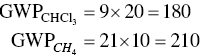
Use of the conversion factors shows that 10 lb of methane has a larger impact on global warming than 20 lb of chloroform.
The key to impact characterization is using the appropriate characterization factor. For some impact categories, such as global warming and ozone depletion, there is a consensus on acceptable characterization factors. For other impact categories, such as resource depletion, a consensus is still being developed. Table 6.1 includes descriptions of possible characterization factors for some of the commonly used life cycle impact categories. A properly referenced LCIA will document the source of each characterization factor to ensure that they are relevant to the goal and scope of the study. For example, many characterization factors based on studies conducted in Europe cannot be applied to American data unless it can be verified that they are appropriate to conditions in the United States.
Step 4: Normalization
Normalization is an LCIA tool used to express impact indicator data in a way that can be compared among impact categories. In this procedure, the indicator results are divided by a reference value selected for the purpose. Reference value may be chosen from among numerous methods.
The following are representatives:
The total emissions or resource use for a given area that may be global, regional, or local.
The total emissions or resource use for a given area on a per capita basis.
The ratio of one alternative to another (i.e. the baseline).
The highest value among all options.
The goal and scope of the LCA may influence the choice of an appropriate reference value. Note that normalized data can only be compared within an impact category. For example, the effects of acidification cannot be directly compared with those of aquatic toxicity because the characterization factors were calculated using different scientific methods.
Step 5: Grouping
Grouping assigns impact categories into one or more sets to facilitate the interpretation of the results into specific areas of concern. Typically grouping involves sorting or ranking indicators. The ISO (1998a) lists two possible ways to group LCIA data:
- Sorting indicators by characteristics such as emissions (e.g. air and water emissions) or location (e.g. local, regional, or global)
- Sorting indicators by a system of ranking based on value choices, such as high, low, or medium priority.
Step 6: Weighting
Weighting (also referred to as valuation) assigns relative values to the different impact categories based on their perceived importance or relevance. Weighting is important because the impact categories should also reflect study goals and stakeholder values. But since weighting is not a scientific process, its methodology must be clearly explained and documented. The weighting stage is the least developed of the impact assessment steps and also is the one most likely to be challenged for integrity. In general, weighting includes the following activities:
Identifying the underlying values of stakeholders
Determining weights to place on impacts
Applying weights to impact indicators
Weighted data should not be combined across impact categories unless the weighting procedure is explicitly documented. The unweighted data should be shown together with the weighted results to ensure a clear understanding of the assigned weights.
In some cases, the impact assessment results are so straightforward that a decision can be made without the weighting step. For example, when the best‐performing alternative is significantly and meaningfully better than the others in at least one impact category and equal to the alternatives in the remaining impact categories, then one alternative is clearly better.
Several issues make weighting a challenge. The first issue is subjectivity. According to ISO 14042, any judgment of preferability is a subjective statement of the relative importance of one impact category over another (ISO 1998a). Additionally, these value judgments may change with location or time of year. For example, a resident of Los Angeles may place more importance on the values for photochemical smog than someone in Cheyenne, Wyoming. The second issue is derived from the first: how should users fairly and consistently make decisions based on environmental preferability, given the subjective nature of weighting? Trying to develop a truly objective (or universally agreeable) set of weights or weighting methods is not feasible. However, several approaches to weighting do exist and are used successfully for decision making.
Step 7: Evaluate and Document the LCIA Results
Now that the impact potential for each selected category has been calculated, the accuracy of the results must be verified. Documentation of the results of the LCIA entails thoroughly describing the methodology used in the analysis, defining the systems analyzed and the boundaries that were set, and setting forth all assumptions on which the inventory analysis was passed.
The LCIA, like all other assessment tools, has inherent limitations, including the following:
- Lack of spatial resolution (e.g. a 4000 gal ammonia release is worse in a small stream than in a large river)
- Lack of temporal resolution (e.g. a 5 T release of particulate matter during a one month period is worse than the same release spread through the whole year)
- Inventory speciation (e.g. broad inventory listing such as “VOC” or “metals” do not provide enough information to accurately assess environmental impacts)
- Threshold and nonthreshold impact (e.g. 10 T of contamination is not necessarily 10 times worse than 1 T of contamination)
The selection of more complex or site‐specific impact models can help reduce the limitations of the impact assessment's accuracy. It is important to document these limitations and to include a comprehensive description of the LCIA methodology, as well as, a discussion of the underlying assumptions, value choices, and known uncertainties in the impact models with the numerical results of the LCIA to be used in interpreting the results of the LCA.
6.2.6 Life Cycle Interpretation
Life cycle interpretation is a systematic technique to identify, quantify, check, and evaluate information from the results of the LCI and the LCIA, and communicate them effectively. Life cycle interpretation is the last phase of the LCA process. The ISO has defined the following objectives of life cycle interpretation:
- Analyze results, reach conclusions, explain limitations, and provide recommendations based on the findings of the preceding phases of the LCA and to report the results of the life cycle interpretation in a transparent manner.
- Provide a readily understandable, complete, and consistent presentation of the results of an LCA study, in accordance with the goal and scope of the study (ISO 1998b).
It is not always possible to use an LCA as the basis for starting, as one alternative is better than the others. This does not imply that efforts have been wasted. Uncertainty in the final results notwithstanding the LCA process still provides decision‐makers with a better understanding of the environmental and health impacts associated with each alternative, where they occur (locally, regionally, or globally), and the relative magnitude of each type of impact potentially attributed to each of the proposed alternatives investigated. This information more fully reveals the pros and cons of the alternatives.
The purpose of conducting an LCA is to better inform decision‐makers by providing a particular type of information (often unconsidered), with a life cycle perspective of environmental and human health impacts associated with each product or process. However, LCA does not take into account technical performance, cost, or political and social acceptance. Therefore, it is recommended that LCA be used in conjunction with these other parameters.
6.2.6.1 Key Steps to Interpreting the Results of the LCA
The guidance provided thus far summarizes the information on life cycle interpretation in the ISO draft standard Environmental Management – Life Cycle Assessment – Life Cycle Interpretation (ISO 1998b). The ISO draft standard covers the following steps in conducting a life cycle interpretation:
- Identify significant issues
- Evaluate the completeness, sensitivity, and consistency of the data
- Draw conclusions and recommendations
Figure 6.5 illustrates the steps of the life cycle interpretation process in relation to the other phases of the LCA process.
Step 1: Identify Significant Issues
Significant “issues” are the data elements that contribute most to the results of both the LCI and LCIA for each product, process, or service. Examples include
- inventory parameters (e.g. energy use, emissions, waste)
- impact category indicators (e.g. resource use, emissions, waste)
- essential contributions for life cycle stages to LCI or LCIA results such as individual unit processes or groups of processes (e.g. transportation, energy production)
When these issues have been identified, the results are used to evaluate the completeness, sensitivity, and consistency of the LCA study (step 2). The identification of significant issues guides the evaluation step.
Before determining which parts of the LCI and LCIA have the greatest influence on the results for each alternative, the previous phases of the LCA (e.g. study goals, ground rules, impact category weights, results, and external involvement, etc.) should be reviewed in a comprehensive manner.
A review of the information collected and the presentations of results developed indicates that if the goal and scope of the LCA study have been met. If they have, the significance of the results can be determined. Several analytical approaches are possible.
- Contribution analysis – The contribution of the life cycle stages or groups of processes are compared to the total result and examined for relevance.
- Dominance analysis – Statistical tools or other techniques, such as quantitative or qualitative ranking (e.g. ABC Analysis), are used to identify significant contributions to be examined for relevance.
- Anomaly assessment – Based on previous experience, unusual or surprising deviations from expected or normal results are observed and examined for relevance.
Step 2: Evaluate the Completeness, Sensitivity, and Consistency of the Data
The evaluation step of the interpretation phase establishes the confidence in and reliability of the results of the LCA. This is accomplished by performing completeness, sensitivity, and consistency checks to ensure that products/processes are fairly compared.

Figure 6.5 Relationship of interpretation steps with other phases of LCA (ISO 1998b).
Completeness check – The completeness check ensures that all relevant information and data needed for the interpretation are available and complete. A checklist should be developed to indicate each significant area represented in the results. Using the established checklist, it is possible to verify that the data comprising each area of the results are consistent with the system boundaries (e.g. all life cycle stages are included) and that the data is representative of the specified area (e.g. accounting for 90% of all raw materials and environmental releases).
The result of this effort will be a checklist indicating that the results for each product/process are complete and reflective of the stated goals and scope of the LCA study. If deficiencies are noted, an attempt must be made to remedy them. If this is not possible because data are not available, areas inadequately characterized because of insufficient data must be highlighted in the final results and their impact on the comparison estimated either quantitatively (percent uncertainty) or qualitatively (alternative A's reported result may be higher because “X” is not included in its assessment).
Sensitivity check – The objective of the sensitivity check is to evaluate the reliability of the results by determining whether the uncertainty in the significant issues identified in step 1 affect the decision‐maker's ability to confidently draw comparative conclusions. Three common techniques for data quality analysis can be used in performing sensitivity checks.
- Gravity analysis – Identifies the data that has the greatest contribution on the impact indicator results.
- Uncertainty analysis – Describes the variability of the LCIA data to determine the significance of the impact indicator results.
- Sensitivity analysis – Measures the extent that changes in the LCI results and characterization models affect the impact indicator results.
Additional guidance on how to conduct a gravity, uncertainty, or sensitivity analysis can be found in the EPA document entitled “Guidelines for Assessing the Quality of Life Cycle Inventory Analysis” (USEPA 1995). If one of these analyses has been conducted as part of the LCI and LCIA phases, these results can be used. Then the sensitivity check will serve to verify that the goals for data quality and accuracy defined early in have been met. If deficiencies exist, additional efforts are required to improve the accuracy of the LCI data collected and/or impact models used in the LCIA. If better data or impact models cannot be obtained, the deficiencies for each relevant significant issue must be reported and its impact on the comparison estimated either quantitatively or qualitatively, as with the completeness check.
Consistency check – The consistency check determines whether the assumptions, methods and data used throughout the LCA process are consistent with the goal and scope of the study, and for each product/process evaluated. Verifying and documenting that the study was completed as intended at the conclusion increases confidence in the final results. A formal checklist should be developed to communicate the results of the consistency check. Table 6.2 lists seven categories and provides examples of inconsistencies that can creep into the data. The goal and scope of the LCA determines which categories should be used.
If, after completion of steps 1 and 2, it is determined that the results of the impact assessment and the underlying inventory data are complete, comparable, and acceptable as bases for drawing conclusions and making recommendations then stop! If any inconsistency is detected, document the role it played in the overall consistency evaluation. Although some inconsistency may be acceptable, depending upon the goal and scope of the LCA, the presence of inconsistencies usually means that it is necessary to repeat steps 1 and 2 until the results are able to support the original goals for performing the LCA.
Table 6.2 Examples of checklist categories and potential inconsistencies.
| Category | Example of inconsistency |
| Data source | Alternative A is based on literature and Alternative B is based on measured data. |
| Data accuracy | For Alternative A, a detailed process flow diagram is used to develop the LCI data. For Alternative B, limited process information was available and the LCI data developed was for a process that was not described or analyzed in detail. |
| Data age | Alternative A uses 1980s era raw materials manufacturing data. Alternative B used a one‐year‐old study. |
| Technological representation | Alternative A is bench scale laboratory model. Alternative B is a full‐scale production plant operation. |
| Temporal representation | Data for Alternative A describe a recently developed technology. Alternate B describes a technology mix, including recently built and old plants. |
| Geographical representation | Data for Alternative A were data from technology employed under European environmental standards. Alternative B uses the data from technology employed under US environmental standards. |
| System boundaries, assumptions, and models | Alternative A uses a Global Warming Potential model based on 500‐year potential. Alternative B uses a Global Warming Potential model based on 100‐year potential. |
Step 3: Draw Conclusions and Recommendations
The objective of this step is to interpret the results of the LCIA (not the LCI) to determine which product/process has the overall least impact on human health and the environment, and/or on one or more specific areas of concern as defined by the goal and scope of the study. Depending upon the scope of the LCA, the results of the impact assessment will return either a list of unnormalized and unweighted impact indicators for each impact category for the alternatives or a single grouped, normalized, and weighted score for each alternative. In the latter case, the recommendation may simply be to accept the product/process with the lowest score. The assumptions underlying the analysis should be borne in minds, however. If an LCIA stops at the characterization stage, the LCIA interpretation is less clear‐cut. The conclusions and recommendations rest on balancing the potential human health and environmental impacts in light of study goals and stakeholder concerns.
It is essential to understand and communicate the uncertainties and limitations in the procedures that have produced the final recommendations. Perhaps no one product or process is better than another because of underlying uncertainties and limitations in the methods used to conduct the LCA. Perhaps insufficient good data were available, or restrictions on time or resources prevented analysts from thoroughly exploring certain aspects of the problem. Even so, the results of the LCA can be used to help inform decision‐makers about the human health and environmental pros and cons and understand the significant impacts of each. Such LCA results will reveal whether effects are occurring locally, regionally, or globally, and will provide at least a rough estimate of the magnitude of each type of impact in comparison to the proposed alternatives being investigated.
6.2.6.2 Reporting the Results
When the LCA has been completed, the materials must be assembled into a comprehensive report documenting the study in a clear and organized manner. This will help communicate the results of the assessment fairly, completely, and accurately to others interested in the results. The report presents the results, data, methods, assumptions and limitations in sufficient detail to allow the reader to comprehend the complexities and trade‐offs inherent in the LCA study.
If the results will be communicated to parties who were not involved in the LCA study (e.g. stakeholders), the report will serve as a reference document, and it can help prevent any misrepresentation of the results.
6.2.6.3 Conclusion
Adding LCA to the decision‐making process provides a level of understanding of human health and environmental impacts that traditionally has not been available to those responsible for selecting a product or process. This valuable information provides a way to account for the full impacts of decisions, especially those made off‐site, that are directly influenced by the selection of a product or process. As emphasized earlier, LCA is a tool to better inform decision‐makers and other decision criteria such as cost and performance must be weighed to reach a well‐balanced decision.
As we have seen, LCA and LCI can be valuable tools in environmental analysis. To make sense of the many large data sets collected in any such study is clearly a task too complex to be undertaken without the assistance of computers. Section 6.3 describes some of the software tools that have been developed for this purpose.
6.3 LCA and LCI Software Tools
Table 6.3 lists the LCA and LCI tools we shall discuss in this section, along with the vendor or developer of each and that organization's Internet address.
6.3.1 ECO‐it 1.0
ECO‐it is a database tool used to assist an LCI and LCIA. ECO‐it comes with over 100 indicator values for commonly used materials such as metals, plastics, paper, board, and glass, as well as production, transport, energy, and waste treatment processes.
6.3.2 EcoManager
EcoManager is LCI tool designed to be used by persons who have or who gain a working knowledge of the LCI methodology for internal planning, screening, and evaluation. EcoManager uses a software program developed by Pira International of the United Kingdom, in combination with US LCI data from the Franklin Associates, Ltd. (FAL) database. Developed for use with Microsoft Excel, EcoManager utilizes spreadsheets and program codes called “macros” to guide the user through the construction of a LCI, access data from the databases, perform file management functions, edit existing and produce graphics and reports. The system provides online help at every stage of operation. The system also provides graphic and report features. And because the program has been created in Excel, all of the power of Excel for graphics, exporting, and file management are available for customized outputs.
6.3.3 Eco Bat 2.1
Eco Bat is an LCIA and design for environment (DfE) tool that models product life cycles with flow chart diagrams. This Windows‐based application offers an online help, a toolbar, and icons, including a large database.
Table 6.3 LCA and LCI software tools.
| Name | Developer/vendor | URL |
| 1. ECO‐it | PRé Consulting | http://www.pre.nl.eco‐it.html |
| 2. EcoManager | Franklin Associates, Ltd | http://www.fal.com/software/ecoman.html |
| 3. EcoPro 1.5 | EcoPerformance Systems, Switzerland | http://www.sinum.com/ |
| 4. Gabi 4 | Institute for Polymer Testing and Polymer Science University of Stuttgart | http://www.pre‐product.de/english/main/software.htm |
| 5. IDEMAT | Delft University of Technology | http://www.io.tudelft.nl/research/mpo/idemat/idemat.htm |
| 6. LCAID | Battelle Memorial Institute/US Department of Energy | http://www.estd.battelle.org/sehsm/lca/LCAdvantage.html |
| 7. LCAiT | Chalmers Industriteknik, Sweden | http://www.ekologik.cit.chalmers.se/lcait.htm |
| 8. REPAQ | Franklin Associates, Ltd. | http://www.fal.com/software/repaq.html |
| 9. SimaPro 7 | PRé Consulting | http://www.pre.nl/simapro.html |
| 10. TEAM | Ecobalance | http://www.ecobalance.com/software/team/team_ovr.htm |
| 11. TRACI | U.S. Environmental Protection Agency | http://www.epa.gov/ORD/NRMRL/std/sab/iam_traci.htm |
| 12. Umberto NXT CO2 | Institute for Energy and Environmental Research Heidelberg, Hamburg GmbH | http://www.ifu.com/software/umberto‐e/ |
6.3.4 GaBi 4
GaBi is a life cycle engineering or life cycle management (LCM) and life‐cycle engineering (LCE) tools that use many predefined data objects from industry and literature. Users can link data sets supplied with the GaBi database to own data in order to calculate both life cycle inventories and impact assessments. It allows clear weak point analyses of inventories and valuated balances. The structure is open to alterations and extensions.
6.3.5 IDEMAT
Idemat is a computer database of over 365 materials from the Department of Environmental Product Development of the faculty of Industrial Design Engineering at the Delft University of Technology. It provides technical information about materials and processes in words, numbers, and graphics, and puts emphasis on environmental information. The program was developed to be used by students of technically oriented academic disciplines like industrial design engineering, civil engineering, material science, and aerospace engineering. Users must be quite familiar with the principles of LCA and the methods for characterization and evaluation of the environmental impacts as published by SETAC and the Center for Environmental Studies at the University of Leiden (CML), and used in SimaPro.
6.3.6 EIOLCA
EIOLCA: The economic input–output life cycle assessment (EIOLCA) model, developed by Carnegie Mellon University, estimates the materials and energy resources required for, and the environmental emissions resulting from, activities in our economy. It is a free, fast, and easy LCA model available online (www.eiolca.net).
6.3.7 LCAD
Life‐cycle advantage, or LCAD5, is a life cycle modeling tool that has a graphical user interface and database structure. LCAD can model process flow diagrams with material and energy balances, and labor and revenue inputs. LCAD can also assess the data reliability. The LCAD system includes a basic commodity database for the United States, covering fuels production and distribution, power generation, and cradle‐to‐gate operations for selected forest products, paper, metals, cement, and basic chemicals and plastics.
6.3.8 LCAiT
LCAiT is a LCI tool that aids in generating an energy and materials balance. LCAiT also contains a cradle‐to‐gate information regarding certain materials.
6.3.9 REPAQ
REPAQ is a LCI software program that permits users to examine energy and environmental emissions for the entire life cycle of a product, beginning with raw material extraction and continuing through refining and processing, material manufacture, product fabrication, and disposal. Products, processes, and packaging can be evaluated with REPAQ. Users may access the REPAQ database and enter their own data through the Custom Materials feature, which allows entry of data for any process for which LCI data can be gathered.
6.3.10 SimaPro 7
SimaPro is a full‐featured LCA software tool that facilitates the comparison and analysis of complex products capable of dealing with complex tools and software: LCM, LCIA, LCI, LCE, substance/material flow analysis (SFA/MFA), DfE, product stewardship, supply chain management, life cycle sustainability (LCS), and life cycle cost (LCC). The process databases and the impact assessment databases can be edited and expanded without limitation. SimaPro can trace the origin of any result that has been implemented. Special features include multiple impact assessment methods, multiple process databases, and automatic unit conversion. SimaPro comes with several well‐known impact assessment methods, including CML, Eco‐points, and the Eco‐indicator method developed by PRé. All impact assessment data can be edited and expanded.
6.3.11 TEAM (Tool for Environmental Analysis and Management)
TEAM is an LCA software program that allows the user to build and use a database and model any system representing the operations associated with products, processes, and activities (waste management options, means of transportation, etc.). It is designed to describe and model complex industrial systems and to calculate the associated life cycle inventories (LCM, SFA/MFA, DfE, DfR), life cycle potential environmental impacts, legal compliance checks, product stewardship, and process‐oriented life cycle costing.
6.3.12 TRACI: A Model Developed by the USEPA
The tool for the reduction and assessment of chemical and other environmental impacts (TRACI) is described along with its history, the research and methodologies it incorporates, and the insights it provides within individual impact categories.
TRACI, a stand‐alone computer program developed by the U.S. Environmental Protection Agency (USEPA), facilitates the characterization of environmental stressors that have potential effects, including ozone depletion, global warming, acidification, eutrophication, tropospheric ozone (smog) formation, ecotoxicity, human health criteria–related effects, human health cancer effects, human health noncancer effects, fossil fuel depletion, and land‐use effects. TRACI was originally designed for use with LCA, but it is expected to find wider application in the future (Bare 2003; USEPA 2003).
6.3.13 Umberto NXT CO2
Umberto is an LCA tool that uses the following instruments: LCM, LCIA, LCI, LCE, a graphical interface to model material flow networks to enter and track material and energy flows, SFA/MFA, supply chain management, LCS, and LCC.
6.3.14 International Organizations and Resources for Conducting Life Cycle Assessment
Appendix F provides a list of organizations in various countries, a brief description of each organization, and LCA centers and societies across all continents including Africa, Asia, Australia and New Zealand, Europe, North America, and South America.
6.4 Evaluating the Life Cycle Environmental Performance of Chemical‐, Mechanical‐, and Bio‐Pulping Processes
6.4.1 Introduction
Pulp and paper manufacturing constitutes one of the largest industry segments in the United States in terms of water and energy usage and total discharges to the environment. More than many other industries, however, this industry plays an important role in sustainable development because its chief raw material – wood fiber – is renewable. This industry provides an example of how a resource can be managed to provide a sustained supply to meet society's current and future needs. The objective of this work is to present streamlined environmental LCA between chemical (kraft–sulfate), mechanical (or thermomechanical), and biopulping processes. This LCA would help us to evaluate the industry's current experience and practices in terms of environmental stewardship, regulatory and nonregulatory forces, life cycles of its processes and products, and future developments.
The pulping industry has been traditionally using mechanical or chemical pulping methods, or a combination of the two, to produce pulps of desired characteristics. Mechanical pulping accounts for about 25% of the wood pulp production in the world today. Mechanical pulping, with its high yield, is viewed as a way to extend the forest resources. However, mechanical pulping is electrical energy–intensive and yields paper with less strength compared to that produced by the chemical pulping process. These disadvantages limit the use of mechanical pulps in many grades of paper. Chemical pulping accounts for about 75% of the wood pulp production in the world. This process produces paper with very high strength. However, the process has the disadvantages of being capital‐ and energy‐intensive, giving relatively low yields, producing troublesome waste products, and producing by‐products that are of relatively low values.
A new technology that offers a biopulping process with the potential to ameliorate some of these problems is being tested on a commercial scale. Biopulping treats wood chips with a natural wood‐decaying fungus before mechanical pulping and can save substantial amounts of electricity, significantly reduce the amount of air pollutants (including CO2 and some odor‐causing total reduced sulfur compounds) and water pollutants (BOD, COD, TSS) compared with conventional pulping, improve paper quality, and enhance economic competitiveness.
The USEPA's TRACI (USEPA 2003) model was used to assess the chemical, environmental, and human health impacts attributed to three pulp and papermaking processes. The results obtained from the biopulping process indicate a significant reduction in environmental and human health impacts. The biopulping process proves to be more sustainable in terms of economic advantage, and environmental and human health benefits.
6.4.2 Application of LCA
LCA is a tool, which has been described in Sections 6.4 and 6.5, for evaluating the environmental performance of a process, product, or activity, starting from raw material extraction, through manufacturing, to use, and final disposal. This is known as a “cradle‐to‐grave” approach (Figure 6.3). Because of its holistic approach to system analysis, LCA is becoming an increasingly important decision‐making tool in environmental system management. Its main advantage over other, site‐specific, methods for environmental analysis, such as environmental impact assessment or environmental audit, lies in broadening the system boundaries to include all burdens and impacts in the life cycle of a product or a process, and not focusing solely on the emissions and wastes generated by the plant or manufacturing site.
As an environmental management tool, LCA has two main objectives. Its first objective is to quantify and evaluate the environmental performance of a process or a product and so help decision‐makers choose between alternative products or processes. Another objective of LCA is to provide a basis for assessing potential improvements of the environmental performance of an existing or newly designed system. This can be of particular importance to engineers and environmental managers because it can advise them on how to modify or design a system to decrease its overall environmental impact. LCA can thus be used both internally by a company or externally by industry, policy makers, planners, educators, and other stakeholders. If the results of LCA are to be used internally by a company, then possible areas where LCA can be useful include, but are not limited to, the following:
- strategic planning or environmental strategy development
- problem solving in the system
- identification of opportunities for, and tracking of, environmental improvements
- process and product design, innovation, improvement, and optimization
External applications of LCAs include uses of LCA as a marketing tool, to support environmental labeling or claims, or informational purposes, or to support policy decisions. LCA, green chemistry, green engineering, design‐for‐environment, industrial ecology, and other emerging areas of chemical engineering and environmental engineering provide greater opportunities for developing sustainable and innovative processes and products (Das and Scott 2003).
In this case study, we focus only on LCA related to three processes: chemical‐, mechanical‐, and biopulping using wood chips. This streamlined LCA approach will help to identify which process is more sustainable by considering environmental impacts, human health and safety, and process economics.
6.4.3 The Pulping Processes
6.4.3.1 Mechanical Pulping
Mechanical pulping, as the name implies, relies on mechanical energy to convert wood to pulp. Current mechanical pulp manufacturing processes constitute several high‐energy grinding and refining systems, including refiner mechanical pulping (RMP) process, the thermomechanical pulping (TMP) process, the chemimechanical pulping process, and the chemithermomechanical pulping process (Someshwar and Pinkerton 1992; Smook 1992). Mechanical pulping accounts for about 25% of the wood pulp production in the world today. Mechanical pulping, with its high yield, is viewed as a way to extend these resources. However, mechanical pulping is electrical energy–intensive and yields paper with lower strength compared with that produced by chemical pulping which are used in the pulping process. Figure 6.6 shows the basic flow diagram for TMP (Smook 1992). TMP is a modification of RMP; it involves steaming the raw material for a short period of time before and during several refining stages. The steaming serves to soften the chips, with the result that the pulp produced has a greater percentage of long fibers and less shives than RPM. Most often, heating and refining are both done under pressure (TMP), but some systems refine under atmospheric pressure. Chemicals are sometime added at the various stages of refining. In the TMP process, the chips are usually steamed under a pressure of 20–40 psi for 2–4 minutes before refining.
Table 6.4 presents an average quantity (in %) of make‐up chemicals that are typically needed for mechanical/thermomechanical pulping (USDA, personal communication). Table 6.5 presents the energy consumption in various operations of TMP and papermaking process (US Pulp and Paper Industry 1988). Table 6.6 shows a range of effluent loads and other environmental impacts of the TMP process (Hynninen 1998; Sundholm 1999). The data from Tables 6.4–6.6 are used to quantify the environmental and human health impacts that will be discussed later in Section 6.4.3.7.
A study by the National Council of the Paper Industry for Air and Stream Improvement (NCASI 1983) on estimating volatile organic compounds (VOCs) are likely to be released along with the steam during the cooking and refining process. The range of VOC emissions can vary between 1.0 and 7.0 lb of carbon per ton of pulp, depending on the wood species. No emissions other than VOC are expected from the mechanical pulping process.
6.4.3.2 Chemical Pulping Processes
The following discussion centers on chemical pulping processes, which supply more than two‐thirds of world's wood pulp. The most widely used chemical pulping process in papermaking is the kraft, or sulfate, process. Other chemical‐pulping processes (mainly using acid sulfite and soda) are sometimes combined with various chemical‐recovery subprocesses. First used over a century ago, these processes now result in recovery of 90% of the inorganics, which are used in the pulping process. Nearly 100% of the dissolved organics are converted to energy. The typical kraft process involves turning logs into wood chips, which are then pulped (Figure 6.7) (Someshwar and Pinkerton 1992). The major steps in chemical pulp and papermaking processes include wood yard operations, pulping, deknotting, washing and screening, chemical recovery, pulp bleaching, pulp drying, and paper making (Smook 1992; Someshwar and Pinkerton 1992). Various gaseous, particulate, liquid, and solid waste streams are produced within a kraft mill (BOD, COD, TSS, NOx, SO2, CO, CO2, PM, TRS, odor, and ash). A wealth of information in the existing literature addresses various treatment methods and pollution prevention and process optimization techniques for these waste streams. Some of the pollution‐prevention advancements and a summary of reduction in total environmental discharges (wastewater, air emissions, and solid and hazardous wastes) from kraft and sulfite mills across the United States over the last 20–25 years are discussed in the literature cited in the reference section (Das 2005; Das and Jain 2001).

Figure 6.6 Basic flow diagram for TMP process.
Source: From Das and Houtman (2004).
Table 6.4 Make‐up chemical, and energy, water, and land use per 1000 T oven dry (OD) pulp and paper production, using chemical‐, mechanical‐, and bio‐pulping.
| Component | Chemical (kraft/sulfite) | Mechanical | Bio‐TMP |
| H2O2 | 0.5% | 2.0% | 2.5% |
| Na2O–SiO2 | — | 2.0% | 2.5% |
| MgSO4 | 0.5% | 0.5% | 0.5% |
| NaOH | 3.0% | 1.0% | 1.5% |
| NaSO4 | 2.5% | — | — |
| O2 | 4.8% | — | — |
| CIO2 | 3.0% | — | — |
| H2SO4 | 1.0% | — | — |
| Corn steep liquor | — | — | 0.5% |
| Energy usea (MJ/1000 T/day OD pulp) | 3.15 × 10⁷ | 8.24 × 10⁷ | 5.25 × 10⁷ |
| Water use (gal/1000 T/day OD pulp) | 1.6 × 10⁷ | 6.0 × 10⁶ | 6.0 × 10⁶ |
| Land use (acre/1000 T/day OD pulp) | 20 | 20 | 25 |
Table 6.4 presents an average quantity (in percentage) of make‐up chemicals that are typically needed for chemical pulping. Chemical pulping uses 63% more chemical than mechanical pulping, and 53% more than biopulping. Table 6.5 presents the energy consumption in various operations of chemical pulping and papermaking processes. Table 6.6 shows a range of effluent loads and other environmental impacts of chemical pulping and papermaking processes. The data from Tables 6.4–6.6 are used to quantify the environmental and human health impacts that will be discussed later in Section 6.4.3.7.
6.4.3.3 Biopulping: A Review of a Pilot Project
Biopulping is the treatment of wood chips and other lignocellulosic materials with lignin‐degrading fungi before pulping. Ten years of industry‐sponsored research has demonstrated the technical feasibility of the technology for mechanical pulping at a laboratory scale. Two 50‐T outdoor chip pile trials conducted at the USDA Forest Service, Forest Products Laboratory (FPL) in Madison, WI, have established the engineering and economical feasibility of the technology. After refining the control and the fungus‐treated chips through a thermomechanical pulp (TMP) mill, the resulting pulps were made into papers on the pilot‐scale paper machine at FPL. In addition to the 30% savings in electrical energy consumption during refining, improvements in the strength of the resulting paper were seen as a result of fungal pretreatment. Because of the stronger paper, we were able to substitute at least 5% kraft pulp in a blend of mechanical and kraft pulps. This recent work has clearly demonstrated that economic benefits can be achieved with biopulping technology through both the energy savings and substitution of the stronger biopulped TMP for more expensive kraft, while maintaining the paper quality.
6.4.3.4 Introduction to Biopulping
Biopulping, which uses natural wood decay organisms, has the potential to overcome these problems. Fungi alter the lignin in the wood cell walls, which has the effect of “softening” the chips. This substantially reduces the electrical energy needed for mechanical pulping and leads to improvements in the paper strength properties. The fungal pretreatment is a natural process; therefore, no adverse environmental consequences are foreseen (Kirk et al. 1993, 1994; Sykes 1994). Based on the results of previous work and discussions with mill personnel, we envision a fungal treatment system that fits into existing mill operations with minimal disturbance. Figure 6.8 is a conceptual overview of the biotreatment process in relation to existing wood yard operations. Wood is harvested and transported to the mill site for debarking, chipping, and screening. Chips are decontaminated by steaming, maintaining a high temperature for a sufficient time to decontaminate the wood chip surfaces, and then cooled so that the fungus can be applied. The chips are then placed in piles that can be ventilated to maintain the proper temperature, humidity, and moisture content for fungal growth and subsequent biopulping. The retention time in the pile is 1–4 weeks. Recent efforts have focused on bringing the successful laboratory‐scale procedures up to the industrial level. Our laboratory process treats approximately 1.5 kg of chips (dry weight basis) at one time. In our scale‐up experiments that took biopulping from this lab scale to larger scales, certain implementations of each step were chosen. The chosen implementation allowed us to reach our two goals for this phase of the project: (i) to demonstrate that chips can be decontaminated and inoculated in a continuous process rather than as a batch process and (ii) to demonstrate that the process scaled as expected from an engineering standpoint. The following discusses the results obtained during the scale‐up trials in relation to industrial processes.
Table 6.5 Summary of specific energy consumption in current pulp and papermaking processes (million Btu/T pulp unless specified otherwise).
| Process | Range of energy variation | ||
| Minimum | Maximum | Typical average | |
| Wood preparation componenta Debarkinga Debarking |
0.16 | 0.25 | 0.19 |
| Chipping | 0.27 | 0.38 | 0.32 |
| Pulping component: Chemical Pulping Digesting |
1.5 | 8.00 | 4.7 |
| Washing | 0.32 | 1.10 | 0.57 |
| Refining/screening | 2.0 | 4.20 | 3.0 |
| Drying | 4.0 | 5.00 | 4.2 |
| Mechanical pulping Stone grinding/refining |
13.2 | 15.20 | 14.5 |
| Mechanical refining | 18.6 | ||
| Thermomechanical refining | 19.6 | 23.10 | 19.7 |
| Wastepaper pulping | 4.0 | 5.82 | 4.3 |
| Bio‐TMP pulping | 13.72 | 16.17 | 13.8 |
| Bleaching component | 1.2 | 14.20 | 7.5 |
| Chemical recovery component Evaporation/concentration |
2.05 | 5.35 | 4.4 |
| Recovery furnace auxiliary | 2.00 | 4.00 | 2.64 |
| Recausticizing | 1.00 | 1.05 | 1.02 |
| Lime kiln | 0.94 | 2.50 | 2.0 |
| Kraft recovered energyb | −4.00 | −20.0 | −15.0 |
| Papermaking componenta Stock preparation |
2.7 | 5.01 | 3.38 |
| Sheet formation | 0.13 | 0.40 | 0.26 |
| Pressing | 0.32 | ||
| Drying | 5.0 | 20.00 | 7.40 |
| Auxiliary componenta Lighting and space heating |
0.42 | 2.00 | 1.68 |
| Power plant | 1.00 | 1.50 | 1.25 |
a Million Btu/T of paper.
b Energy recovered as steam from kraft recovery boiler.
Table 6.6 Effluent loads from the manufacture of forest products.
| Product | Effluent (m3/MT) | Suspended solids (kg/MT) | BOD (kg/MT) | COD (kg/MT) | N (g/MT) | P (g/MT) |
| Pulp Sulfate pulp, unbleached |
20–60 | 12–15 | 5–10 | 20–30 | 200–400 | 80 |
| Sulfate pulp, conventional bleachinga | 60–100 | 12–18 | 18–25 | 60–120 | 300–500 | 120 |
| Sulfate pulp, ECF or TCFb | 30–50 | 10–15 | 14–18 | 25–40 | 400–600 | 100 |
| Sulfite pulp, conventional bleaching | 150–200 | 20–40 | 30–40 | 60–100 | 100–200 | 60 |
| Groundwood, unbleached | 6–10 | 10–30 | 10–15 | 30–50 | 100–200 | 50 |
| TMP, unbleached | 6–15 | 10–30 | 15–25 | 40–80 | 100–200 | 70 |
| TMP, peroxide bleached | 6–5 | 10–30 | 20–40 | 60–100 | 200–300 | 100 |
| Recycled fiber, deinked | 10–20 | 5–10 | 20–40 | 40–80 | 100–200 | 40 |
| Paper and paperboard Fine paper, coated |
30–50 | 10–20 | 3–8 | 10–20 | 50–100 | 5 |
| Newsprint | 10–25 | 5–10 | 1–3 | 2–4 | 10–20 | 5 |
| Folding boxboard | 10–25 | 5–10 | 2–4 | 3–6 | 50–100 | 8 |
| Sack paper | 15–30 | 5–10 | 2–4 | 4–8 | 100–200 | 15 |
| Tissue | 20–40 | 5–10 | 1–3 | 3–6 | 50–80 | 8 |
The figures in the table were compiled from measurements made at Finish mills. ECF, elemental chlorine free; TCF, total chlorine free.
a Kappa number 20–30, depending on wood species.
b Extended cooking, oxygen delignification, kappa number 8–14, depending on wood species.

Figure 6.7 Schematic diagram of a typical kraft‐sulfate pulping and recovery process.
Source: From Someshwar and Pinkerton (1992).
Figure 6.8 Overview of the biopulping process showing how the biotreatment process fits into an existing mill's wood handling systems.
Source: From Das (2005).
In reactor scale‐up studies, Kirk and others (1993) investigated two types of reactor systems: tubular reactors and chip piles. The tubular reactors have an advantage in obtaining the necessary engineering and kinetic data for scaling‐up the process. The one‐dimensional nature of the system is easy to analyze and model. The reactor also allows for well‐controlled air flow in the system with air flow patterns that are well known. Heat loss from the system is easily controlled with exterior insulation, thus achieving conditions that would be experienced in the center of large chip piles. Details on the configurations of these reactors and the chip piles have been published.
6.4.3.5 Large‐Scale Implementation of Biopulping
On a large scale, decontamination and inoculation must be done on a continuous basis and not batchwise as in a laboratory trial (Figure 6.9). To achieve this, the FPL investigators built a treatment system based on two screw conveyers that transport the chips and act as treatment chambers. Figure 6.9 is an overview of the continuous process equipment used in 5‐ and 50‐T trials. Steam is injected into the first screw conveyer, which heats and decontaminates the chip surface. A surge bin, located between the two conveyers, acts as a buffer. From the bottom of the surge bin, a second screw conveyer removes the chips, which are subsequently cooled with filtered air. In the second half of the second screw conveyer, the inoculum suspension containing fungus, unsterilized corn steep liquor, and water is applied and mixed with the chips through the tumbling action. From the screw conveyer, the chips fall into the pile or reactor for a two‐week incubation. In the first scale‐up trial, 5 T of spruce wood chips were inoculated and incubated at a throughput of approximately 0.5 T/h.
In successful outdoor trials with the biopulping fungus Ceriporiopsis subvermispora, nearly 50 T of spruce was treated at a throughput of about 2 T/h (dry weight basis) continuously for over 20 hours. During the two weeks, the chip pile was maintained within the temperature growth range for the fungus, despite the outdoor exposure to ambient conditions.
6.4.3.6 Economics and Environmental Benefits of the Biopulping Process
The economic benefits of biopulping, evaluated based on the process studies and engineering data, result from several effects. Energy reduction at the refiner was used as the primary criterion for the effectiveness of biopulping. For a two‐week process, the savings should be a minimum of 25% under the worst‐case conditions of wood species and minimal process control, whereas up to nearly 40% can be achieved under some circumstances. Additionally, mills that are currently throughput‐limited as a result of refiner capacity may achieve total capacity increases as a result of biopulping. The improved strength of the biomechanical pulps would allow the required strength of the blend to be achieved with a lower percentage of the kraft pulp in those cases where the pulps are blended. Finally, only benign materials are used, and no additional waste streams are generated. An economic analysis of the process yielded very favorable results. The analysis of a 200 T/day TMP mill are summarized here. Under different scenarios and assumptions for utility costs, equipment needs, and operating costs, the net savings can range from $10 to more than $26/T of pulp produced, with an estimated capital investment of $2.5 million. Mills that are refiner‐limited can experience throughput increases of over 30% from the reduction in refining energy by running the refiners to a constant total power load. Even a modest throughput increase of 10%, coupled with the energy savings of 30%, results in a payback in less than 1 year. This is equivalent to a savings of $34/T at a 15% rate of return on capital. Furthermore, many mills blend mechanical pulps and kraft pulps to achieve the optical and strength properties desired. Additional benefits of over $10/T can be realized when the anticipated stronger biopulped TMP is partially substituted for kraft at a 5% rate. The results of a 600 T/day analysis have also been published (Scott et al. 1998a, b). This preliminary analysis is subject to appropriate qualifications. The capital costs are subject to some variability, in particular the costs associated with integrating the new facility into an existing site. The additional advantages of biopulping, including the environmental benefits and pitch reduction, have not been quantified in this report. Finally, much of this analysis is site‐specific, depending on the operating conditions at the particular mill considering incorporating biopulping into its operations.

Figure 6.9 Continuous treatment system to decontaminate, cool, and inoculate wood chips. Wood chips are steamed in the first screw conveyor before being placed into a surge bin. The second screw conveyor then picks up the chips, cools them, and applies the inoculum. Pile Storage and Ventilation.
Source: From Das (2005).
Although the environmental benefits of biopulping for mechanical pulping have not been quantitatively determined in an economic sense, we can discuss the benefits qualitatively. Sykes (1994) determined that there were no environmental problems with the effluent from a biopulping process. In terms of GHGs, there is a net benefit to the biopulping process. The process itself is oxidative, producing carbon dioxide as the fungus metabolizes the various wood components. However, based on the typical generation efficiency of electrical energy, the reduced energy requirements (~30%) significantly lower the overall generation of carbon dioxide when the entire system is analyzed. Finally, in terms of biological issues with using fungi in the wood yard, there are benefits to using the biopulping fungus. The biopulping fungus outcompetes the normal cohort of fungi and other organisms that will grow in an uncontrolled wood chip pile. Some of these other organisms, such as Aspergillis, can be detrimental to human health. The biopulping fungi are naturally occurring in the forests of the world and have no known health effects on humans. More information on benefit–cost analysis and economic input–output model (EIO‐LCA) for chemical process and manufacturing industries are available in Appendix F.
6.4.3.7 Quantitative Analyses Using the USEPA Model: TRACI
The tool for the reduction and assessment of chemical and other environmental impacts (TRACI) is described along with its history, the research and methodologies it incorporates, and the insights it provides within individual impact categories.
TRACI, a stand‐alone computer program developed by the US Environmental Protection Agency (USEPA), facilitates the characterization of environmental stressors that have potential effects, including ozone depletion, global warming, acidification, eutrophication, tropospheric ozone (smog) formation, ecotoxicity, human health criteria–related effects, human health cancer effects, human health noncancer effects, fossil fuel depletion, and land‐use effects. TRACI was originally designed for use with LCA, but it is expected to find wider application in the future (Bare 2003; UNEP‐SETAC 2000).
The categories of odor, noise, radiation, waste heat, and accidents are outside of the USEPA's purview and are usually not included within case studies in the United States for various reasons, including, perhaps, because the perceived threat from these categories is often considered minimal, local, or difficult to predict. The resource depletion categories are recognized as being of significance in the United States, especially for fossil fuel, land, and water use.
For the development of TRACI, each of the above impact categories was considered and its current state of development and perceived societal value were assessed. The traditional pollution categories of ozone depletion, global warming, human toxicology, ecotoxicology, smog formation, acidification, and eutrophication were included within TRACI because various programs and regulations within the USEPA recognize the value of minimizing effects from these categories. The category of human health was further subdivided into cancer, noncancer, and criteria pollutants (with an initial focus on particulates) to better reflect the focus of renewable fuels, and purchased electricity used. Emissions from wastewater treatment plant and other biological processes are not included. In Washington State, 60% energy used in the pulp and paper mills are generated from renewable sources (almost all from hydro) and 40% from purchased electricity generated from natural gas, coal, and oil. The CO2 emissions from renewable energy sources assumed zero. Typical values of 70% combustion efficiency and 60% electricity transmission efficiency were assumed. For an overall efficiency factor of 42% in calculating CO2 emissions from nonrenewable sources, power‐generating plants to pulp mills were used.
USEPA regulations and to allow methodology development consistent with US regulations, handbooks, and guidelines (USEPA 1989b, c). Smog‐formation effects were kept independent and not further aggregated with other human health impacts because environmental effects related to smog formation would have become masked and/or lost in the process of aggregation. Criteria pollutants were maintained as a separate human health impact category, allowing a modeling approach that can take advantage of the extensive epidemiological data associated with these well‐studied impacts.
6.4.3.8 Model Input and Output
It is important to note that data quality is fundamental to LCA and its interpretation. Some of the data quality issues such as reliability and consistency can be overcome by using standardized database, which are starting to emerge after years of data compilation and their incorporation into publicly and commercially available databases. Table 6.7 presents some chemical release data that are used in TRACI. Table 6.8 presents the overall environmental and human health impacts, including global warming, smog formation, human health criteria pollutants, acidification, eutrophication, and ecotoxicity. The results indicate that biopulping has a lower environmental impact than that of the TMP process because of its reduced energy consumption. Biopulping also has a lower impact than that of chemical pulping in all the measures except global warming. One should note that the total CO2 production per ton was the highest for chemical pulping, but because kraft recovery furnaces are fired with lignin derived from the wood, a renewable resource, this contribution to GHGs was assumed to be net zero. Figure 6.10 shows global warming characterization results predicted by TRACI.
These results likely indicate that biopulping is the preferred process when the electrical supply is dominated by renewable energy sources. In cases where the fuel mix for producing electricity is largely fossil fuels, chemical pulping provides a process powered by renewable energy but at a cost of higher hazardous waste emissions.
In conclusion, this streamlined LCA clearly indicates that biopulping in the papermaking process has several advantages over chemical and mechanical processes as follows:
Table 6.7 Emissions from chemical‐, mechanical‐, and bio‐pulping and papermaking processes, 1000 T OD per day.
| Pollutant | Chemical | Mechanical | Bio (TMP) |
| Acetone (lb) | 1.5 × 10³ | — | — |
| BOD (lb) | 4.4 × 10³ | 1.76 × 10³ | 1.76 × 10³ |
| CO2,a (lb) CO (lb) |
3.5 × 10⁶ 5.5 × 10⁴ |
8.0 × 10⁶ 5.5 × 10³ |
5.5 × 10⁶ 5.5 × 10³ |
| Chloroform (lb) | 8.5 × 10² | 7.5 × 10² | 7.5 × 10² |
| COD (lb) | 6.0 × 10³ | 1.0 × 10³ | 5.0 × 10² |
| Ethanol (lb) | 5.0 × 10² | 5.0 × 101 | — |
| H2S (lb) Isoprene (lb) |
2.35 × 10³ 1.0 × 10³ |
— 1.0 × 10³ |
— 1.0 × 10³ |
| Methane (lb) | 8.2 × 10³ | 2.7 × 10³ | 2.7 × 10³ |
| Methanol (lb) | 2.3 × 10³ | 6.0 × 10² | 6.0 × 10² |
| Nitrogen (lb) | 7.5 × 10² | — | — |
| NO2 (lb) NO (lb) |
3.5 × 10⁴ 3.5 × 10⁴ |
1.0 × 10³ 1.0 × 10³ |
5.0 × 10² 5.0 × 10² |
| SO2 (lb) | 1.75 × 10⁴ | — | — |
a CO2 emissions would depend on actual nonrenewable energy sources.
Table 6.8 Environmental and human health impacts characterization results in percentage for chemical‐, mechanical‐, and bio‐pulping processes using TRACI.
| Impacts % | Chemical | Mechanical (TMP) | Bio‐pulping (TMP) |
| Global warming | 21 | 47 | 32 |
| Photochemical smog | 44 | 28 | 28 |
| Acidification | 97 | 2 | 1 |
| Ecotoxicity | 36 | 32 | 32 |
| Human health cancer | 36 | 32 | 32 |
| Human health noncancer | 36 | 32 | 32 |
Figure 6.10 TRACI's global warming characterization for chemical‐, mechanical‐, and bio‐pulping.
Source: From Das and Houtman (2004).
- Reduced electrical energy consumption (at least 30%) over mechanical pulping
- Potential 30% increase in mill throughput for mechanical pulping
- Improve paper strength properties
- The TRACI model indicates a significant reduction in environmental and human health impacts
- The biopulping process proves to be more sustainable in terms of not only economic advantage but also environmental and human health benefits
6.5 Evaluating the Life Cycle Environmental Performance of Two Disinfection Technologies
With increasing emphasis on promoting a sustainable ecological future and concern over introducing toxic chemicals in water, disinfection process design is leaning toward technologies that destroy pathogens while balancing the effects of the disinfected wastewater aquatic biota or on a drinking water supply. Since ultraviolet (UV) irradiation is not a chemical additive, it does not leave or produce toxic by‐product in the wastewater, unlike traditional chlorination and dechlorination processes; therefore, the use of UV does not affect a drinking water supply or the aquatic biota in receiving waters.
The objective of this work is to present streamlined environmental (LCAs) between two competitive disinfection processes: chlorine vs. UV. This section discusses the use of LCA to quantify the environmental and public health benefits of UV disinfection technology as opposed to chlorination and dechlorination methods. LCA tools are used to evaluate the short‐term and long‐term environmental effects of both processes and to select the best sustainable process. Our approach applies environmental LCA to these disinfection processes, incorporating economic criteria and all aspects of the environment: chemical use, electricity use, and releases to water, air, and land.
6.5.1 The Challenge
With increasing emphasis on promoting sound ecological practices and concern over introducing toxic chemicals into water, designs for disinfection processes are increasingly leaning toward technologies that destroy pathogens while balancing the effects of this disinfected wastewater on aquatic biota or a drinking water supply.
In the United States and Canada, the use of ultraviolet light irradiation for the disinfection of wastewater has become the accepted alternative to chlorination or chlorination/dechlorination. There are several reasons for this move away from a proven technology. For example, because of current Uniform Fire Codes, containment requirements for volatile gases like chlorine, and public health concerns, municipalities are limited in the amounts of chlorine that can be stored in a water treatment plant. Moreover, the dechlorination process uses yet another chemical pollutant, sulfur dioxide, to remove chlorine from the effluent before discharged into the receiving water. Thus, and because chlorination/dechlorination of wastewater produces possible carcinogens in addition to destroying aquatic biota in the receiving waters, USEPAs started to look for an alternative wastewater disinfection system.
Various governments, municipalities (Das 2002, 2004; Das and Ekstrom 1999; Ecology 1998; LOTT 1994; USEPA 1986, 1992b), and corporations have sponsored research (Loge et al. 1996; Scheible 1987; Scheible and Forndran 1986; White 2010) that shows that the UV disinfection of wastewater was effective and economical. Another most important development was the parallel flow open channel modular UV system. This new design of the UV system for wastewater in the early 1980s opened up UV disinfection for both the retrofit market and new wastewater treatment plants. To promote a friendlier discharge to the marine environment, designers have begun to prefer alternative disinfection technologies, which emphasize sustainable and clean ecological disinfectants – such a clean technology is UV disinfection.
6.5.2 The Chlorination (Disinfection) Process
Despite the acknowledged advantages of disinfection by means of UV irradiation, however, chlorine continues to be the most widely used chemical for the disinfection of wastewater in the United States and elsewhere. The major advantages of chlorine over alternative disinfectants are cost‐effectiveness, reliability, and efficacy against a host of pathogenic organisms. We turn now to a detailed examination of the chlorination process.
When chlorine (Cl2) is dissolved in freshwater, a mixture of hypochlorous acid (HOCl) and hydrochlorite ion (OCl−) is formed (Eq. 6.2). Chlorine exists predominantly as HOCl below pH 7.6 and as OCl− above pH 7.6. HOCl and/or OCl− is defined as free available chlorine, with the hypochlorous acid being the primary disinfectant.
Mono‐, di‐, and tri‐chloramines (NH2Cl, NHCl2, and NHCl3) are formed when chlorine reacts with nitrogen present in secondary effluent in the form of ammonia. Municipal effluents usually contain all these forms of chlorine in some proportion and taken together they are known as “total residual chlorine” (TRC). Because saltwater contains bromide, the addition of chlorine to saltwater will also form hypobromous acid (HOBr), hypobromous ion (OBr−), and bromamines.
Chlorine is typically supplied as liquefied gas in cylinders. Chlorinators apply gaseous chlorine to a feed stream which is then injected into a mixing zone in the chlorine contact chambers. Initial mixing and effective contact times are essential for good process performance. Generally, contact periods of 15–30 minutes are required at peak flow (USEPA, 1985).
6.5.2.1 Limitations
Although chlorine disinfection is a largely reliable and effective process, it has certain limitations. For examples, chlorine reacts with certain chemicals in the wastewater, leaving only the residual for disinfection. Wastewater components that readily combine with chlorine include reduced iron and sulfur compounds, ammoniated‐nitrogen, organic nitrogen, tannins, uric and humic acid, cyanides, phenols, and unsaturated organics. Cysts of Entamoeba histolytica, Giardia lamblia, and Mycobacterium tuberculosis, some viruses, and eggs of parasitic worms show resistance to chlorine. Consistent disinfection in effluents containing organic nitrogen may pose problems, even when a measured free chlorine residual is present.
6.5.2.2 Human Health and Environmental Impact
Chlorine is toxic to aquatic, estuarine, and marine organisms. An additional hazard is the carcinogenic potential of chloro‐organic compounds. Chlorine gas is potentially toxic when inhaled, and chlorine transport poses a risk (see Section 5.10.5and Tables 5.8 and 5.9). Special handling is required and emergency response plans are required under right‐to‐know regulations for on‐site storage of gaseous chlorine. Chlorine gas and the hypochlorites are also highly corrosive. Chlorine gas concentrations of 15–20 ppm for 30–60 minutes are dangerous; higher concentrations for very brief periods can be fatal. Chlorination can result in the formation of carcinogenic chloro‐organics.
The EPA has established toxicity criteria for TRC in receiving waters. In freshwaters the acute level is 19 mg/l (1‐hour average) and the chronic level is 11 mg/l (4‐day average). The saltwater acute and chronic criteria are 13 mg/l (1‐hour average) and 7.5 mg/l (4‐day average), respectively. Due to the toxicity of chlorine residuals at such low concentrations and the high limit of analytical detection (50–100 mg/l), chlorine induced toxicity in the receiving stream is difficult to control.
6.5.3 Dechlorination with Sulfur Dioxide
In the past decade, concerns over chlorine toxicity and protection of fish and wildlife have led to a dramatic growth in the practice of dechlorination to remove all or part of the chlorine residual and halogenated organics remaining after chlorination. Dechlorination also reduces or eliminates toxicity harmful to aquatic life in receiving waters.
Sulfur dioxide gas successively removes free chlorine, monochloramine, dichloramine, nitrogen trichloride, and polychlorinated compounds. When sulfur dioxide is added to wastewater, the following reactions occur:
(6.3)
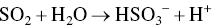
(6.4)

(6.6)

(6.7)

(combined chlorine) (6.8)

For the overall reaction between sulfur dioxide and chlorine (Eq. 6.5), the stoichiometric weight ratio of sulfur dioxide to chlorine is 0.9 : 1. In practice, it has been found that about 1.0 mg/l of sulfur dioxide will accomplish for the dechlorination of 1.0 mg/l of chlorine residue (expressed as Cl2). Because the reactions of sulfur dioxide with chlorine and chloramines are nearly instantaneous, contact time is not usually a factor and contact chambers are not used; however, rapid and positive mixing at the point of application is an absolute requirement.
The ratio of free chlorine to the total combined chlorine residual before dechlorination determines whether the dechlorination process is partial or proceeds to completion. If the ratio is less than 85%, it can be assumed that significant organic nitrogen is present and that it will interfere with the free residual chlorine process (Metcalf and Eddy 2003).
Since dechlorination removes most of the TRC from disinfected wastewaters, it reduces the toxicity of disinfected wastewater effluent to aquatic wildlife. In most situations, sulfur dioxide dechlorination is a very reliable unit process in wastewater treatment, provided the precision of the combined chlorine residual monitoring service is adequate. Excess sulfur dioxide dosages should be avoided not only because of the chemical wastage but also because of the oxygen demand (BOD and COD) exerted by the excess sulfur dioxide.
6.5.3.1 Limitations
Chlorination/dechlorination is more complex to operate and maintain than chlorination alone. Major difficulties are the inability to measure residual SO2 and problems in the continuous measurement of a zero or low chlorine residual. Many halogenated organics are also rapidly formed upon chlorine addition and are unaffected by application of SO2. Heltz and Nweke who examined many plants, reported that the amount of residual chlorine in dechlorinated effluents considerably exceeded EPA criteria for receiving waters (Heltz and Nweke 1995).
6.5.3.2 Environmental Impact
Sulfuric acid and hydrochloric acid are products of SO2 dechlorination in small amounts but are generally neutralized in the wastewater. Based on laboratory experiments, residuals of sulfite dechlorination are at least three orders of magnitude less toxic than chlorine or ozone.
No cases of sulfur compounds affecting dissolved oxygen consumption or pH change in receiving waters or in dechlorinated effluents have been reported. In pilot studies, no significant oxygen depletion occurred until sulfur dioxide overdoses exceeded 50 mg/l. It is not uncommon, however, to find plants with post aeration after dechlorination to assure that dissolved oxygen requirements are met. Dechlorination with SO2 would significantly reduce toxicity due to chlorination disinfection process.
Sulfur dioxide, which is used for dechlorination purposes, is stored on site in small quantities. The maximum anticipated storage inventory is quite small, and there need be no concerns about threats to the health of workers or of residents of nearby populated areas.
6.5.3.3 Effects of Chlorine on Aquatic Life
The potential environmental and chemical effects of chlorine toxicity on 14 aquatic species are summarized in Table 6.9. Rainbow trout was the most sensitive of the species tested, followed by the golden shiner and three‐spined stickleback. A calculated chlorine residual of 0.03 mg/l, based on dilution of a measured concentration of 2.0 mg/l, reduced plankton photosynthesis by more than 20% of the value obtained with a dilution of effluent having no chlorine residual. Dechlorination with sodium bisulfite also eliminated chlorine‐related toxicity. Dechlorination with sulfur dioxide also greatly reduced the acute and chronic toxicity to fish and invertebrate species.
In considering these data, it should be borne in mind that the toxicity of chlorine wastes in rivers depends not on the amount of chlorine added but on the concentration of chlorine remaining in solution (Merkens 1958). The toxicity of this residual chlorine will depend on its composition (i.e. the relative proportions of free chlorine and chloramines). Arriving at this ratio, which in turn depends on at least five other variables, is a complex undertaking. Although free chlorine is more toxic than chloramines, research that has stood since the 1950s suggests that the difference between the toxicity to fish of free chlorine and chloramine is not very great (Dondoroff and Katz 1950; Merkens 1958; Hart 1973; Kozloff 1974).
Table 6.9 Select summary of acute and chronic toxic effects of residual chlorine on aquatic life.
| Species | Effect endpoint | Measured residual chlorine concentration (mg/l) |
| Coho salmon | 7‐day TL50a | 0.083 |
| Pink salmon | 100% kill (1–2) | 0.08–0.10 |
| Coho salmon | 100% kill (1–2) | 0.13–0.20 |
| Pink salmon | Maximum nonlethal | 0.05 |
| Coho salmon | Maximum nonlethal | 0.05 |
| Brook trout | 7‐day TL50 | 0.083 |
| Brook trout | Absent in streams | 0.015 |
| Brown trout | Absent in streams | 0.015 |
| Brook trout | 67% lethality (4) | 0.01 |
| Brook trout | Depressed activity | 0.005 |
| Rainbow trout | 96‐h TL50 | 0.14–0.29 |
| Rainbow trout | 7‐day TL50 | 0.08 |
| Rainbow trout | Lethal (12) | 0.01 |
| Trout fry | Lethal (2) | 0.06 |
| Yellow perch | 7‐day TL50 | 0.205 |
| Largemouth bass | 7‐day TL50 | 0.261 |
| Smallmouth bass | Absent in streams | 0.1 |
| White sucker | 7‐day TL50 | 0.132 |
| Walleye | 7‐day TL50 | 0.15 |
| Black bullhead | 96‐h TL50 | 0.099 |
| Fathead minnow | 96‐h TL50 | 0.05–0.16 |
| Fathead minnow | 7‐day TL50 | 0.082–0.115 |
| Fathead minnow | Safe concentration | 0.0165 |
| Golden shiner | 96‐h TL50 | 0.19 |
| Fish species diversity | 50% reduction | 0.01 |
| Send | Safe concentration | 0.00.34 |
| Send | Safe concentration | 0.012 |
| Daphnia magna | Safe concentration | 0.003 |
| Protozoa | Lethal | 0.1 |
a TL50, median tolerance limit (50% survival) (Brungs 1973).
Results of Laboratory Bioassays
Several studies (Dondoroff and Katz 1950; Merkens 1958; Thatcher 1977) indicated that salmonids were the most sensitive fish species. Laboratory bioassays support this generalization. A residual chlorine concentration of 0.006 mg/l was lethal to trout fry in 2 days, and the 7‐day median tolerance limits, or TL50, for rainbow trout was 0.08 mg/l with an estimated median period of survival of 1 year at 0.004 mg/l (Merkens 1958). The maximum nonlethal (in 23 days) concentration of residual chlorine for pink and coho salmon in seawater was 0.05 mg/l (Holland 1960). Rainbow trout were killed at 0.01 mg/l in 12 days, and they avoided a concentration of 0.001 mg/l (Sprague and Drury 1969). Brook trout had a mean survival time of 9 hours at 0.35 mg/l, 18 hours at 0.08 mg/l, and 48 hours at 0.04 mg/l. Mortality was 67% after 4 days at 0.01 mg/l (Dandy 1967, 1972). Fifty percent of brown trout were killed at 0.02 mg/l within 10.5 hours and at 0.01 mg/l within 43.5 hours (Pike 1971). Trout, salmon, and some fish‐food organisms are more sensitive than warm‐water fish, snails, and crayfish (Tables 6.9 and 6.10).
6.5.4 UV Disinfection Process
A UV disinfection system transfers electromagnetic energy from a mercury arc lamp to an organism's genetic material, the chromosomes which contain DNA and RNA. When UV radiation penetrates the cell wall of an organism, it destroys the cell's ability to reproduce. In the disinfection process, UV radiation, generated by an electrical discharge through mercury vapor, penetrates the genetic material of microorganisms and causes molecular rearrangements that retard their ability to reproduce. Das gave a detailed review of the mechanisms of germicidal action, how does UV light works, how UV‐damaged DNA is repaired, and the effects of wastewater quality parameters on disinfection efficiency (Das 2004).
Table 6.10 Summary of results of brief exposures of fish to residual chlorine.
| Species | Effect endpoint | Time | Measured residual chlorine concentration (mg/l) |
| Chinook salmon | First death | 2.2 h | 0.25 |
| Brook trout | Median mortality | 90 min | 0.5 |
| Brook trout | Mean survival time | 9 h | 0.35 |
| Brook trout | Mean survival time | 18 h | 0.08 |
| Brook trout | Mean survival time | 48 h | 0.04 |
| Brown trout | Depressed activity | 24 h | 0.005 |
| Rainbow trout | Slight avoidance | 10 min | 0.001 |
| Rainbow trout | Lethal | 2 h | 0.3 |
| Fingerling Rainbow trout | Lethal | 4–5 h | 0.25 |
| Trout fry | Lethal | Instantly | 0.3 |
| Yellow perch | TL50a | 1 h | <0.88 |
| Yellow perch | TL50 | 12 h | 0.494 |
| Smallmouth bass | Median mortality | 15 h | 0.5 |
| White sucker | Lethal | 30–60 min | 1.0 |
| Largemouth bass | TL50 | 1 h | <0.74 |
| Largemouth bass | TL50 | 12 h | 0.365 |
| Fathead minnow | TL50 | 1 h | <0.79 |
| Fathead minnow | TL50 | 12 h | 0.26 |
| Miscellaneous | Initial kill | 15 min | 0.28 |
| Miscellaneous | Erratic swimming | 6 min | 0.09 |
a TL50, median tolerance limit (50% survival) (Brungs 1973).
UV disinfection systems are not mass‐produced. Because their efficiency strongly depends on effluent characteristics that act to decrease the UV intensity in wastewater, each application must have a custom‐designed system. Table 6.11 shows the major parameters that must be taken into consideration when a UV disinfection system is being designed for wastewater. In comparison to chlorination/dechlorination, UV disinfection offers a reduction of potential chlorinated hydrocarbons (including potential carcinogens) in the receiving waters, as well as considerably greater safety to wastewater treatment plant operators and to nearby populated areas.
6.5.4.1 UV Transmission or Absorbance
UV light's ability to penetrate wastewater is measured in a spectrophotometer at the same wavelength (254 nm) that is produced by germicidal lamps. This measurement is called the percent transmission or absorbance and it is a function of all the factors that absorb or reflect UV light. As the percent transmission gets lower (higher absorbance) the ability of the UV light to penetrate the wastewater and reach the target organisms decreases.
It cannot be estimated by simply looking at a sample of wastewater with the naked eye. The range of effective transmittances (T) will vary depending on the secondary treatment systems. In general, suspended growth‐treatment processes produce effluent with T varying from 60 to 65%. Fixed film processes range from 50 to 55% T and lagoons 35–40% T. Industries that influence UV transmittance include textile, printing, pulp and paper, food processing, meat and poultry processing, photo developing, and chemical manufacturing. A discussion on other major parameters affecting the UV disinfection efficiency of wastewater is given by Das (2004).
6.5.4.2 Disinfection Standards
The level of disinfection required to obtain an EPA National Pollutant Discharge Elimination System (NPDES) permit is commonly less than 200 fecal coliform unit per 100 ml as a 30‐day geometric mean. In general, a UV dose of 20–30 mW·s/cm2 is required to achieve this level of disinfection in secondary‐treated wastewater with a 65% transmittance and total suspended solids (TSS) below 20 mg/l. The UV dose requirement to meet specific limits depends on the nature of the particle with respect to numbers, size, and composition. Therefore, UV dose requirements will vary (Table 6.11). A more stringent limit (<2.2 total coliform units per 100 ml) is required for water reuse in California and Hawaii. In such cases, filtered effluents with TSS of 2 mg/l or less and 65% transmittance may require UV dose as high as 120 mW·s/cm2 to achieve this level of disinfection. The concentrations of solids, bacteria in the particles, and the particle size distribution are the main limiting factors in the design of systems that must meet stringent disinfection limits. It appears that the UV dose required to achieve the traditional coliform limits will achieve better virus inactivation than the comparable chlorine dose. Figure 6.11, which illustrates the relative doses of UV and chlorine required to inactivate selected organisms compared to fecal coliform indicator, also shows that the chlorine doses required to inactivate most organisms are much higher than comparable UV doses that would achieve the same level of disinfection (Das 2002, 2004; Trojan Technologies Inc. 2010).
Table 6.11 Major parameters affecting the UV disinfection of wastewater.
| Parameters | Acceptable values/conditions |
| Percent transmittance (T) or absorbance | 35–65 |
| Total suspended solids (TSS) mg/L | 5–10 |
| Particle size distribution (PSD) μm | 10–40 |
| Flow rate or hydraulics design | Ideal plug flow |
| Iron (mg/l) | <0.3 |
| Hardness (mg/l) | <300 |
6.5.4.3 Operation, Maintenance, and Worker Safety
The proper operation and maintenance (O&M) of a UV disinfection system ensures that sufficient UV radiation is transmitted to the organisms to render them sterile. All surfaces between the UV radiation and the target organisms must be cleaned, and the ballasts, lamps, and reactor must be functioning at peak efficiency. Inadequate cleaning is one of the most common causes of a UV system's ineffectiveness. In all cases, the quartz sleeves or Teflon tubes need to be cleaned regularly by mechanical wipers, ultrasound equipment, or chemicals. The cleaning frequency is very site‐specific: some systems needing to be cleaned more often than others.
Chemical cleaning is most commonly done with citric acid. Other cleaning agents include mild vinegar solutions and sodium hydrosulfite. A combination of cleaning agents should be tested to find the agent most suitable for the wastewater characteristics without producing harmful or toxic by‐products.
UV is generated on‐site and poses no significant safety concerns to surrounding communities. Worker safety requirements are directed to protection from exposure (primarily of the eyes to skin) from UV light, as well as to strict monitoring of electrical hazards and safe handling and disposal of expended lamps, quartz, and ballasts (US EPA 1996; US EPA 1998).

Figure 6.11 Comparison of the relative effectiveness of chlorine and UV on bacteria and viruses. (i) Escherichia coli (ii) Salmonella typhosa (iii) Staphylococcus aureus (iv) polio virus type 1 (v) Coxsackie AZ virus (vi) adenovirus type (Das 2002, 2004; Trojan Technologies Inc. 2010).
6.5.4.4 Costs
Specifically, consideration must be given to how environmental matters affect our economic thinking and, conversely, how economic decisions affect the environment. Cost considerations are an integral part of the decision‐making process at the stage of identifying potential improvements to a process, a product, or an activity.
Estimated capital costs for 1, 10, and 50 million gal per day (mgd) (1 mgd = 3785 m3/day) plants are $150 000, $700 000, and $3 000 000 respectively. O&M costs are estimated to be 2.6, 1.4, and 0.8 US cents/1000 gal (or 3.785 m3), respectively, at an average dose of 6 mg/l. These increase to 4.0, 3.0, and 1.5 US cents/1000 gal at a dose of 10 mg/l.
Chemical costs of chlorine gas and hypochlorite vary considerably depending upon the locality, demand, and availability. Current prices for Cl2 are varying in the range: $0.0425–0.06/lb (or 454 g) for 90 T (or ~90 000 kg) tank cars; $0.10/lb for 55 T (or ~55 000 kg) rail cars; $0.25–0.275/lb for 1 T (or ~1 000 kg) cylinders; and $0.50–0.55/lb for 150 lb (or ~68 kg) cylinders. Liquid sodium hypochlorite (12.5%) prices quoted were $0.50–1.75/gal.
A brief cost analysis for both chlorination/dechlorination and UV disinfection processes treating a wastewater treatment facility is presented in Figure 6.12, capable of processing 18 mgd. These costs can vary considerably depending on the locality, demands, and supply. The annualized cost values for alternatives were based on the design average plant flow of 18 mgd over a 20‐year period and 5.5% interest rate (F. Soroushian, personal communication; Temmer et al. 2000).
Figure 6.12 indicates that, although the construction cost for chlorination system is considerably less than the UV, annualized costs are about the same for both systems. There is no more real economic benefit for pursuing chlorination disinfection system.
6.5.4.5 Environmental Impacts of Energy Sources and Implications of Renewables
Like chlorination, UV disinfection systems demand energy supplies. One of the most important factors that can contribute to achieving sustainable development is the requirement for a supply of energy resources that is itself fully sustainable. Effective and efficient utilization of energy resources calls for such resources to be readily available at reasonable cost utilized for all required tasks without causing negative societal impact. Clearly, there is an intimate connection between renewable energy sources and sustainable development (Das 2002).
Table 6.12 gives a brief summary of cost of generating powers, air quality, and environmental impacts of renewable and other forms of energy sources. It illustrates that renewable energy sources can make a significant contribution to reducing greenhouse and acid gas emissions. Renewable sources have their own environmental impacts but these are often small, site‐specific, and local in nature.
Figure 6.12 Disinfection system cost comparison of an 18‐mgd facility.
Table 6.12 Cost of generating power, and air quality and environmental impacts.
Source: Energy Ideas Clearinghouse (2018).
| Source | Cost | Potential environmental impact and pollutants of concern |
| Solar photovoltaic (large scale) | ~18–20 US cents/kWh | Corrosive acid, potentially toxic and hazardous substance, land use and loss of habitat, visual intrusion, uncontrolled dumping in landfills |
| Solar photovoltaic (small scale) | ~22–24 US cents/kWh | Potentially toxic and hazardous substance |
| Wind | ~4.5–10 US cents/kWh | Land use and habitat damage, noise, bird strike |
| Biomass | ~6–8 US cents/kWh excluding ethanol‐based fuels | CO2, NOx, PM10, CO, VOC, toxic air pollutants (TAPs) |
| Geothermal | ~5–8 US cents/kWh | Emission of H2S during operation, groundwater and soil contamination, surface water, land use, visual impact |
| Solar thermal | ~5–25 US cents/kWh | Thermal or chemical pollution of surface water |
| Large‐scale hydro | Ranges from 2.0 to 7.8 US cents/kWh | Fish and other aquatic lives, terrestrial ecosystems, local climate, public health, water flow and supply, population displacement, loss of agricultural land |
| Existing hydro | ranges from to 2.0 US cents/kWh | Fish and other aquatic lives, water supply, irrigation, SO2 |
| Nuclear | 5.5–6.0 US cents/kWh | Radioactive substance, public health |
| Coal‐fired generators | 4.8–5.5 US cents/kWh | CO2, NOx, SO2, PM10, CO, VOC, TAPs |
| Diesel generators | 10–15 US cents/kWh | CO2, NOx, SO2, PM10, CO, VOC, TAPs |
| Natural gas combined Cycle combustion turbine |
(at natural gas price of $5/MMBtu) = 5 US cents/kWh | CO2, NOx, PM10, CO, VOC, TAPs |
| Simple cycle combustion turbine | 6 US cents/kWh at $5/MMBtu for natural gas | CO2, NOx, PM10, CO, VOC, TAPs |
6.6 Case Study: LCA Comparisons of Electricity from Biorenewables and Fossil Fuels
A series of LCAs was conducted on biomass, coal, and natural gas systems to quantify the environmental benefits and drawbacks of each. All those evaluations were conducted in a cradle‐to‐grave manner to cover all processes necessary for the operation of the power plant including raw material extraction, feed preparation, transportation, waste disposal, and recycling. We summarize data on energy balance, GWP, air emissions, and resource consumption for each system (NREL 2011).
The generation of electricity and the consumption of energy in general result in consequences to the environment. Using renewable resources and incorporating advanced technologies such as integrated gasification combined cycle (IGCC) may result in less environmental damage, but to what degree, and with what trade‐offs? LCA studies have been conducted on various power generating options in order to better understand the environmental benefits and drawbacks of each technology.
Material and energy balances were used to quantify the emissions, energy use, and resource consumption of each process required for the power plant to operate. These include feedstock procurement (mining coal, extracting natural gas, growing dedicated biomass, collecting residue biomass), transportation, manufacture of equipment and intermediate materials (e.g. fertilizers, limestone), construction of the power plant, decommissioning, and any necessary waste disposal.
The following systems were studied:
- A biomass‐fired IGCC system using a biomass energy crop (hybrid poplar)
- A pulverized coal (pc) boiler with steam cycle, representing the average for coal‐fired power plants in the United States today
- A system cofiring biomass residue with coal (15% by heat input will be presented here)
- A direct‐fired biomass power plant using biomass residue (urban, primarily)
- A natural gas combined cycle (NGCC) power plant.
Each study was conducted independently and can therefore stand alone, giving a complete picture of each power generation technology. However, the resulting emissions, resource consumption, and energy requirements of each system can ultimately be compared, revealing the environmental benefits and drawbacks of the renewable and fossil‐based systems.
6.6.1 Results
6.6.1.1 System Energy Balance
The total energy consumed by each system includes the fuel energy consumed plus the energy contained in raw and intermediate materials that are consumed by the systems. Examples of the first type of energy use are the fuel spent in transportation and fossil fuels consumed by the fossil‐based power plants. The second type of energy is the sum of the energy that would be released during combustion of the material (if it is a fuel) and the total energy that is consumed in delivering the material to its point of use. Examples of this type of energy consumption are the use of natural gas in the manufacture of fertilizers and the use of limestone in flue‐gas desulfurization (FGD). The combustion energy calculation is applied where nonrenewable fuels are used, reflecting the fact that the fuel has a potential energy that is being consumed by the system. The combustion energy of renewable resources, those replenished at a rate equal to or greater than the rate of consumption, is not subtracted from the net energy of the system. This is because, on a life cycle basis, the resource is not being consumed. To determine the net energy balance of each system, the energy used in each process block is subtracted from the energy produced by the power plant. The total system energy consumption by each system is shown in Table 6.13.
To examine the process operations that consume the largest quantities of energy within each system, two energy measurement parameters were defined. First, the energy delivered to the grid divided by the total fossil‐derived energy consumed by each system was calculated. This measure, known as the net energy ratio, is useful for assessing how much energy is generated for each unit of fossil fuel consumed. The other measure, the external energy ratio, is defined to be the energy delivered to the grid divided by the total non‐feedstock energy to the power plant. That is, the energy contained in the coal and natural gas used at the fossil‐based power plants is excluded. The external energy ratio assesses how much energy is generated for each unit of upstream energy consumed.
Table 6.13 Total system energy consumption.
Source: From NREL (2011).
| System | Total energy consumed (kJ/kWh) |
| Average coal | 12 575 |
| Natural gas IGCC | 8 377 |
| Biomass/coal cofiring (15% by heat input) | 10 118 |
| Biomass‐fired IGCC using hybrid poplar | 231 |
| Direct‐fired biomass power plant using biomass residue | 125 |
Because the energy in the biomass is considered to be both generated and consumed within the boundaries of the system, the net energy ratio and external energy ratio will be the same for the biomass‐only cases (biomass‐fired IGCC and direct‐fired biomass). In calculating the external energy ratio, we are essentially treating the coal and natural gas fed to the fossil power plants as renewable fuels, so that upstream energy consumption can be compared. The energy results for each case studied are shown in Figure 6.13.
As expected, the biomass‐only plants consume less energy overall, since the consumption of nonrenewable coal and natural gas at the fossil plants results in net energy balances of less than one. The direct‐fired biomass residue case delivers the most amount of electricity per unit of energy consumed. This is because the energy used to provide a usable residue biomass to the plant is fairly low. Despite its higher plant efficiency, the biomass IGCC plant has a lower net energy balance than the direct‐fired plant because of the energy required to grow the biomass as a dedicated crop. Residue resource limitations, however, may necessitate the use of energy crops in the future. Cofiring biomass with coal slightly increases the energy ratios over those for the coal‐only case, even though the plant efficiency was derated by 0.9 percentage points.

Figure 6.13 Life cycle energy balance.
In calculating the external energy ratios, the feedstocks to the power plants were excluded, essentially treating all feedstocks as renewable. Because of the perception that biomass fuels are of lower quality than fossil fuels, the external energy ratios for the fossil‐based systems were expected to be substantially higher than those of the biomass‐based systems. The opposite is true, however, due to the large amount of energy that is consumed in upstream operations in the fossil‐based systems. The total non‐feedstock energy consumed by the systems is shown in Table 6.14. In the case of coal, 35% of this energy is consumed in operations relating to flue‐gas cleanup, including limestone procurement. Mining the coal consumes 25% of this energy, while transporting the coal is responsible for 32%. Greater than 97% of the upstream energy consumption related to the natural gas IGCC system is due to natural gas extraction and pipeline transport steps, including fugitive losses. Although upstream processes in the biomass systems also consume energy, shorter transportation distances and the fact that FGD is not required reduce the total energy burden.
Table 6.14 Non‐feedstock energy consumption.
Source: From NREL (2011).
| System | Total energy consumed (kJ/kWh) |
| Average coal | 702 |
| Natural gas IGCC | 1718 |
| Biomass/coal cofiring (15% by heat input) | 614 |
| Biomass‐fired IGCC using hybrid poplar | 231 |
| Direct‐fired biomass power plant using biomass residue | 125 |
6.6.1.2 Global Warming Potential
Figure 6.14 shows the net emissions of the three GHGs quantified for these studies: carbon dioxide (CO2), methane (CH4), and nitrous oxide (N2O). The biomass IGCC system has a much lower GWP than the fossil systems because of the absorption of CO2 during the biomass growth cycle. Sensitivity analyses demonstrated that even moderate amounts of soil carbon sequestration (1900 kg/ha/7‐year rotation) would result in the biomass IGCC system having a zero‐net GHG balance. Sequestration amounts greater than this would result in a negative release of GHGs, and a system that removes carbon from the atmosphere overall.
Figure 6.14 Net GHG emission.
The base case presented here assumes no net change in soil carbon, since actual gains and losses will be very site specific. The direct‐fired biomass system in which the residue is used at the power plants has a highly negative rate of GHG emissions because the generation of methane associated with biomass decomposition is avoided. Based on current disposal practices, it was assumed that 46% of the residue biomass used in the direct‐fired and cofiring cases would have been sent to a landfill and that the remainder would end up as mulch and other low‐value products. Decomposition studies reported in the literature were used to determine that if the biomass residue had not been used at the power plant, approximately 9% of the carbon would have ended up as CH4 and 61% as CO2. The remaining carbon is resistant to decomposition in the landfill. Had all the residue biomass been decomposed aerobically, the CO2 produced would have been 1.85 kg/kg biomass. If the biomass residue was not used at the power plant, the decomposition pathways described above would have resulted in total GHG emissions of 2.48 kg CO2‐equiv/kg biomass (1.117 kg CO2 + 0.065 kg CH4). The net difference is the reason for the negative GHG emissions associated with the direct‐fired system.
The NGCC plant has the lowest GWP of all fossil systems because of its higher efficiency, despite natural gas losses that increase net CH4 emissions. Natural gas losses during extraction and delivery were assumed to be 1.4% of the gross amount extracted. Because of the potency of methane as a GHG, nearly one‐quarter of the total GWP of this system is due to these losses. Cofiring biomass with coal at 15% by heat input reduces the GWP of the average coal‐fired power plant by 18%. The reduction in GHGs is greater than the rate at which biomass is cofired because of the avoidance of methane emissions associated with decomposition that would have occurred had the biomass not been used at the power plant. Biomass disposal and decomposition emissions for this scenario are the same as those used in the direct‐fired case.
6.6.1.3 Air Emissions
Figure 6.15 charts the following emissions: particulates, oxides of sulfur (SOx), oxides of nitrogen (NOx), CH4, CO2, and non‐methane hydrocarbons (NMHCs). Methane emissions are high for the natural gas case due to natural gas losses during extraction and delivery. The direct‐fired biomass and coal/biomass cofiring cases have negative methane emissions due to avoided decomposition processes (landfilling and mulching). CO and NMHCs are higher for the biomass case because of upstream diesel combustion during biomass growth and preparation. Cofiring reduces the coal system air emissions by approximately the rate of cofiring, with the exception of particulates, which are generated during biomass chipping and handling.
Figure 6.15 Emissions of PM, SOx, NOx, CH4, CO, and NMHCs.
6.6.1.4 Resource Consumption
Figure 6.16 shows the total amount of nonrenewable resources consumed by the systems investigated. Limestone is used in significant quantities by the coal‐fired power plants for FGD. The natural gas IGCC plant consumes almost negligible quantities of resources, with the exception of the feedstock itself, including that lost during extraction and delivery.
6.6.2 Sensitivity Analysis
A sensitivity analysis was conducted on each system to determine which parameters had the most influence on the results and to pinpoint opportunities for reducing the environmental burden of the system. In general, parameters associated with increasing the system efficiency and reducing the fossil fuel usage had the largest effects. Additionally, for the biomass systems, variables associated with growing a dedicated feedstock and factors affecting how much CO2 and CH4 are avoided by using biomass residue significantly affected the GWP of the system. Overall, however, the sensitivity analyses demonstrated that the conclusions that can be drawn from these studies remain relatively constant as different parameters are varied.
6.6.3 Summary and Conclusions
It is evident that biomass power systems reduce the environmental burden associated with power generation. The key comparative results can be summarized as follows:
- The GWP of generating electricity using a dedicated energy crop in an IGCC system is 4.7% of that of an average US coal power system.
Figure 6.16 Total amount of nonrenewable resources consumed by the systems.
- Cofiring residue biomass at 15% by heat input reduces the GHG emissions and net energy consumption of the average coal system by 18 and 12%, respectively.
- The life cycle energy consumption of the coal and natural gas systems are significantly lower than those of the biomass systems because of the consumption of nonrenewable resources.
- Not counting the coal and natural gas consumed at the power plants in these systems, the net energy consumption is still lower than that of the biomass systems because of energy used in processes related to flue‐gas cleanup, transportation, and natural gas extraction and coal mining.
- The biomass systems produce very low levels of particulates, NOx, and SOx, compared to the fossil systems.
- System methane emissions are negative when residue biomass is used because of avoided decomposition emissions.
- The biomass systems consume very small quantities of natural resources compared to the fossil systems.
- Other than natural gas, the natural gas IGCC consumes small amounts of resources.
These results demonstrate that overall, biomass power provides significant environmental benefits over conventional fossil‐based power systems. In particular, biomass systems can significantly reduce the amount of GHGs that are produced, per kilowatt‐hour of electricity generated. Additionally, because the biomass systems use renewable energy instead of nonrenewable fossil fuels, they consume very small quantities of natural resources and have a positive net energy balance. Cofiring biomass with coal offers an opportunity to reduce the environmental burdens associated with the coal‐fired power systems that currently generate over half of the electricity in the United States. Finally, by reducing NOx, SOx, and particulates, biomass power can improve local air quality over coal‐fired power generation.
6.7 Best Available Control Technology (for Environmental Remediation)
6.7.1 What Is “Best Available Control Technology”?
Best available control technology (BACT) is a pollution control standard mandated by the Clean Air Act:
…an emission limitation based on the maximum degree of reduction of each pollutant subject to regulation under this Act emitted from or which results from any major emitting facility, which the permitting authority, on a case‐by‐case basis, taking into account energy, environmental, and economic impacts and other costs, determines is achievable for such facility through application of production processes and available methods, systems, and techniques, including fuel cleaning, clean fuels, or treatment or innovative fuel combustion techniques for control of each such pollutant.
The USEPA determines what air pollution control technology will be used to control a specific pollutant to a specified limit. When a BACT is determined, factors such as energy consumption, total source emission, regional environmental impact, and economic costs are taken into account. It is the current EPA standard for all polluting sources that fall under the New Source Review (NSR) and PSD permitting guidelines, and is determined on a case‐by‐case basis. The BACT standard is significantly more stringent than the reasonably available control technology standard but much less stringent than the lowest achievable emissions rate standard (U.S. EPA, 2016a).
6.7.1.1 Reasonably Available Control Technology
Reasonably available control technology (RACT) is a pollution control standard created by the EPA and is used to determine what air pollution control technology will be used to control a specific pollutant to a specified limit. RACT applies to existing sources in areas that are not meeting national ambient air quality standards on controlled air pollutants and is required on all sources that meet these criteria. The RACT standard is less stringent than the BACT.
6.7.1.2 Lowest Achievable Emissions Rate
The lowest achievable emissions rate (LAER) is used by the EPA to determine if emissions from a new or modified major stationary source are acceptable under SIP guidelines. LAER standards are required when a new stationary source is located in a non‐attainment air‐quality region (see Figure 4.14). It is the most stringent air pollution standard above the best available control technology and reasonably available control technology standards.
6.7.1.3 Life Cycle‐Based Environmental Law
Life cycle concepts are increasingly becoming a part of environmental regulation, especially those involving GHG emissions. Now LCA is often used in writing about carbon accounting. In these times of heightened concern over climate change, individuals, organizations, and governmental agencies alike are eager to measure the release and impact of GHGs. For example, a variety of governmental agencies are developing approaches for regulating the emissions of GHGs associated with the production and use of fuels. As an example, the Energy Independence and Security Act (HR 6) of 2007 (EISA 2007) aims to: move the United States toward greater energy independence and security; increase the production of clean renewable fuels; protect consumers; increase the efficiency of products, buildings, and vehicles. States are also implementing GHGs emission regulation (USEPA 2010). For example, California Global warming Solutions Act of 2006 resulted in regulations that establish a limit for life cycle GHG emissions of transportation fuels. Both the California low‐carbon fuel standard and Section 526 of EISA require a life cycle evaluation of the GHG emissions of transportation fuels and this is becoming a common approach to considering GHG emissions (Allen et al. 2009).
6.7.1.4 Life Cycle Best Control Technology
A number of quantitative tools are emerging that enable life cycle assessments and analyses, and subsequently provide guidance on selecting best available control technologies for PSD, NPDES, and other environmental permitting processes. Many of our environmental laws are based on risk frameworks. Now, the life cycle–based best control technology decisions in environmental permitting processes are made that incorporate not only health and environmental but also the economic and societal impacts. Next, we present a case study on BACT for a power‐generating facility.
6.8 BACT: Applications to Gas Turbine Power Plants
In the United States, BACT comprises the equipment and methods needed to achieve the maximum degree of reduction of pollutants subject to federal regulations that are emitted from any proposed major stationary source or major modification of such a source. The pollutants subject to review under the PSD regulations, and for which a BACT analysis is required, include nitrogen oxides (NOx), carbon monoxide (CO), particulates less than or equal to 10 μm in diameter (PM10), and VOC. All PM is assumed to be PM10. The BACT review follows the “top‐down” approach recommended by the USEPA. The top‐down process calls for all available control technologies for a given pollutant to be identified and ranked in descending order of control effectiveness. The permit applicant should first examine the highest‐ranked (“top”) option. The top‐ranked options should be established as BACT unless the permit applicant demonstrates to the satisfaction of the permitting authority that technical consideration, or energy, environmental, or economic impacts justify a conclusion that the top‐ranked technology is not “achievable” in that case. If the most effective control strategy is eliminated in this fashion, then the next most effective alternative should be evaluated, and so on, until an option is selected as BACT.
The USEPA has broken down this analytical process into the following five steps:
- Step 1: Identify all available control technologies
- Step 2: Eliminate technically infeasible options
- Step 3: Rank remaining control technologies
- Step 4: Evaluate most effective controls and document results
- Step 5: Select the BACT
If there is no single BACT for any industry, it is determined on a case‐by‐case basis, taking into account cost‐effectiveness, economic, energy, environmental, and other effects of proposed solutions. Three important terms in BACT analysis are PSD, “significant emission rate” (SER), and ambient air quality analysis and national ambient air quality standards (NAAQS). The purpose of the PSD program is to implement the Federal Clean Air Act requirements for the prevention of “significant” deterioration of air quality. These insure that the permitting of proposed new industrial facilities and the associated economic growth will occur in a manner consistent with the preservation of clean air resources. The program provides for special emphasis on implementation of BACT, protecting of scenic areas such as national park, and informed public participation. SER refers to net emissions increase or the potential of a source to emit pollutants, a SER equal to or greater than the rates listed in Title 40 CFR 51. An ambient air quality analysis must be carried out for each regulated pollutant and must demonstrate that the source will not cause nor contribute to a violation of any applicable NAAQS.
As industries age and expand, they acquire new emissions units for pollutants and modify old ones. Federal law calls for a BACT analysis of each such new or altered unit of “major stationary sources.” Major stationary source, as defined in Title 40 CFR Part 51, Subpart 1, review of new sources and modification – any stationary source that (1) emits, or has the potential to emit (PTE), 250 T/Y or more of any pollutant under the CAA; or (2) emits, or has the PTE, 100 tpy or more of a regulated pollutant within one of the 28 sources categories (Title 40 CFR).
The USEPA has consistently interpreted the statutory and regulatory BACT definitions as containing two core requirements that the agency believes must be met by any BACT determination. First, the BACT analysis must consider the most stringent available technologies (i.e. those which provide the “maximum degree of emissions reduction”). Second, any decision to require a lesser degree of emissions reduction must be justified by an objective analysis of “energy, environmental, and economic impacts.”
BACT must be at least as stringent as any New Source Performance Standard (NSPS) applicable to the emissions source. With this set of data as a baseline, a BACT analysis often proceed by way of the so‐called top‐down approach recommended by the EPA. The first step is to determine for the emission unit in question the most stringent control available for a similar or identical source or source category. If it can be shown that this level of control is technically infeasible for the unit in question, the next most stringent level of control is determined and similarly evaluated. This process continues until the BACT level under consideration cannot be eliminated by any substantial or unique technical or environmental concerns. The remaining technologies are evaluated on the basis of operational and economic effectiveness (USEPA 1990).
6.8.1 Importance of Energy Efficiency
USEPA believes that it is important in BACT reviews for permitting authorities to consider options that improve the overall energy efficiency of the source or modification – through technologies, processes, and practices at the emitting unit. In general, a more energy efficient technology burns less fuel than a less energy efficient technology on a per unit of output basis. For example, coal‐fired boilers operating at supercritical steam conditions consume approximately 5% less fuel per megawatt hour produced than boilers operating at subcritical steam conditions (US DOE 2007). Thus, considering the most energy efficient technologies in the BACT analysis helps reduce the products of combustion, which includes not only GHGs but other regulated NSR pollutants (e.g. NOx, SO2, PM/PM10/PM2.5, CO, etc.). Thus, it is also important to emphasize that energy efficiency should be considered in BACT determinations for all regulated NSR pollutants (not just GHGs).
The emission units of a gas turbine power plant for which a BACT analysis is required include the combustion turbines, duct burners, the auxiliary boiler, and the cooling towers. Due to their status as emergency/backup units and/or very limited run time, the emergency diesel generator and the diesel fire water pump are not included in the BACT analysis. The top‐down BACT approach analysis must look not only at the most stringent emission control technology previously approved but also evaluate all demonstrated and potentially applicable technologies, including innovative controls, lower polluting processes, etc. For a gas turbine power plant, these technologies and emissions data can be identified through a review of sources made available by the EPA. Foremost among these is RBLC, an umbrella term standing for RACT/BACT/LAER clearinghouse, where RACT is reasonably available control technology and LAER is lowest achievable emission rates. Other sources are EPA's NSR and Clean Air Technology Center websites, the EPA Technology Transfer Network, STAPPA/ALAPCO (the State and Territorial Air Pollution Program Administrators and the Association of Local Air Pollution Control Officials), and Clean Air World.
Table 6.15 presents the technologies we shall consider in the sections that follow and their approximate control efficiencies.
6.8.2 NOx BACT Review
6.8.2.1 Combustion Turbines and Duct Burners
NOx is produced through two mechanisms: high temperature processes, which create thermal NOx (products of the reaction of nitrogen and oxygen gases in the air) and combustion of nitrogen‐containing materials, which produces fuel NOx. Table 6.16 lists the technologies that were identified for controlling NOx emissions from gas turbines and their effective emission levels.
6.8.2.2 SCONOX
SCONOX is an emerging proprietary catalytic and absorption technology that has shown some promise for turbine applications. Unlike selective catalytic reductions (SCRs), which requires ammonia injection, this system does not require ammonia as a reagent; its parallel catalyst beds are alternately taken off line through means of mechanical dampers for regeneration.
Despite its advantages, however, the process SCONOX catalyst is subject to the same fouling or masking degradation that is experienced by any catalyst operating in a turbine exhaust stream. There is also a small energy loss from the performance loss due to the pressure drop across the catalyst.
Table 6.15 Technologies and their approximate control efficiencies.
Source: From USEPA (2016b).
| Pollutant | Technology | Potential control efficiency (%) |
| NOx | SCONOX | 70–95 |
| Selective catalytic reduction (SCR) | 50–95 | |
| Dry low NOx combustors | 40–60 | |
| Selective non‐catalytic reduction (SNCR) | 40–60 | |
| Water/steam injection | 30–50 | |
| Good combustion practices | Base case | |
| CO | Catalytic oxidation | 60–80 |
| Good combustion practices | Base case | |
| PM10 | Good combustion practices | 10–30 |
| Fuel specification: clean‐burning Fuels | Base case | |
| VOC | Catalytic oxidation | 60–80 |
| Good combustion practices | Base case |
Table 6.16 NOx control technologies and effective emission levels.
Source: From USEPA (2016b), Catalytica Energy Systems Inc. (2004), and California Air Resources Board (2000).
| Technology | Typical control range (% removal) | Typical emission level (ppm) |
| SCONOX | 90–95 | 2–2.5 |
| XONONTM flameless combustion | 80–90 | 3–5 |
| Selective catalytic reduction (SCR) with low‐NOx combustor or SCR with water injection | 50–95 | 2–6 |
| SCR with water/steam injection or advanced low‐NOx combustor | 50–95 | 6–9 |
| Dry low‐NOx combustor and/or aggressive water injection | 30–70 | 9–25 |
| Water/steam injection or low‐NOx burners | 30–70 | 25–35 |
The vendor of SCONOX guarantees performance to all owners and operators of natural gas‐fired combustion turbines, regardless of size or gas turbine supplier. The system is designed to reduce both CO and NOx emissions from natural gas‐fired power plants to levels below ambient concentrations. Indeed, the EPA considers SCONOX a technically feasible and commercially available air pollution control technology and expects its emission levels for criteria pollutants such as NOx, CO, and VOC to be comparable or superior to previously applied technologies for large combined cycle turbine applications.
SCONOX has been demonstrated successfully on smaller power plants, including a 32 MW combined‐cycle General Electric LM2500 gas turbine in Los Angeles (Das 2003). This facility uses water injection in conjunction with SCONOX to achieve a NOx emissions rate of 0.75 ppm on a 15‐minute rolling average. The SCONOX technology has also been successfully demonstrated on a 5 MW Solar Turbine Model Taurus 50 at the Genetics Institute in Andover, Massachusetts. The system is reducing NOx down to 0.5 ppm NOx, on a one‐hour rolling average. The permit for the power plant was originally issued for 2.5 ppm NOx.
The manufacturer guarantees CO emissions of 1 ppm and NOx emissions of 2 ppm. According to one set of figures, when NOx is reduced from 12.18 ppm (gas turbine with duct burner firing) to 2 ppm, the cost effectiveness is $13 627/T of NOx removed (Catalytica Energy Systems Inc. 2004).
6.8.2.3 XONON
Several companies are reported to be working on a second technology for the control of NOx. Introduced commercially by Catalytica Combustion Systems, it is being marketed under the name XONON. This technology replaces traditional flame combustion with flameless catalytic combustion. NOx control is accomplished through the combustion process using a catalyst to limit the temperature in the combustor below the temperature where NOx is formed. The XONON demonstrated to achieve near‐zero emissions. The XONON combustion system consists of four sections: (i) the preburner, for start‐up, acceleration of the turbine engine, and adjusting catalyst inlet temperature if needed; (ii) the fuel injection and fuel‐air mixing system, which achieves a uniform fuel‐air mixture to the catalyst; (iii) the flameless catalyst module, where a portion of the fuel is combusted flamelessly; and (iv) the burnout zone, where the remainder of the fuel is combusted.
The single field installation of the XONON technology at a municipal power company is being used to perform engineering studies of the technology at Silicon Valley Power, in Santa Clara, California. NOx emissions are well below 2.5 ppm on the 1.5 MW Kawasaki M1A‐13A gas turbine. Catalytica has a collaborative commercialization agreement with General Electric Power Systems, committing to the development of XONON. In conjunction with General Electric Power systems, the XONON system was specified for use with the GE 7FA turbines at the proposed 750 MW natural gas‐fired Pastoria Energy Facility, near Bakersfield, California. The project entered commercial operations in 2003. Because the NOx emissions limitations of 2.5 ppm have been demonstrated in practice by a commercial facility, this technology is considered commercially available at this time (Catalytica Energy Systems Inc. 2004).
6.8.2.4 Selective Catalytic Reduction
SCR systems selectively reduce NOx by injecting ammonia (NH3) into the exhaust gas stream upstream of a catalyst. NOx, ammonia, and oxygen react on the surface to form molecular nitrogen (N2) and water. The overall chemical reaction can be expressed as
Parallel plates or honeycomb structures, permeated with the catalyst, are installed in the form of rectangular modules, downstream of the gas turbine in simple‐cycle configurations, and into the heat recovery steam generator (HRSG) portion of the gas turbine downstream of the superheater in combined‐cycle and cogeneration configurations.
The turbine exhaust gas must contain a minimum amount of oxygen and be within a somewhat narrow temperature range in order for the SCR system to operate properly. The temperature range is dictated by the catalyst: if it is too low, the reaction efficiency drops and increased amounts of NOx and ammonia are released from the stack; if it becomes too high, the catalyst may begin to decompose. Turbine exhaust gas is generally too hot to be passed through the catalyst, so it is cooled by the HRSG, which extracts energy from the hot turbine exhaust gases and creates steam for use in other industrial processes or to turn a steam turbine. In simple‐cycle power plants where no heat recovery is accomplished, high temperature catalysts (e.g. zeolite) are an option. SCR can typically achieve NOx emission reductions in the range of about 80–95%.
SCR is the most widely applied post‐combustion control technology in turbine applications and is currently accepted as LAER for new facilities located in ozone non‐attainment regions. It can reduce NOx emissions to as low as 4.5 ppmvd for standard combustion turbines without duct burner firing and as low as 2–2.5 ppmvd when combined with lean‐premix combustion (again without duct burner firing). SCR uses ammonia as a reducing agent in controlling NOx emissions from gas turbines. The portion of the unreacted ammonia passing through the catalyst and emitted from the stack is called ammonia slip. The ammonia is injected into the exhaust gases prior to passage through the catalyst bed. There is also a potential for increased particulate emissions from formation of ammonia salts. SCR may also results in the generation of spent vanadium pentoxide catalyst, which is classified as a hazardous waste. In addition, there is an energy loss from the performance loss due to the pressure drop across the SCR catalyst.
Gas turbines using SCR typically have been limited to 10 ppmvd ammonia slip (emissions of ammonia that has not reacted with nitrogen) at 15% oxygen. However, levels as low as 2 ppmvd at 15% oxygen have been proposed and guaranteed by control equipment vendors. In addition, Massachusetts and Rhode Island have established ammonia slip LAER levels of 2 ppmvd. Massachusetts has permitted at least two large gas turbine power plants using SCR reduction with 2 ppmvd ammonia slip limits. California recommended that the establishment of ammonia slip levels below 5 ppmvd at 15% oxygen on the basis of guarantees from control equipment vendors of single‐digit levels for ammonia slip.
Data supplied by the vendor show that when NOx is reduced from 15 ppm (gas turbine with duct burner firing) to 3.5 ppm, the cost effectiveness is $9473/T of NOx removed.
6.8.2.5 Lean‐Premix Technology or Dry‐Low NOx
Processes that use air as a diluent to reduce combustion flame temperatures achieved reduce NOx by premixing the fuel and air before they enter the combustor. This type of process is called lean‐premix combustion and goes by a variety of names, including the dry‐low NOx (DLN) process of General Electric, the dry‐low emissions process of Rolls‐Royce, and the SoLoNOx process of Solar Turbines.
Lean premixed designs reduce combustion temperatures, thereby reducing thermal NOx. In a conventional turbine combustor, the air and fuel are introduced at an approximately stoichiometric ratio and air/fuel mixing occurs at the flame front where diffusion of fuel and air reaches the combustible limit. A lean premixed combustor design premixes the fuel and air prior to combustion. Premixing results in a homogeneous air/fuel mixture, which minimizes localized fuel‐rich pockets that produce elevated combustion temperatures and higher NOx emissions. A lean air‐to‐fuel ratio approaching the lean flammability limit is maintained, and the excess air serves as a heat sink to lower combustion temperatures, which lowers thermal NOx formation. A pilot flame is used to maintain combustion stability in this fuel‐lean environment. Lean‐premix combustors can achieve emissions of about 9 ppmvd NOx at 15% oxygen (~94% control).
To achieve low NOx emission levels, the mixture of fuel and air introduced into the combustor must be maintained near the lean flammability limit of the mixture. Lean‐premix combustors are designed to maintain this air/fuel ratio at rated load. At reduced load conditions, the fuel input requirement decreases. To avoid combustion instability and excessive CO emissions that occur as the air/fuel ratio reaches the lean flammability limit, lean‐premix combustors switch to diffusion combustion mode at reduced load conditions. This switch to diffusion mode means that the NOx emissions in this mode are essentially uncontrolled.
Lean‐premix technology is the most widely applied precombustion control technology in natural gas turbine applications. It has been demonstrated to achieve emissions of approximately 9 ppmvd NOx at 15% oxygen (Catalytica Energy Systems Inc. 2004).
6.8.2.6 Steam/Water Injection
In steam/water injection, the technology commonly chosen to reduce the NOx emissions in natural gas turbine, higher combustion temperatures are used to achieve greater thermodynamic efficiency. In turn, more work is generated by the gas turbine at a lower cost. However, the higher the gas turbine inlet temperature, the more NOx that is produced. Diluent injection, or wet controls, can be used to reduce NOx emissions from gas turbines. Diluent injection involves the injection of a small amount of water or steam via a nozzle into the immediate vicinity of the combustor burner flame. NOx emissions are reduced by instantaneous cooling of combustion temperatures from the injection of water or steam into the combustion zone. The effect of the water or steam injection is to increase the thermal mass by mass dilution and thereby reduce the peak flame temperature in the NOx forming regions of the combustor. Water injection typically results in a NOx reduction efficiency of about 70%, with emissions below 42 ppmvd NOx at 15% oxygen. Steam injection has generally been more successful in reducing NOx emissions and can achieve emissions less than 25 ppmvd NOx at 15% oxygen (~82% control).
Table 6.17 NOx emissions, control effectiveness, economics, and environmental impacts.
| Technology effectiveness | NOx emissions reduction (TPY) | Capital cost ($) | Annualized cost ($) | Cost effectiveness ($/T) | Adverse environmental impacts |
| SCONOX (2 ppm) | 399.5 | 14 922 733 | 5 444 139 | 13 627 | Yes |
| DLN + SCR (3.5 ppm) | 366.5 | 3 476 578 | 3 471 362 | 9 473 | Yes |
6.8.2.7 Summary of NOx BACT for Turbines and Duct Burners
Table 6.17 provides information on the emissions, control effectiveness, economics, and environmental impacts measures for the control of NOx discussed in Sections 6.8.2.2, 6.8.2.4, and 6.8.2.5. The analysis was performed on a unit (turbine and duct burner) basis.
SCONOX provides the highest level of NOx reduction. However, this very new technology has yet to prove itself for long‐term commercial operation on large‐scale combined‐cycle plants. It is the relatively high cost per emission reduction of this control technology ($13 627/T of NOx removed) that rules out SCONOx as a control option. The next most effective control technology for NOx is a combination of DLN combustors and SCR. The adverse environmental impact of SCR is primarily from the emissions of ammonia which is on the EPA's list of extremely hazardous substances. Although these adverse impacts of the SCR process can be minimized with proper system design and operation, it is ruled out as a control operation because the cost is prohibitive ($10 191/T of NOx removed).
The next most effective control technology is DLN combustors. At reduced loads, combustion instability requires that a switch to diffusion combustion mode, in which NOx emissions are essentially uncontrolled. However, this can be minimized with proper system design and operation.
6.8.3 CO BACT Review: Combustion Turbines and Duct Burners
SCONOX reduces CO emissions by oxidizing CO to CO2. When CO is reduced from 11.51 ppm (gas turbine with duct burner firing) to 1 ppm, the cost effectiveness is $21 706/T of CO removed.
In the United States, combustion turbines and duct burners are subject to the federal NSPS, but the regulations provide no CO emission limits. The following sections assess the control strategies that are potentially feasible for decreasing CO emissions from the facility.
6.8.3.1 Catalytic Oxidation
The rate of formation of CO during natural gas combustion depends primarily on the efficiency of combustion. The formation of CO occurs in small, localized areas around the burner where oxygen levels cannot support the complete oxidation of carbon to CO2. Efficient burners can minimize the formation of CO by providing excess oxygen or by mixing the fuel thoroughly with air. CO emissions resulting from natural gas combustion can be decreased via catalytic oxidation. The oxidation is carried out by the well‐known overall reaction:
Several noble metal‐enriched catalysts at high temperatures promote this reaction. Under ideal operating conditions, this technology can achieve an 80% reduction in CO emissions. Prior to entering the catalyst bed where the oxidation reaction occurs, the exhaust gas must be preheated to about 400–800 °F. Below this temperature range, the reaction rate drops sharply, and effective oxidation of CO is no longer feasible. Moreover, there is an energy loss because of the reduction in performance due to the pressure drop across the CO catalyst.
Sulfur and other compounds in the exhaust may foul the catalyst, leading to decreased activity. Catalyst fouling occurs slowly under normal operating conditions and may be accelerated by even moderate sulfur concentrations in the exhaust gas. The catalyst can be chemically washed to restore its effectiveness, but eventually, irreversible degradation occurs. Catalyst replacement is usually necessary every 5–10 years depending on the type and operating conditions.
An economic analysis for the catalytic oxidation of CO emissions based on vendor information estimates the cost at $5084/T of CO removed. This cost level is considered to be economically infeasible for BACT. In addition to cost, catalytic oxidation would lead to increased downtime for catalyst washing and would present hazardous waste concerns during catalyst disposal. Due to the high cost and concerns with downtime and hazardous material disposal, catalytic oxidation is not selected as BACT for control of CO emissions from the turbines and duct burners.
Table 6.18 CO emissions, control effectiveness, economics, and environmental impacts.
| Technology effectiveness | CO emissions reduction (TPY) | Capital cost ($) | Annualized cost ($) | Cost effectiveness ($/T) | Adverse environmental impacts |
| SCONOX (1 ppm) | 251 | 14 922 733 | 5 444 139 | 21 706 | Yes |
| DLN + CO catalyst (3.4 ppm) | 194 | 1 302 514 | 2 208 461 | 5 084 | Yes |
6.8.3.2 Good Combustion Practices
Clearinghouse (RBLC) data show that the majority of BACT determinations for CO relied on the use of good combustion practices. Since add‐on controls for CO were shown to be economically infeasible, the proposed BACT for CO emissions is the use of good combustion practices.
6.8.3.3 Combustion Control
Because CO results from the incomplete combustion of fuel, combustion control is an inherent design feature of combustion turbines and duct burner. Control is accomplished by providing adequate fuel residence time and high temperature in the combustion zone to ensure complete combustion. These control methods, however, also result in increased emissions of NOx. Conversely, a low NOx emission rate achieved through flame temperature can result in higher levels of CO emissions. Thus, a compromise is needed to set the flame temperature at the level that will achieve the lowest NOx emission rate possible while keeping CO emissions rates at acceptable levels.
6.8.3.4 Summary of CO BACT for Turbines and Duct Burners
Table 6.18 provides information on the emissions, control effectiveness, economics, and environmental impacts associated with control of CO. The analysis was performed on a unit (turbine and duct burner) basis.
SCONOX provides a higher level of CO reduction than a combination of DLN combustors and CO oxidation. The adverse impacts include an energy loss from the performance loss due to the pressure drop across the CO catalyst and emissions of sulfates condense as additional PM10 or PM2.5. However, at a cost of $5084/T of CO removed, and the second option is more than four times as cost‐effective as a control option.
Combustion control is selected as BACT for CO control with the limit of 9 ppm at 15% O2 (annual average) without duct burners firing and 11.5 ppm at 15% O2 with duct burner firing (annual average).
6.8.4 BACT Evaluation for PM/PM10 Emissions
Although no specific PM/PM10 emission limits are established in the NSPS for combustion turbines, BACT must be considered for the control of particulate.
6.8.4.1 Step 1: Identify Potential Control Technologies
The first step in the BACT analysis is to identify all potential control technologies available for the control of PM/PM10 emissions. The technologies identified for the control of PM/PM10 emissions are as follows:
- Electrostatic precipitation (ESP)
- Fabric filter
- Good combustion practices
- Fuel specification: clean burning fuels
6.8.4.2 Step 2: Eliminate Technically Infeasible Options
The second step in the BACT analysis is to eliminate any technically infeasible control technologies. Each control technology for each pollutant is considered, and those that are clearly technically infeasible are eliminated. The following is a list of control options deemed technically infeasible for the control of PM/PM10 emissions.
6.8.4.3 Electrostatic Precipitators
ESP technology removes particulate from an exhaust stream by electrically charging the particles and collecting the charged particles on plates. ESP performance is greatly affected by the particles' ability to accept and maintain an electrical charge. Because of the resistivity of gas turbine exhaust particles, ESP technology is ineffective for the control of PM/PM10 emitted from the proposed PSE (Puget Sound Energy) turbine.
Electrostatic precipitators are also not considered technically feasible options for combustion turbines due to the high exhaust flow rate and the low concentration of particulate in the turbine exhaust.
6.8.4.4 Fabric Filters
Fabric filters remove PM/PM10 from an exhaust stream by collecting the particulate on the filter as the air stream passes through the filter. Fabric filters typically cannot withstand high exhaust temperatures (>500 °F) and would be damaged by the high temperature of turbine exhaust. Thus, fabric filters are not technically feasible for the proposed PSE turbine.
6.8.4.5 Step 3: Ranking of Remaining Control Technologies by Control Effectiveness
The third step in the BACT analysis is to rank the remaining control technologies in order of control effectiveness. Table 6.19 presents the control technologies and their approximate control efficiencies.
6.8.4.6 Step 4: Evaluation of the Most Effective Emissions Controls
Because ESP technology and fabric filters have been deemed technically infeasible, the implementation of good combustion practices and the firing of clean burning fuels are the only remaining options for the control of PM/PM10 emissions. The combination of implementing good combustion practices and the firing of clean burning fuels is the most effective emission control option.
6.8.4.7 Step 5: Select BACT for the Control of PM/PM10 Emissions
Properly tuned burners firing natural gas and light oils inherently emit low levels of particulate matter. The RBLC database indicates that good combustion control is widely accepted as BACT for turbines firing natural gas. Thus, it is selected to use of clean burning fuels (natural gas and fuel oil with a sulfur content <0.05%) and good combustion practices as BACT for PM/PM10 emissions.
Table 6.19 Ranking of feasible control technologies by effectiveness.
| Pollutant | Control technology | Potential control efficiency (%) |
| PM/PM10 | Good combustion practices | Base case |
| Fuel specification: clean burning fuels | Base case |
6.8.5 VOC Control Technologies
The NSPS regulations for combustion turbines and duct burners provide no VOC emission limits. The following sections assess the control strategies that are potentially feasible for decreasing VOC emissions from the facility.
6.8.5.1 Catalytic Oxidation
The formation of VOC in combustion units depends primarily on the efficiency of combustion. Inefficient combustion leads to the formation of aldehydes, aromatic carbon compounds, and various other organic compounds by several mechanisms. Catalytic oxidation decreases VOC emissions by facilitating the complete combustion of organic compounds to water and carbon dioxide. Prior to entering the catalyst bed where the oxidation reaction occurs, the exhaust gas must be preheated to about 400–800 °F.
The RBLC database shows few instances of catalytic oxidation being selected as BACT for VOC at any gas‐fired turbine power plant nationwide. An economic analysis for the catalytic oxidation of VOC emissions based on vendor information estimates the cost at $30 811/T of VOC removed. This cost level is economically infeasible for VOC removal. Thus, catalytic oxidation would not be selected as BACT for VOC emissions from turbines and duct burners proposed in the present time frame.
6.8.5.2 Good Combustion Practices
All the RBLC database BACT determinations for VOC outside California and New York show the use of combustion control or good combustion practices. Thus, in most areas good combustion practices are acceptable as BACT for VOC, with limits of 7.25 ppmvd at 15% O2, as methane.
6.8.6 BACT Evaluation for SO2 and H2SO4 Emissions
Control techniques available to reduce SO2 and H2SO4 emissions include FGD systems and the use of low‐sulfur fuels. Although FGD systems are common in boiler application, the RBLC database shows no known FGD systems on combustion turbines. Thus, the use of an FGD system is not warranted and an FGD system should be rejected as a BACT control alternative.
Another available technique is the use of low‐sulfur fuels. There are no adverse environmental or energy impacts associated with the properly specified use of pipeline natural gas with low‐sulfur content, and this control alternative should be acceptable as BACT. NSPS Subpart GG requires that either SO2 emissions from a gas turbine be limited to 0.015% by volume (or 150 ppmvd) at 15% O2, or that the turbine fuel contain less than 0.8% sulfur by weight.
The power plant proposes to combust only low‐sulfur fuel (i.e. pipeline quality natural gas or diesel with a sulfur content < 0.05% by weight) in the proposed units, which is a widely accepted BACT determination for SO2. By firing low‐sulfur fuels, the turbines will meet the NSPS emission standard of 150 ppm at 15% O2.
6.8.6.1 Step 1: Identify Potential Control Technologies
The first step in the BACT analysis is to identify all potential control technologies available for the control of SO2 emissions. The technologies identified for the control of SO2 emissions are as follows:
- FSD
- Spray dryers
- Fuel specification: low‐sulfur fuels
6.8.6.2 Step 2: Eliminate Technically Infeasible Options
Neither FGD systems nor spray dryers have been applied to the exhaust gases from turbines, and significant technological difficulties are envisioned to apply to either of these technologies with high exhaust temperatures. The high temperature of the turbine exhaust deems FGD units and spray dryers infeasible. Thus, both FGD systems and spray dryers are eliminated for the control of SO2 emissions from the proposed PSE turbines.
6.8.6.3 Step 3: Ranking of Remaining Control Technologies by Control Effectiveness
All add‐on control options for the control of SO2 emissions have been eliminated due to technical unfeasibility. For the control of SO2 emissions, the use of low‐sulfur fuels is the only control method determined to be technically feasible.
6.8.6.4 Step 4: Evaluation of the Most Effective Emissions Controls
As stated above, all add‐on control options for the control of SO2 emissions have been eliminated due to technical unfeasibility. Thus, the use of low‐sulfur fuels containing less than 0.05% by weight of sulfur is the most effective means for reducing SO2 emissions.
6.8.6.5 Step 5: Select BACT for the Control of SO2 Emissions
The low SO2 emissions levels inherent with low‐sulfur fuel in a turbine constitutes BACT. Thus, the permittee proposes that BACT for the proposed turbines is the firing of low‐sulfur fuels.
Problems
- 6.1 Write about LCA centers or societies in any country or within a continent of your choice.
- 6.2 Why LCA? Describe the four major phases involved in an LCA study.
- 6.3 Describe all benefits of conducting an LCA. Give an example.
- 6.4 Describe a methodological approach in which life cycle principles can be used to design and develop a process or product as a tool for innovation.
- 6.5 Give an example of LCA environmental impact trade‐off among competitive products or manufacturing processes.
- 6.6 Describe two approaches that can be used to infuse life cycle design changes into manufacturing.
- 6.7 What are the advantages and disadvantages of the mechanical and kraft pulping processes in context of an LCA?
- 6.8 Give an example of a product that would be a good candidate for a remanufacture at the end of its normal life‐cycle. Why would it be a good candidate?
- 6.9 Name a few LCA and LCI software tools that you can use in your senior design project. Provide a brief introduction to each software and their availability online including the URL.
- 6.10 Name all six categories that are incorporated in an LCIA of a product or process.
- 6.11 Explain how an LCA study helps decision‐makers select the product or process that causes the least impact to the environment and public health.
- 6.12 Review the EIOLCA model developed by Carnegie‐Mellon University and how you could incorporate this model in your capstone design and/or senior research projects on a sustainable product design and development. This model also estimates the materials and energy resources required for, and the environmental emissions resulting from, activities in our economy.
References
- Allen, D.T., Allport, C., Atkins, K. et al. (2009). The Aviation Fuel Life Cycle Assessment Working Group, Framework and Guidance for Estimating Greenhouse Gas Footprints of Aviation Fuels (Final Report). Prepared for Universal Technology Corporation and the Air Force Research Laboratory. April Interim Report. AFRL‐RZ‐WP‐TR‐2009‐2206.
- Azapagic, A. (2000). Life cycle assessment: a tool for innovation and improved environmental performance, Part VI35. In: Science, Technology and Innovation Policy: Opportunities and Challenges for the Knowledge Economy, 519–530. Westport, CT: Quorum Books.
- Bare, J.C. (2003). The tool for the reduction and assessment of chemical and other environmental impacts (TRACI), USEPA, 2003. TRACI is available on the Internet at no cost at http://epa.gov/ORD/NRMRL/std/sab/iam_traci.htm (accessed 12 February 2019).
- Brungs, W.A. (1973). Literature review of the effects of residual chlorine on aquatic life. Journal of the Water Pollution Control Federation 45 (10): 2180–2193.
- California Air Resources Board (2000) Best Available Control Technology Guidelines, South Coast Air Quality Management District, 17 August 2000. http://www.arb.ca.gov/bact/bact.htm.
- Catalytica Energy Systems Inc. (2004). Mountain View, CA: Catalytica Energy's Xonon Technology. http://www.catalyticaenergy.com/xonon/technology.html (accessed 12 January 2019).
- Cooper, J.S. (2003). Life cycle assessment and sustainable development indicators. Journal of Industrial Ecology 7 (1): 12–15.
- Curran, M.A. (2003). Do bio‐based products move us toward sustainability? A look at three USEPA case studies. Environmental Progress 22 (4): 277–292.
- Curran, M.A. (ed.) (2012). Life Cycle Assessment Handbook: A Guide for Environmentally Sustainable Product. Salem, MA/Hoboken, NJ: Scrivener Publishing LLC/Wiley.
- Curran, M.A. (ed.) (2015). Life Cycle Assessment Student Handbook. Salem, MA/Hoboken, NJ: Scrivener Publishing LLC/Wiley.
- Dandy J.W. (1967). The effects of chemical characteristics of the environment on the activity of an aquatic organism. Thesis. University of Toronto, Ontario, Canada.
- Dandy, J.W. (1972). Activity response to chlorine in the Brook Trout, Salvelinus fontinalis (Mitchill). Canadian Journal of Zoology 50: 405.
- Das, T.K. (2002). Evaluating the life cycle environmental performance of chlorine disinfection and ultraviolet technologies. Clean Technology and Environmental Policy 4: 32–43.
- Das, T.K. (2003). Hog‐Fuel Boiler's Reasonably Available Control Technology (RACT) Determination. Air Quality Program, Washington Department of Ecology, Olympia, Washington, Report #03‐02‐009, 137 pages. http://www.ecy.wa.gov/biblio/0302009.html (accessed 14 February 2019).
- Das, T. K. (2004). Disinfection. In the R.E. Kirk and D. F. Othmer Encyclopedia of Chemical Technology, 5, Vol. 8, pp. 605–672, Hoboken, NJ: Wiley.
- Das, T.K. (2005). Toward Zero Discharge: Innovative Methodology and Technologies for Process Pollution Prevention. Hoboken, NJ: Wiley.
- Das, T.K. and Ekstrom, L.P. (1999). UV application to a major wastewater treatment plant on the west coast. Paper No. 100d, American Institute of Chemical Engineers Spring Annual Meeting, Houston (April).
- Das, T.K. and Houtman, C.J. (2004). “Evaluating chemical‐, mechanical‐, and bio‐pulping processes and its sustainability characterization using life‐cycle assessment,” Invited paper in the special topical issue of environmental progress – sustainability in chemical engineering. Environmental Progress and Sustainable Energy 23(4): 347–357.
- Das, T.K. and Jain, A.K. (2001). Pollution prevention advances in pulp and paper processing. Environmental Progress and Sustainable Energy 20: 87–92.
- Das, T.K. and Scott, G.M. (2003). Life cycle assessment comparisons of chemical‐, mechanical‐, and bio‐pulping processes. Presented at the AIChE Topical Conference on Sustainability and Life‐Cycle, San Francisco, CA (16–21 November 2003).
- Dondoroff, P. and Katz, M. (1950). Critical review of literature on the toxicity of industrial wastes and their components to fish. Sewage and Industrial Wastes 22: 1432.
- Ecology, Washington Department of Ecology (1998). Ecology's criteria for sewage works design. Chapter T5 (December).
- EISA (2007). Energy Independence and Security Act of 2007. http://frwebgate.Access.gpo.gov/egi‐bin/getdoc.cgi?
- ENDS (1996). Dow Europe and the challenge of eco‐efficiency. Company Report No. 170. ENDS Report, 252 (16–20 January).
- Energy Ideas Clearinghouse (2018). Washington State University Cooperative Extension Energy Program, Olympia, Washington. http://www.energy.wsu.edu/nwalliance‐eic (accessed 4 April 2018).
- Geissdoerfer, M., Savaget, P., Bocken, N., and Hultink, E.J. (2017). The circular economy: a new sustainability paradigm? Journal of Cleaner Production 143: 757–768.
- Hart, J.L. (1973). Pacific Fishes of Canada. Ottawa: Fisheries Research Board of Canada.
- Heltz, G.R. and Nweke, A.C. (1995). Incompleteness of wastewater dechlorination. Environmental Science and Technology 29 (4): 1018–1022.
- Holland, G.A. (1960). Toxic effects of organic and inorganic pollutants on young salmon and trout. State of Washington Department of Fisheries, Res. Bull., No. 5, pp. 198.
- Hynninen, P. (ed.) (1998). Papermaking Science and Technology. Book 19: Environmental Control. Jyvaskyla, Finland: Fapet Oy/Enviro Data Oy.
- International Organization of Standardization (ISO) (2000). Environmental Management – Life Cycle Assessment – Examples of Application of ISO 14041 to Goal and Scope Definition and Inventory Analysis. Geneva, Switzerland: International Organization for Standardization.
- ISO (1997). Environmental Management – Life Cycle Assessment – Principles and Framework (ISO/FDIS 14040), ISO TC 207.
- ISO (1998a). Life Cycle Assessment – Impact Assessment (ISO 14042), ISO TC 207/SC5/WG4.
- ISO (1998b). Environmental Management: Life Cycle Assessment – Life Cycle Interpretation (ISO/DIS 14043), ISO TC 207. Charlottenlund: Dansk Standard.
- Kirk, T.K., Akhtar, M., and Blanchette, R.A. (1994). Biopulping: Seven years of consortia research. Proceedings of Tappi Biological Sciences Symposium, Atlanta, GA, pp. 57–66.
- Kirk, T.K., Koning, J.W. Jr., Burgess, R.R., and Akhtar, M. (1993). Biopulping: A glimpse of the future? Research Paper FPL‐RP‐523. Madison, WI: U.S. Department of Agriculture, Forest Service, Forest Products Laboratory.
- Kozloff, E.N. (1974). Keys to the Marine Invertebrates of Puget Sound, the San Juan Archipelago, and Adjacent Regional. Seattle: University of Washington Press.
- Lacey, Olympia, Tumwater, and Thurston (LOTT) (1994). Pilot Study Final Report on UV Disinfection of Wastewater, The City of Olympia, Washington.
- Lienig, J. and Bruemmer, H. (2017). Fundamentals of Electronic Systems Design. Springer.
- Loge, F.J., Darby, J.L., and Tchobanoglous, G. (1996). UV disinfection of wastewater: probabilistic approach to design. Journal of Environmental Engineering 122 (12): 1078.
- Merkens, J.C. (1958). Studies on the toxicity of chlorine and chloramines to the rainbow trout. Water and Waste Treatment Journal 7: 150.
- Metcalf & Eddy Inc (2003). Wastewater Engineering: Treatment and Reuse, 4e. New York, NY: McGraw‐Hill.
- National Council of the Paper Industry for Air and Stream Improvement (NCASI) (1983). TGNMO Emissions from the Thermomechanical Pulping Process, NCASI Technical Bulletin, vol. 410. Research Triangle Park, NC: NCASI.
- National Renewable Energy Laboratory (NREL) (2011). U.S. National Life Cycle Inventory Database. www.nrel.gov/lci (accessed 14 February 2019).
- Pauli, G. (1996). Breakthroughs. Haslemere: Epsilon Press Limited.
- Pike, D.J. (1971). Toxicity of chlorine to brown trout, New Zealand Wildlife, No 33.
- Pineda‐Henson, R., Culaba, A.B., and Mendoza, G.A. (2002). Evaluating environmental performance of pulp and paper manufacturing using the analytical hierarchy process and life‐cycle assessment. Journal of Industrial Ecology 6: 15–28.
- Scheible, O.K. (1987). Development of a rationally based design protocol for the ultraviolet light disinfection process. Journal (Water Pollution Control Federation) 59: 25.
- Scheible, O.K. and Forndran, A. (1986). Ultraviolet Disinfection of Wastewaters from Secondary Effluent and Combined Sewer Overflows, EPA‐600/2‐86/005. Cincinnati, OH: USEPA.
- Scott, G.M., Akhtar, M., Lentz, M.J. et al. (1998a). Engineering aspects of fungal pretreatment for wood chips. In: Environmentally Friendly Pulping and Bleaching Methods. New York, NY: Wiley.
- Scott, G.M., Akhtar, M., Lentz, M.J. et al. (1998b). New technology for papermaking commercialization biopulping. Tappi Journal 81 (12): 153–157.
- SETAC (1991). A Technical Framework for Life Cycle Assessment, Workshop Report from the Smugglers Notch, Vermont, USA. Sandestin: The Society of Environmental Toxicology and Chemistry.
- SETAC (1993). Guidelines for Life‐Cycle Assessment: A Code of Practice. Pensacola, FL: The Society of Environmental Toxicology and Chemistry Sesimbra, Portugal (31 March to 3 April).
- Smook, G.A. (1992). Handbook for Pulp and Paper Technologies, 2e. Bellingham, WA: Angus Wilde Publications.
- Someshwar, A.V. and Pinkerton, J.E. (1992). Mechanical pulping. In: Air Pollution Engineering Manual (eds. A.J. Buonicore and W.T. Davis), 848–849. New York, NY: Van Nostrand Reinhold.
- Sprague, J.B. and Drury, D.E. (1969). Avoidance reactions of salmonid fish to representative pollutants. In: Advances in Water Pollution Research, Proceedings of the Fourth International Conference on Water Pollution Research Held in Prague (ed. S.H. Jenkins), 169. London, UK: Pergamon Press.
- Sundholm, J. (ed.) (1999). Papermaking Science and Technology, Book 5: Mechanical Pulping. Helsinki, Finland: Fapet Oy/Finish Pulp and Paper Research Institute.
- Sykes, M. (1994). Environmental compatibility of effluents of aspen biomechanical pulps. Tappi Journal 77: 160–164.
- Temmer, B., Soroushian, F., and Noesen, M. (2000). UV emerges bright spot for wastewater disinfection. Pollution Engineering 32: 46–49.
- Thatcher, T.O. (1977). The relative sensitivity of Pacific Northwest fishes and invertebrates to chlorinated sea water. Battelle, Pacific Northwest Laboratories, Sequim, Washington. In: Proceedings of the Second Conference on Water Chlorination Environ, Impact and Health Effects, vol. 2 (eds. R.L. Jolly, H. Gorchov and D.H. Hamilton), 341–350. Richland, WA: Battelle, Pacific Northwest National Laboratory (31 October to 4 November).
- Trojan Technologies Inc. (2010). Overview of UV disinfection. 3020 Gore Road, London, Ontario, Canada N5V 4 TS.
- U.S. Pulp and Paper Industry (1988). An energy perspective, Report Number DOE/RL/01830T57. Richland, WA: Pacific Northwest Laboratory.
- UNEP‐SETAC (2000). United Nations Environmental Program–Society of Environmental Toxicology and Chemistry Letter of Intent: Best Available Practice of Life Cycle Assessment with Generic Application Dependency. Signed by the International Council of SETAC, and UNEP, Division Technology, Industry, and Economics. www.uneptie.org/pc/sustain/lca/letter‐of‐intent.htm (accessed 29 March 2018).
- UNEP‐SETAC (2011). Global Guidance Principles for Life Cycle Assessment Databases: A Basis for Greener Processes and Products. Paris, France: United Nations Environmental Programme – Society of Environmental Toxicology and Chemistry.
- USDOE (2007). Cost and Performance Baseline for Fossil Energy Plants – Volume 1: Bituminous Coal and Natural Gas to Electricity. DOE/NETL‐2007/1281.
- USEPA (1985). Design Manual, Odor and Corrosion Control in Sanitary Sewage Systems and Treatment Plant, EPA/625/1‐85/018, (October). Washington, DC: Office of Water.
- USEPA (1986). Design Manual: Municipal Wastewater Disinfection, EPA/625/1‐86/021. Cincinnati, OH: Office of Research and Development, Water Engineering Research Laboratory.
- USEPA (1989a). EPA Quality Assurance Management Staff, Development of Data Quality Objectives: Description of Stages I and II, EPA QA/G‐4. Washington, DC: USEPA, Office of Research and Development.
- USEPA (1989b). Risk Assessment Guidance for Superfund, Vol. 2, Environmental Evaluation Manual, EPA/540/1‐89/001. Washington, DC: USEPA.
- USEPA (1989c). Exposure Factors Handbook, EPA/600/889/043. Washington, DC: Office of Health and Environmental Assessment.
- USEPA (1990). Workshop Manual: Prevention of Significant Deterioration and Nonattainment Area Permitting. Research Triangle Park, NC: Office of Air Quality, Planning and Standards, USEPA.
- USEPA (1992a). Facility Pollution Prevention Guide, EPA/600/R‐92/088. Washington, DC: U.S. EPA, Office of Research and Development (May).
- USEPA (1992b). Users Manual for UVDIS, Version 3.1 UV Disinfection Process Design Manual, EPAG0703, Contract No. 68‐C8‐0023. Cincinnati, OH: USEPA.
- USEPA (1993). Office of Research and Development, Life Cycle Assessment: Inventory Guidelines and Principals, EPA/600/R‐92/245. Washington, DC: USEPA.
- USEPA (1995). Office of Solid Waste, Guidelines for Assessing the Quality of Life Cycle Inventory Analysis, EPA/530/R‐95/010. Washington, DC: USEPA.
- USEPA (1996). Chemical Accidental Prevention and Risk Management Programs. 40 CFR 68 Subpart B (June). http://response.restoration.noaa.gov/chemaids/rmp/rmp.html (accessed 27 February 2019).
- USEPA (1998). EPA's Risk Management Program Guidance for Wastewater Treatment Plants, 40CFR68, EPA 550‐B‐98‐010, Washington, DC (June).
- USEPA (2003). The tool for the reduction and assessment of chemical and other environmental impacts (TRACI), USEPA, 2003. http://epa.gov/ORD/NRMRL/std/sab/iam_traci.htm (accessed 27 February 2019).
- USEPA (2006). Life Cycle Assessment: Principles and Practices, EPA/600/R‐06/066. Washington, DC: Office of Research and Development.
- USEPA (2010).Life Cycle Assessment of Greenhouse Gas Emissions from Renewable Fuels. http://www.epa.gov/wastes/otaq/renewablefuels/420f09024.htm (accessed 29 March 2018).
- USEPA (2012). Sustainable materials management: non‐hazardous materials and waste management hierarchy. https://www.epa.gov/smm/sustainable‐materials‐management‐non‐hazardous‐materials‐and‐waste‐management‐hierarchy (accessed 24 Septemer 2019).
- USEPA (2016a). Technology Transfer Network, Clean Air Technology Transfer, RACT/BACT/LAER Clearinghouse, http://cfpub1.epa.gov/rblc/htm/b102.cfm (accessed 6 September 2019).
- USEPA (2016b), STAPPA/ALAPCO Clean Air World, http://cleanairworld.org/scripts/us.temp.asp?id‐307 (accessed 6 September 2019).
- White, G.C. (2010). White's Handbook of Chlorination and Alternative Disinfectants, 5e. Hoboken, NJ: Wiley.
..................Content has been hidden....................
You can't read the all page of ebook, please click here login for view all page.