This chapter covers key aspects of the dynamics of cyber‐physical systems (CPSs). We will first indicate different paradigms to characterize CPSs including differential and difference equations, stochastic processes, and an agent‐based model. Our aim is to provide a simple overview of different approaches without focusing on the peculiarities of dedicated disciplines like control theory or multiagent systems. As in previous chapters, we rather prefer to study an idealized toy model that is capable of illustrating the main features of the dynamical behavior of CPSs for pedagogical reasons. The exposition will be constructed using a simple elementary cellular automaton (CA) – extensively studied in [1]. By using this idealized model, it will be possible to understand how four classes of behavior can emerge as a result of the internal constitution of the CPS. Possible evaluation metrics and the impact of attacks against the CPS will also be studied following the proposed example.
8.1 Introduction
There are several ways to evaluate the dynamics of different systems, some already presented in previous chapters. The mathematical characterization of dynamical systems using differential equations is probably the best‐known approach in engineering because of the physical laws of classical mechanics, thermodynamics, and electromagnetism. Difference equations, which are roughly speaking a discrete version of differential equations, are also frequently employed to study dynamics of systems that are defined by discrete time indices (e.g. population dynamics or traffic models). These methods could be used to study either deterministic or stochastic systems. As indicated in the previous chapter, CPSs assume the existence of decision‐makers and agents that usually cannot be explicitly included in simple mathematical equations, and thus, computational approaches might be more suitable. In the following, we will provide a simple overview of the aforementioned methods.
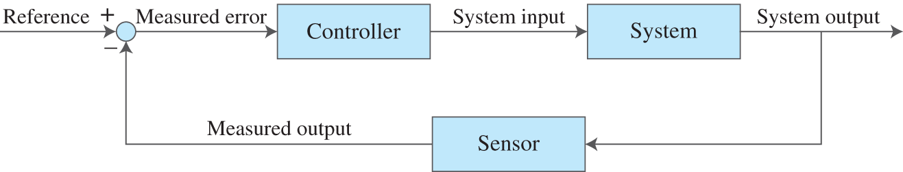
Figure 8.1 Typical block diagram of (negative) feedback control.
The theoretical basis of automatically controlling dynamical systems is the feedback loop [2]. Figure 8.1 presents its typical representation that consists of a reference signal that is compared with the measured output obtained by a sensor, which will lead to a measured error that will be used as the input of a controller that will act to modify the physical system, whose output is measured by the above‐mentioned sensor. The usual goal of the control mechanism is to minimize the difference between the reference signal (input) and the measured output. If the measured output is a trustworthy representation of the actual state of the physical system and the measured error tends to zero, then the mechanism designed to control the output of the physical system by a reference signal is successful.
Following the concepts introduced in the previous chapter, Figure 8.1 is a special case of a CPS, which is the scientific object of control theory [3] that has been supporting the technological development of a huge number of devices and tools, such as ovens, airplanes, power grids, and microelectronic circuits. However, our conceptualization is broader, and our study cannot be reduced to control theory despite the recent results in the field of networked control [4].
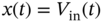
Before we move ahead, it is important to take a small step back and quickly overview the very basics of a field traditionally called Signals and Systems [5]. In its simplest form, continuous‐time signals are functions . For example, , where is the step function defined as if , and if . In this case, is a function of the continuous time . Figure 8.2 illustrates this signal.
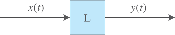
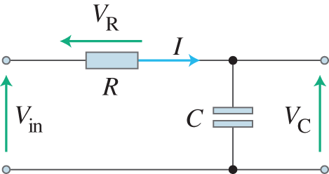
This signal can serve as an input of another element, usually denominated in the literature as a system (note that his definition of system is different from the one proposed in Chapter 2). Figure 8.3 presents a simple box diagram of the input–output relation caused by a given system. This abstraction represents actual physical relations that can be mathematically represented by operations like derivative, integration, and convolution with other signals. The resistor–capacitor (RC) circuit presented in Figure 8.4 is an example of a system that is mathematically characterized by the following equation
Figure 8.3 Schematic of a system whose input signal is and output signal .
Figure 8.4 RC circuit with an input signal and an output ; both are measured in volts. The system is defined by a connection between the resistor with the resistance and the capacitor with the capacitance .
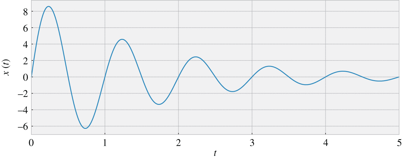
It important to reinforce that this relation is physical, and thus, the goal is to characterize the input–output relation by solving the differential equation. There are different possible ways to do it, but the method using Laplace or Fourier transforms is possibly the most commonly used one. The idea is to map the problem into another domain to then characterize the system by its response to an impulse signal, defining the transfer function of the system. This helps to solve the differential equation of linear and time invariant systems for an arbitrary input signal that has a well‐defined Laplace transform. Textbooks like [5] provide all the theoretical background, which is not our focus here, including an extensive analysis of definitions, properties, and classifications used in the field of signals and systems (with a special focus on the linear time‐invariant system). Figure 8.5 exemplifies the response that the RC gives to an input .
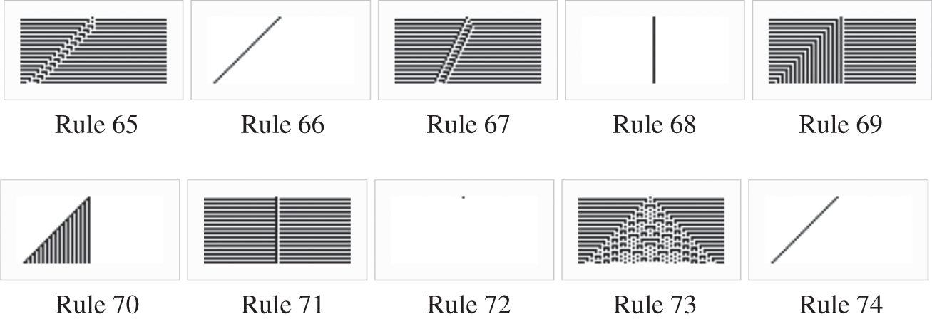
A similar conceptualization can be carried out for signals that are discrete in time, i.e. the time is indexed by a variable , forming an input sequence (or time series) and an output sequence . A discrete‐time version of the signal presented in Figure 8.2 is shown in Figure 8.6. The relation between input and output is given by difference equations, and the transfer function is obtained from a Z‐transform. The above‐mentioned book [5] also covers discrete‐time signals and systems.
Figure 8.5 Example of the input and output signals in the RC circuit presented in Figure 8.4 with k and nF. The input is a sequence of periodic pulses whose period is 0.1 second.
An important distinction worth mentioning is found between periodic and aperiodic discrete‐time signals, which is usually associated with event‐driven or event‐triggered approaches of data acquisition, signal processing, and control [6]. The idea behind this approach is to predefine events that will trigger the acquisition of a new sample or a control action. The events are generally defined through thresholds based on rules such as acquire a new sample if the measured signal is greater than a given value and act in the system if its measured output signal is below a given lower limit. These rule‐based behaviors are usually more complicated to be mathematically characterized (although possible in some cases), and therefore, computational models and heuristics are usually employed.
Another important classification relates to how many elements can take actions within the system boundaries, defining single‐agent and multiagent systems. The name multiagent system is quite informative because it is defined as a system composed of two or more elements that can internally take action capable of modifying its dynamics. The effects of each one of the agents and their combined actions in the system depend not only on the physical system itself but also on its structures of awareness and action, as indicated by the examples presented in the previous chapter. In the literature, multiagent systems are usually associated with collaborative control [7] by studying how the measurable attributes of the system are coupled (either via differential equations or computational models). There are a wide range of interesting examples, such as distributed control in power grids [8], swarm robotics [9], and random access in wireless networks [10].
Each case has its own very specific challenges, but all are CPSs following the approach taken in this book. In the next section, we will focus on one abstract example as a pedagogical tool to highlight the most relevant aspects of the dynamics of CPSs that are usually unclear when studying particular cases.
8.2 Dynamics of Cyber‐Physical Systems
As extensively discussed in Chapter 7, CPSs can be classified as a subclass of self‐developing reflexive–active systems constituted by three layers and cross‐layer processes. All CPSs then have the potential to change their internal states and their behavior following their self‐development, which may also include internal and external sources of uncertainty, and the relation to the environment as discussed in Chapter 2. A given system is usually classified by the characterization of the dynamics of some of its observable attributes, or metrics derived therefrom.
In this chapter, instead of focusing on any existing system, a simple – but extremely rich in its spatiotemporal dynamics – computational model called an elementary CA (see [1] will be employed as part of the data and decision layers of the CPS to be studied here. A brief description of such a model will be presented next.
(…) discrete, abstract computational systems that have proved useful both as general models of complexity and as more specific representations of non‐linear dynamics in a variety of scientific fields. Firstly, CA are (typically) spatially and temporally discrete: they are composed of a finite or denumerable set of homogenous, simple units, the atoms or cells. At each time unit, the cells instantiate one of a finite set of states. They evolve in parallel at discrete time steps, following state update functions or dynamical transition rules: the update of a cell state obtains by taking into account the states of cells in its local neighborhood (there are, therefore, no actions at a distance). Secondly, CA are abstract: they can be specified in purely mathematical terms and physical structures can implement them. Thirdly, CA are computational systems: they can compute functions and solve algorithmic problems.
Figure 8.7 Example of a two‐dimensional cellular automaton. Black cells are on, while state cells are off.
Figure 8.7 illustrates a snapshot of an example of a two‐dimensional CA where the cells can only assume two states, which are either on (black) or off (white).
A very simple class – which is called an elementary CA – is the one‐dimensional CA, where cells can be only on or off. The state of each cell depends on a given update rule that depends on the state of the cell itself and the state of its two neighbors, one on the right, the other on the left. Despite its simplicity, several interesting results can be derived from it so much so that Wolfram used it to claim the appearance of a New Kind of Science [1]. Without touching his extremely questionable position, Wolfram presents an extensive study of how the spatiotemporal development of the elementary CA may result in different patterns depending on the particular updating rule used by the cells. Before going into these details, we will present the fundamentals of the elementary CA.
Figure 8.8 exemplifies a typical development of an elementary CA, in this case using rule 30 and . Each row of the grid represents the state at a given discrete time , starting from . Hence, the two‐dimensional grid depicts the spatiotemporal development of the elementary CA. For rule 30 with the initial condition for and for , we can see an interesting pattern emerging over time.
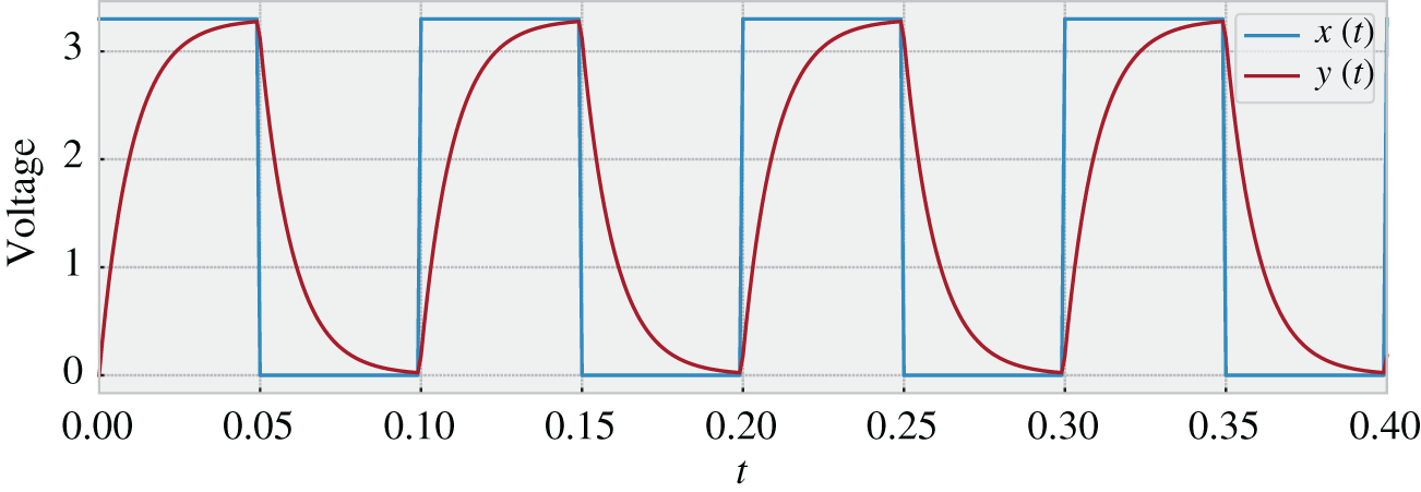
Different rules lead to different patterns, as indicated by Figure 8.9. Wolfram identified four different classes of patterns [pp. 231–235][1]:
In class 1, the behavior is very simple, and almost all initial conditions lead to exactly the same uniform final state.
Figure 8.8 Temporal development of an elementary CA with rule 30 for and initial states for and for , considering the border nodes and assuming that their missing neighbors are in state 0 (white).
In class 2, there are many different possible final states, but all of them consist just of a certain set of simple structures that either remain the same forever or repeat every few steps.
In class 3, the behavior is more complicated, and seems in many respects random, although triangles and other small‐scale structures are essentially always at some level seen.
(…), class 4 involves a mixture of order and randomness; localized structures are produced which on their own are fairly simple, but these structures move around and interact with each other in very complicated ways.
Of course, the development of the CA is deterministic given the set of initial conditions . The statistical analysis used by Wolfram to classify the spatiotemporal pattern generated by each rule, as well as other forms of classification, are beyond our scope here. The visual appeal is possibly the key here.
What is important for us is to know that the CA self‐development is associated with the updating rules and the initial conditions, whose spatiotemporal dynamics in the long run consists of:
a uniform pattern (class 1);
a periodic pattern (class 2);
chaotic (aperiodic) patterns (class 3);
complex patterns with localized structures (class 4).
In the next section, we will study how the elementary CA could serve to represent the data and decision layers of a CPS.
8.2.2 Example of a Cyber‐Physical System
Consider a CPS in which the physical layer is the electric circuit presented in Figure 8.10. There is a constant voltage source associated with a resistor that supplies electric power to pairs of resistors in parallel, which may represent a toy model of microgrids [12]. Each pair has one resistor that is always active (i.e. a base load) and another that may be connected or not depending on the state on () or off () of its associated switch (i.e. flexible load).
If we assume that and that the number of resistors in the on state is , then we can compute the equivalent resistor of the circuit as
(8.1)
The extreme cases are then when all the flexible loads are connected, and we have thus and none . If different discrete observation times are considered, then we have , and .
Now, this circuit is the physical layer of CPS that is a discrete‐time self‐developing system where its data and decision layers are constructed upon the elementary CA with elements. Each element is both a decision‐maker that follows the updating rule defined by the CA and an agent to connect or disconnect the flexible load accordingly. We can then define as follows.
Input: in volts, and output: in watts where the equivalent resistor in ohms depends on the number of how many elements are states (on or off) at discrete‐time .
SAw:. This indicates that all elements receive data directly from the physical layer. Besides, the level 2 processes indicate that to make a decision, the element has an image of its own state as well as of its direct neighbors and , also considering that the border elements have only one neighbor.
SAc:. This indicates that elements are agents that directly act on their own switches.
Figure 8.10 Example of an electric circuit with agents.
Remember that the SAw tells nothing about the trustworthiness of the data. Additionally, in this specific case, the SAw and SAc are fixed over time.
Figure 8.11 presents the outcome of the CPS whose input is and the output is for a given where represents a specific discrete time index; the resistors are arbitrarily chosen as m and . This figure presents the dissipated power considering different numbers of active flexible loads, which are directly obtained from the state of the CA in time . It is important to note that we are analyzing this CPS as a “black box” where, for a given input , we can only observe the total dissipated power as the output of the discrete time . The relation between the CPS internal dynamics and the observable outcomes will be presented next.
8.2.3 Observable Attributes and Performance Metrics
As indicated in the previous section, the only attribute of the system that can be observed by an external element is the dissipated power at time by the CPS for a given input voltage . If the observable variable is trustworthy, then it is possible to unambiguously determine the number of flexible loads that are active in time . However, the sequences and could potentially be the outcome of different rules of the elementary CA.
Figure 8.11 Numerical example of the CPS for m and . The input is in volts and the output is the total power in watts dissipated in time considering different numbers of active flexible loads.
Depending on the CPS requirements, even though a given outcome might be acceptable, it may also be produced by an internally undesirable dynamics. For example, a similar behavior might be produced by a fair activity allocation. This can be measured by a simple performance metric that computes the ratio between how many times a given agent was in an active state, i.e. , and the time window under consideration. Mathematically, we have , considering an arbitrary time window of starting at and ending at . At the system level, another performance metric could be the ratio between the number of agents in the active state divided by the number of agents .
Figure 8.12 illustrates the dynamics of CPS for two different update rules, namely 54 and 73, with a total of flexible loads controlled by their respective agents. The physical layer setting is m and . The input is V (fixed) and the output is the observable sequence , whose values depend on the initial states and the aforementioned update rules. For this experiment, a random initial state is considered where each state with is randomly chosen following an independent and identically distributed random variable where and . We set the same initial states for both cases, and the difference in their dynamics is only due to the decision rules based on the CA. We study a time window starting from and ending in .
Figure 8.12 Dynamics of CPS for rules 54 and 73 considering V, m, and . (a) Sequence (observable variable) for rule 54. (b) Sequence (observable variable) for rule 73. (c) CA development for rule 54. (d) CA development for rule 73. (e) Ratio for rule 54. (f) Ratio for rule 73. (g) Ratio considering agent for rule 54. (h) Ratio considering agent for rule 73.
There are interesting things to note in this illustrative scenario, which we will list below.
Figure 8.12a, b indicate that the two CPSs lead to sequences with a similar mean value of dissipated power (approximately 150 W) and a similar behavior, although the first case presents more oscillations.
Rules 54 and 73 have different classes as presented in Figure 8.12c and d, respectively. Rule 54 is class 4 (complex patterns, visually identified by the triangles of different sizes), while rule 73 is class 2 (periodic behavior).
The ratio of active flexible loads in the physical layer is also similar, around 50%, as shown in Figure 8.12e and f (although the first varies more). This is true for both rules regardless of the initial condition being .
Figure 8.12g, h show a remarkable difference of fairness related to the different agents (and their flexible loads). The first case (rule 54) has the largest majority of its flexible loads active with a similar ratio (i.e. activity frequency is around 1‐out‐of‐2). The second case (rule 73) has a very large variation: several flexible loads almost never active , others almost always active , others with , and still a few others with different ratios.
What is remarkable is that both CPSs have a similar observable outcome that is the result of very different internal dynamics. This fact is not always true because different rules may lead to different observable outcomes, as it may be inferred from Figure 8.9. Besides, some rules may be more sensitive to different initial conditions. These aspects will be presented in the next section when we aim to optimize the CPS dynamical behavior.
8.2.4 Optimization
Optimization as described in Chapter 6 is associated with the determination of operational points or system parameters that maximize or minimize a given performance metric subject to a set of constraints. The proposed CPS is an example of a self‐developing system such that an optimization would in principle be unfeasible. To formulate a proper optimization problem, we first need to specify its desirable operational outcomes, internal constraints, and design parameters. These specifications are given below.
The operational objective is to guarantee that is within the range determined by the upper and lower limits of dissipated power.
All flexible loads should be active with a similar frequency.
The parameters of the physical layer are given and fixed, as well as the SAw and the SAc.
The only design parameter is the update rule of the elementary CA.
The initial conditions are unknown.
In this case, the optimization problem could be formulated in two different ways as follows:
select the rule that minimizes the frequency thatis out of its operational range subject to a fair activity frequency among the flexible loads, or
select the rule that maximizes the fairness of activity frequency among the flexible loads subject towithin its operational range.
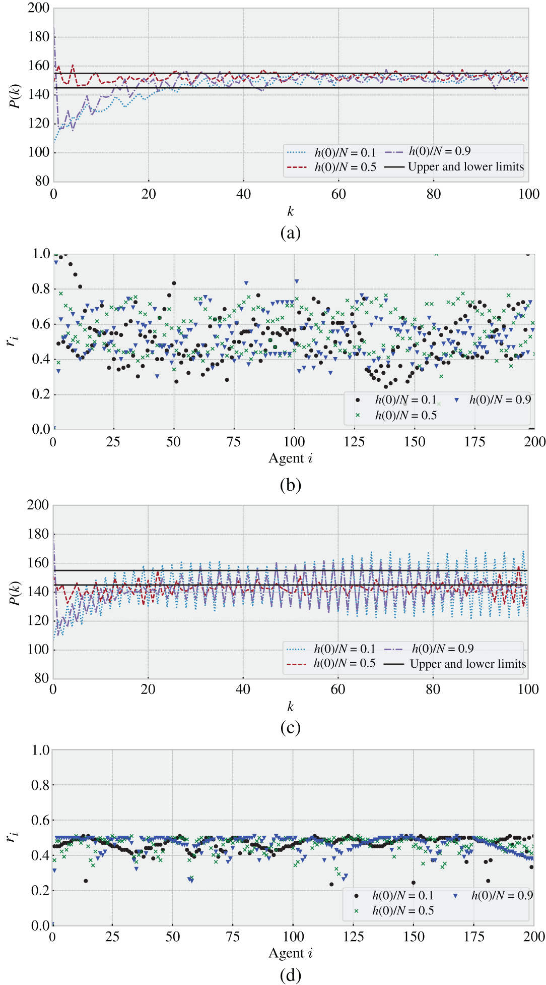
Although it would be possible to write it both in mathematical terms and possibly solve it at least for special cases, we rather prefer typical outcomes considering different update rules and random initial conditions. Such a numerical analysis is presented in Figure 8.13, where the dynamics of the dissipated power is depicted considering rules 81, 82, 84, 110, 240, and 250 for three different initial conditions, and V, m, and . By inspection, rule 110 seems a suitable rule because it is the only one that is consistently within the operational range. It is interesting to note that rule 110 tends to move quickly to the desired range regardless of the initial condition, while the other rules seem to have either different “attractors” or an oscillatory behavior heavily dependent on the initial conditions.
However, this figure does not indicate the fairness in the flexible load activity in the system. Figure 8.14 presents the performance of rule 110 by showing the dynamics over time for three different initial conditions together with the allocation fairness evaluated by the ratio . Besides, Figure 8.14 also shows the same plots for rule 54, which presented a reasonable performance as indicated by Figure 8.12. Figure 14a confirms that the CPS mostly work within its operational limits. However, Figure 8.14b shows that the fairness of the system it not so high, regardless of the initial condition, because the ratios are quite dispersed (but not as much as in the situation presented in Figure 8.12h). On the other hand, Figures 8.14c and d present a different behavior: a stronger dependence on the initial conditions and a fair activity frequency of flexible loads. It is also interesting to see that, although being always around the operational limits, the CPS rarely operates with the desired range. An interesting note is that both rules 110 and 54 are class 4.
Considering all the rules studied in this section, we infer that rule 110 would be the optimal solution among the options presented here. It seems to provide a system whose internal dynamics will tend to a sequence that operates almost always within the required range regardless of the initial conditions, while the different flexible loads have a reasonably fair distribution. However, this is just an indication, and there might be another rule that provides better outcomes. It would also be interesting to prove mathematically the insights provided by these numerical examples. One remarkable thing is that different classes of rule may have the same observable outcomes but produced by a quite different internal dynamic. These results, however, considered an ideal scenario without any failure or intentional attacks against the CPS , which is the topic of the following section.
Figure 8.13 Dynamics of CPS for different rules and initial conditions considering V, m, and . (a) Sequence (observable variable) for the initial condition uniformly distributed so that and . (b) Sequence (observable variable) for the initial condition uniformly distributed so that and . (c) CA development for initial condition uniformly distributed so that and .
8.3 Failures and Layer‐Based Attacks
In comparison with physical systems, CPSs have an increased vulnerability. The constitution of CPSs in three layers opens new possibilities of failures related to the cyber domain. For example, the data acquired by sensors might be noisy, or communication links might be subject to errors. These types of issues may lead to misinformation (unintentional) or disinformation (intentional), as defined in Chapter 4. Regardless of their nature, untrustworthy data may result in decisions and then actions that would modify the dynamics of the CPS potentially affecting all three layers. Throughout this section, we will analyze the impact of failures and attacks based on the already discussed CPS .
At the physical layer, failures or attacks are related to the electric circuit depicted in Figure 8.10 itself. A wire or cable could be (intentionally or not) broken, disconnecting some elements of the system or even the whole system. There are other possibilities: the input could be (intentionally or not) modified or the switches could be (intentionally or not) broken. In all those cases, the changes in the system dynamics are captured by the mathematical equations.
These modifications, however, do not necessarily alter the acquired data to be used in the cyber domain. For instance, depending on how data are acquired, a broken switch may not act as expected by the decision‐making element, and thus, the state of the agent might be different from the actual physical situation. If this is the case, the data will be unrelated to the actual physical state, and thus, the outcome of the CPS will be affected. Besides, this effect also propagates because of the SAw that requires communication between the agents, which also use the problematic data as part of their on decision‐making process. The communication between the agents might also be a source of failures in the CPS operation.
Figure 8.15 exemplifies a misinformation cyberattack where the communication link from Agent 99 and Agent 100 is actively attacked by injecting a misinformation of the state of the former, namely , to modify the decisions of the latter, affecting then the dynamics of the CPS. By comparing Figure 8.15a–c, it is easy to verify the impact of the cyberattack and its dependence on the fake state, either in Figure 8.15b or in Figure 8.15c. Figure 8.15d demonstrates the physical effect of the injection of fake data, modifying the temporal development of the CPS, which is reflected by the change of the observable sequence for . The activity ratio is also affected by the misinformation attack. In this specific case governed by rule 245, the changes only affect the elements on the right side of the attacked one, reaching one more element at each discrete time.
Figure 8.14 Dynamics of CPS for different rules 110 and 54 considering V, m, and , and different initial conditions. (a) Sequence for rule 110. (b) Ratio considering agent for rule 110. (c) Sequence for rule 54. (d) Ratio considering agent for rule 54.
Figure 8.15 Dynamics of CPS for rule 254 considering V, m, and for the initial condition uniformly distributed so that and . A cyberattack is injected at the communication link from agent 99 to 100 staring at time so that the latter will always receive a fake state . (a) CA development for rule 245 in normal operation. (b) CA development for rule 245 with a cyberattack . (c) CA development for rule 245 with a cyberattack . (d) Sequence for rule 245 with and without a cyberattack. (e) Ratio considering agent for rule 245.
The same procedure could be performed with other rules and other physical layers, and thus, other particular results will be found. What is important to keep in mind is that the three layers are constitutive of CPSs, and thus, all the three layers are vulnerable to attacks. A simple cyberattack may indirectly affect the dynamics of observable physical variables without any foreseeable justification.
8.4 Summary
This chapter introduced important ideas related to the dynamics of CPSs following the three‐layer approach. Our aim here was to provide an intuitive while theoretically sound example of a CPS whose data and decision layers are defined by the elementary CA, well known for its four classes of spatiotemporal classes of behavior [1]. We have also shown how the system dynamics based on observable variables might hide an intricate internal dynamic. In addition, a new cyber domain enables different sources of failure points and vulnerabilities compared with purely physical systems. Although linked to the theme of this chapter, topics related to established disciplines like systems and signals [5] and control theory [3, 4] were not covered, and the readers are suggested to refer to them by incorporating the theory of CPS presented here. The book [14] focuses on different aspects of the combination of control theory and computer sciences to design CPSs, which can be seen in many ways complementary to the approach focusing on a representative but purified model taken by this chapter. In the next part of this book, we will move from the abstract theory proposed in parts 1 and 2 to then return to aspects concerning the material world, including examples of CPSs, the enabling information and communication technologies, and social impact.
Exercises
8.1CPS dynamics Consider the CPS analyzed in Sections 8.2 and 8.3. Study four different rules following the examples provided in that section, repeating the results from Figures 8.12 to 8.15. Analyze the results. The code is available at https://github.com/pedrohjn.
8.2Impact of defining initial conditions Consider the same CPS as the one studied in Exercise 8.1. The aim of this task is to analyze the impact of defining the initial conditions of the elements. Find a combination of an initial condition and rule that provides the desirable outcome based on the specification given in Figure 8.14. Hint: Find the desired dynamics of the sequence , and then, write the truth table as presented in Table 8.1 to find the desired rule.
References
1 Wolfram S. A New Kind of Science. vol. 5. Wolfram Media, Champaign, IL; 2002.
2 Wiener N. Cybernetics or Control and Communication in the Animal and the Machine. MIT Press; 2019.
3 Lewis FL. Applied Optimal Control and Estimation. Prentice Hall PTR; 1992.
4 Zhang XM, Han QL, Ge X, Ding D, Ding L, Yue D, et al. Networked control systems: a survey of trends and techniques. IEEE/CAA Journal of Automatica Sinica. 2019;7(1):1–17.
6 Miskowicz M. Event‐Based Control and Signal Processing. CRC Press; 2018.
7 Lewis FL, Zhang H, Hengster‐Movric K, Das A. Cooperative Control of Multi‐Agent Systems: Optimal and Adaptive Design Approaches. Springer Science & Business Media; 2013.
8 Sahoo S, Mishra S, Jha S, Singh B. A cooperative adaptive droop based energy management and optimal voltage regulation scheme for DC microgrids. IEEE Transactions on Industrial Electronics. 2019;67(4):2894–2904.
9 Rinner B, Bettstetter C, Hellwagner H, Weiss S. Multidrone systems: more than the sum of the parts. Computer. 2021;54(5):34–43.
10 Popovski P. Wireless Connectivity: An Intuitive and Fundamental Guide. John Wiley & Sons; 2020.
12 Kühnlenz F, Nardelli PHJ, Alves H. Demand control management in microgrids: the impact of different policies and communication network topologies. IEEE Systems Journal. 2018;12(4):3577–3584.
13 Kühnlenz F, Nardelli PHJ. Dynamics of complex systems built as coupled physical, communication and decision layers. PLoS One. 2016;11(1):e0145135.
14 Alur R. Principles of Cyber‐Physical Systems. MIT Press; 2015.

 .
.
 whose input signal is
  and output signal
  .
.
 and an output
 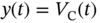 ; both are measured in volts. The system is defined by a connection between the resistor with the resistance
  and the capacitor with the capacitance
  .
.
 k
k and
and  nF. The input is a sequence of periodic pulses whose period is 0.1 second.
![Schematic illustration of example of a discrete-time signal x[k].](https://imgdetail.ebookreading.net/2023/10/9781119785163/9781119785163__9781119785163__files__images__c08f006.png)
 .
.
![Schematic illustration of temporal development of an elementary CA with rule 30 for N=31 and initial states si[0]=0 for i≠15 and si[0]=1 for i=15, considering the border nodes i=1 and i=31 assuming that their missing neighbors are in state 0 (white).](https://imgdetail.ebookreading.net/2023/10/9781119785163/9781119785163__9781119785163__files__images__c08f008.png)
and initial states
for
and
for
, considering the border nodes
and
assuming that their missing neighbors are in state 0 (white).
 in volts, and output:
 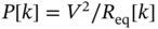 in watts where the equivalent resistor
  in ohms depends on the number
  of how many elements are states (on or off) at discrete‐time
  .
. . This indicates that all elements receive data directly from the physical layer. Besides, the level 2 processes indicate that to make a decision, the element
  has an image of its own state as well as of its direct neighbors
  and
and  , also considering that the border elements have only one neighbor.
 . This indicates that elements
  are agents that directly act on their own switches.
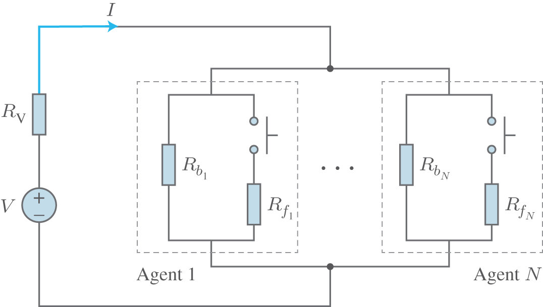
 agents.
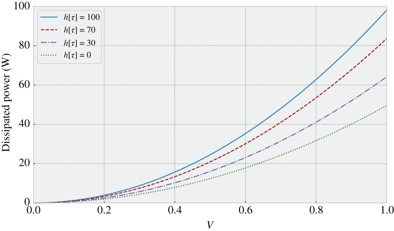
 for
for  m
m and
and  . The input is
  in volts and the output is the total power
  in watts dissipated in time
  considering different numbers
  of active flexible loads.
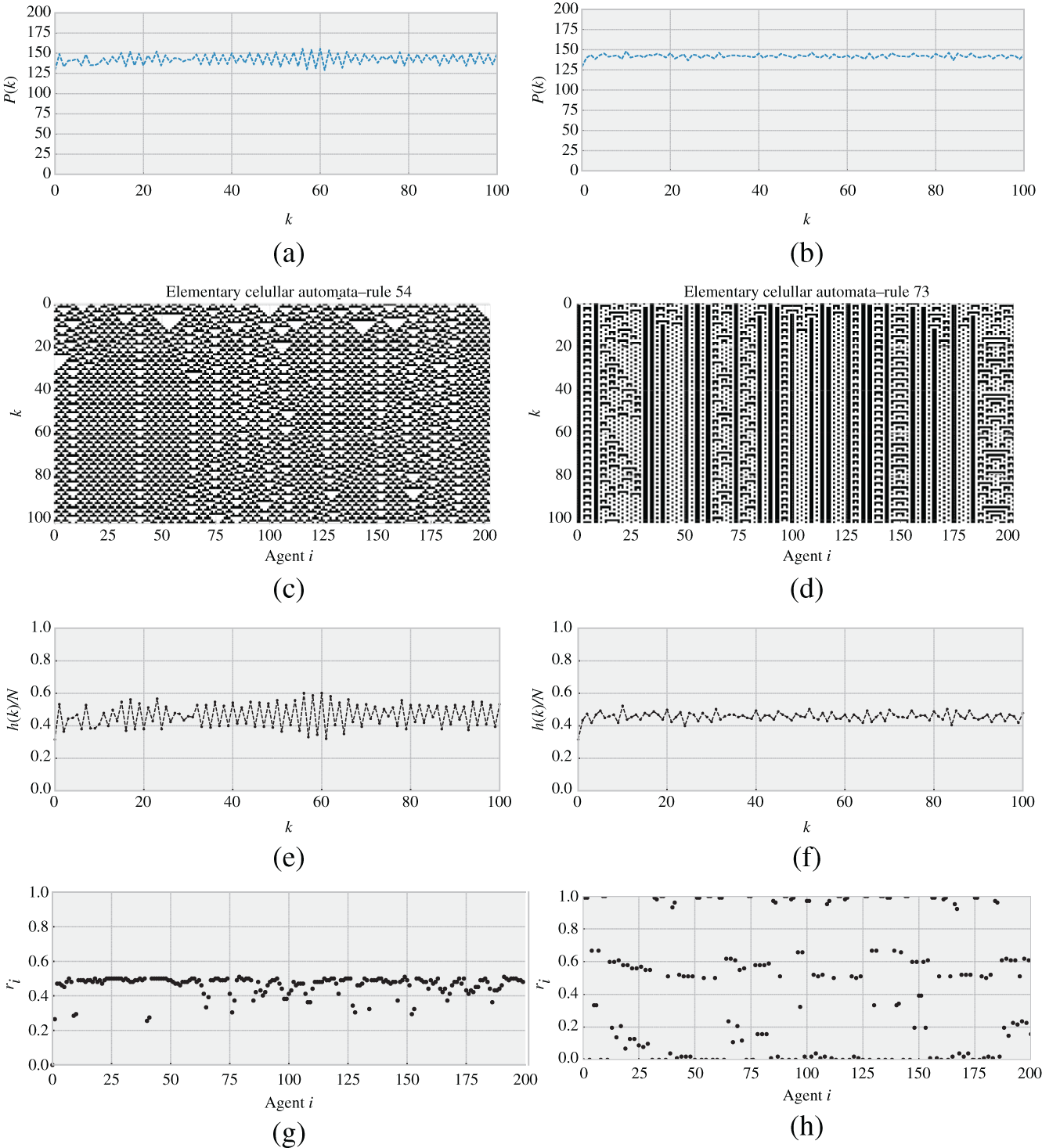
 for rules 54 and 73 considering
  V,
V,  m
m , and
, and 
 . (a) Sequence
  (observable variable) for rule 54. (b) Sequence
  (observable variable) for rule 73. (c) CA development for rule 54. (d) CA development for rule 73. (e) Ratio
  for rule 54. (f) Ratio
  for rule 73. (g) Ratio
  considering agent
  for rule 54. (h) Ratio
  considering agent
  for rule 73.
 with a similar mean value of dissipated power (approximately 150 W) and a similar behavior, although the first case presents more oscillations.
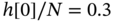 .
. (i.e. activity frequency is around 1‐out‐of‐2). The second case (rule 73) has a very large variation: several flexible loads almost never active
  , others almost always active
  , others with
  , and still a few others with different ratios.
 is within the range determined by the upper and lower limits of dissipated power.
 is out of its operational range subject to a fair activity frequency among the flexible loads, or
 within its operational range.
 for different rules and initial conditions considering
  V,
V,  m
m , and
, and 
 . (a) Sequence
  (observable variable) for the initial condition uniformly distributed so that
  and
and  . (b) Sequence
  (observable variable) for the initial condition uniformly distributed so that
 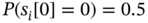 and
and 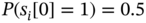 . (c) CA development for initial condition uniformly distributed so that
  and
and  .
.
 for different rules 110 and 54 considering
  V,
V,  m
m , and
, and 
 , and different initial conditions. (a) Sequence
  for rule 110. (b) Ratio
  considering agent
 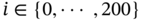 for rule 110. (c) Sequence
  for rule 54. (d) Ratio
  considering agent
  for rule 54.
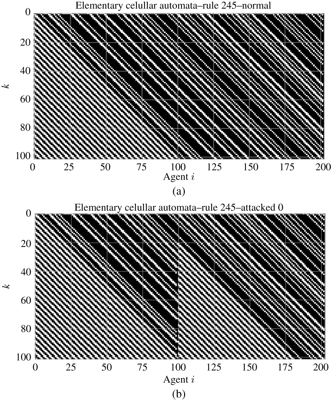
 for rule 254 considering
  V,
V,  m
m , and
, and 
 for the initial condition uniformly distributed so that
  and
and  . A cyberattack is injected at the communication link from agent 99 to 100 staring at time
  so that the latter will always receive a fake state
  . (a) CA development for rule 245 in normal operation. (b) CA development for rule 245 with a cyberattack
  . (c) CA development for rule 245 with a cyberattack
  . (d) Sequence
  for rule 245 with and without a cyberattack. (e) Ratio
  considering agent
  for rule 245.
 , and then, write the truth table as presented in Table 8.1 to find the desired rule.