
Appendix A
General Cost of Delay Formula
Cost of Delay can be calculated in the case where the cumulative income curves can be represented as functions of time.
Consider the cumulative income curves of Investments 1–3 represented by f1(t), f2(t), f3(t) with cycle times T1, T2, T3, respectively, where f1(t) = 15t, f2(t) = 10t1.5, and f3(t) = 8t1.8. Time units are in quarters, income in $K. Figure A.1 shows the development order f1(t), f2(t), f3(t).
f2(t) is delayed by T1 while Investment 1 is developed. The deferred income from f2(t) is what would have been produced by f2(t) when the first Investment was completed, which is f2(T1). f3(t) is delayed by T1 + T2 by the development of Investments 1 and 2. By time T2 Investment 3 could have generated f3(T1 + T2). The order f1(t), f2(t), f3(t) produces the lowest Net Cost of Delay if f2(T1) + f3(T1 + T2) is the minimum for all permutations of f1(t), f2(t), f3(t) .
This requires computation of Net CoD for values for the permutations as shown in Table A.1.
Net Cost of Delay for each combination is calculated in Table A.2.
The order f1, f3, f2 has the lowest Net Cost of Delay in this example.
The calculations can be completed for any set of Investments. However, the number of calculations is N! where N is the number of Investments. There are 120 permutations for five Investments and increases to over 3 million for 10 permutations.
There is an inherent assumption that the order of Investment development does not impact cycle time. This is true for interchangeable resources but not when development must wait for specific skills. For example, there could be limited database or backend developers to support all the Investments. This requires a more complex algorithm where cycle times are based on availability of critical path skills.
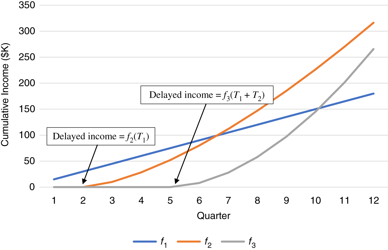
Figure A.1 Cumulative income based on project order.
Table A.1 Net Cost of Delay formulas for three Investments.
| Order | Net Cost of Delay |
|---|---|
| f1(t), f2(t), f3(t) | f2(T1) + f3(T1 + T2) |
| f1(t), f3(t), f2(t) | f3(T1) + f2(T1 + T3) |
| f2(t), f1(t), f3(t) | f1(T2) + f3(T2 + T1) |
| f2(t), f3(t), f1(t) | f3(T2) + f1(T2 + T3) |
| f3(t), f1(t), f2(t) | f1(T3) + f2(T3 + T1) |
| f3(t), f2(t), f1(t) | f2(T3) + f1(T3 + T2) |
Table A.2 Net Cost of Delay calculation example for three Investments.
| Order | Net CoD ($K) |
|---|---|
| f1, f2, f3 | 230 |
| f1, f3, f2 | 175 |
| f2, f1, f3 | 261 |
| f2, f3, f1 | 247 |
| f3, f1, f2 | 316 |
| f3, f2, f1 | 297 |
A.1. Reinertsen WSJF
The general Cost of Delay formula is another way to prove Reinertsen's Weighted Shortest Job First (WSJF) formula. Consider two Investments (or projects) with Costs of Delay C1 and C2. If Investment 1 is developed first, the Net Cost of Delay for Investment 2 is f2(T1). For the opposite order, the Net Cost of Delay is f1(T2).
Investment 1 should be prioritized if
or

Unfortunately, the cross‐multiplication only works for the linear case of income generated at a constant rate. Otherwise, a calculation table as shown in the example must be generated for all Investment combinations.
A.2. Income Curve Approximation
There are two options for determining the cumulative income profile function based on quarterly cumulative income projections. The first is to fit the curve to a power function of the form.
This can be done with the Excel LINEST linear regression formula. Taking the logarithm of both sides of the formula gives:
Consider the projected cumulative income example shown in Table A.3.
The logarithms of the x and y variables are shown in Table A.4.
The Excel LINEST linear regression can be used to estimate the slope and y‐intercept.
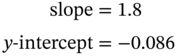
Table A.3 Cumulative income example.
| Quarter | Cumulative income ($K) |
|---|---|
| 1 | 1 |
| 2 | 3 |
| 3 | 5 |
| 4 | 10 |
| 5 | 14 |
| 6 | 16 |
| 7 | 20 |
| 8 | 36 |
| 9 | 45 |
| 10 | 60 |
| 11 | 70 |
| 12 | 90 |
Table A.4 Logarithms of quarter and cumulative income.
| Log (Quarter) | Log (Cumulative income) |
|---|---|
| 0.0 | 0.0 |
| 0.3 | 0.5 |
| 0.5 | 0.7 |
| 0.6 | 1.0 |
| 0.7 | 1.1 |
| 0.8 | 1.2 |
| 0.8 | 1.3 |
| 0.9 | 1.6 |
| 1.0 | 1.7 |
| 1.0 | 1.8 |
| 1.0 | 1.8 |
| 1.1 | 2.0 |
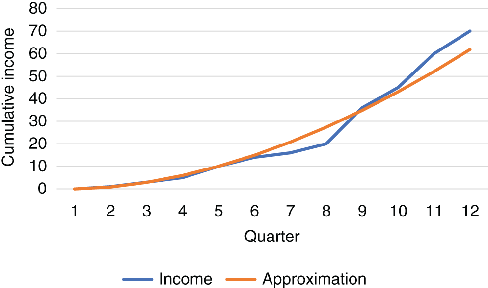
Figure A.2 Income profile nonlinear regression.
The y‐intercept is log(a) so:
The best fit for the income ramp is:
Figure A.2 shows that this formula provides a close fit for cumulative income, certainly well within the income estimation variance.
Separate log and linear regression Excel functions were used for this example to illustrate the method. There is also an Excel LOGEST function that may be used to directly calculate the coefficient and exponent.
The “logistics curve” can also be used to estimate annual income, known as the “S‐curve” given by:
- L = maximum value
- k = slope of the curve at the inflection point, also called “the logistics growth rate”
- T0 = the time value at the inflection point
The curve is often used to describe physical phenomena like population growth where growth increases gradually at first, more rapidly in the middle growth period, leveling off as saturation occurs. It can be used to model deployment of software upgrades.
A.3. Summary
- Net Cost of Delay can be calculated for income curves that can be represented as a function of time, but complexity of the calculation increases significantly with the number of Investments. The formula has been included for completeness; but in most cases, the rate at which income is shifted out of a three‐year planning period will suffice for the Cost of Delay calculation because most large companies are more concerned with near‐term income predictability.
- The general formula reduces to Reinertsen's WSJF for the case of linear income ramps.
- Most cumulative income ramps can be estimated by fitting a power curve to quarterly forecasts or using the logistics formula.