
8
Releasing Investments
Competition for R&D capacity based on Weighted Shortest Job First (WSJF) creates incentives to plan and build smaller Investments. Planning does not begin with a release assumption in the Investment model. Income generation for bundled Investments is delayed until the release date. The first objective is to plan Investments that can be released independently. However, there are instances where Investments will need to be bundled within releases.
This chapter begins with new insights into the opportunity cost of bundled releases based on Net Cost of Delay. Quantifiable Cost of Delay allows us to calculate the income lost by delaying a completed Investment to the release date. Release trains cost the software industry billions of dollars that are invisible today. WSJF changes the economics of release planning by showing how overall R&D Return on Investment (ROI) can be increased by investing in architectural and other technical changes to simplify deployment for the organization and its customers. Many engineering organizations know how they can simplify deployment but can't justify the development costs. Organizations can now see the “opportunity cost of not being Agile.” Millions of dollars are being “left on the table,” some of which can be recovered with software infrastructure changes to reduce deployment time.
We examine the reasons why large releases persist despite the industry transition to Agile development. We also address why many customers won't accept releases more frequently even if a company can reduce development cycle time, and how to overcome their reluctance.
Lastly, another form of Work in Process (WIP) will be discussed that has not been considered in software development. A manufacturing analogy of inventory cost management is used to reveal the cost of capital tied up in a release, providing another financial justification for releasing Investments independently.
8.1 Release Opportunity Cost
Continuous Delivery (CD) is the dream of every software company. Income can be generated as soon as an increment of business value is developed. Customers like CD because they receive value from software sooner and don't experience the effort and risk of large releases. However, CD is not widespread in the software industry, especially in larger organizations that have traditionally delivered periodic releases.
Most of the CD examples I've seen are in Business‐to‐Consumer (B–C) companies. Updating a website is a typical example. Another example is Google updating their search algorithm on a daily or weekly basis. Business‐to‐Business (B–B) companies often deliver upgrades that involve significant customer effort and changes to the way they work. Some regulated industries, like life sciences, require comprehensive validation testing after each upgrade, placing further burden on the customer. There will be cases where Investments need to be bundled into a release, but they should be justified as exceptions.
Part of the problem is that software companies have been unaware of the opportunity cost of releases. Figure 8.1 demonstrates the financial value of reducing release cycle time.
The solid line in the chart (Figure 8.1) shows cumulative income for annual releases with a Cost of Delay of $1M per month. There is no income in the first year while the first release is under development. After the first year, income of $1M per month is generated. The second release starts contributing an additional $1M per month after the second year for a total of $2M per month. The solid line shows that cumulative income reaches $36M at the end of the second year for the annual release case.

Figure 8.1 Cumulative income by relative cycle time reduction.
The line with small dots assumes that each annual release can be split in half, each release generating half the monthly income. Since the release value is halved, the Cost of Delay is reduced from $1M per month to $0.5M per month. Income begins to flow after six months, with $0.5M per month added every six months thereafter, for a total of $45M at the end of the second year. The other lines show how the income increases within the same period based on shorter release cycles. A factor of 12 for the monthly case generates $52.5M in the same period.
Consider the question, “What software development productivity improvement would I need to achieve to increase income from the annual release total of $36M for the annual release case to $53.5M generated by the monthly release case?” Total productivity is Value Out/Value In. Assume the development costs are the same for both cases (release overhead costs are addressed later in the chapter). Productivity would have to increase by a factor of 52.5/36 = 1.46, a 46% improvement.
Table 8.1 shows the income accumulated over the three‐year period for each release cycle time reduction, with an increase in total productivity over the three‐year period relative to the annual release case.
The first observation is that reducing release cycle time can substantially improve total productivity. The second observation is that the benefits of reduced release cycle times have diminishing value. Total productivity is improved by 25% going from annual to semiannual releases. Moving from monthly to quarterly releases relative to annual releases improves productivity only by (52.5 − 49.5)/49.5 = 6%.
Appendix B provides a general formula that relates the fractional reduction in cycle time to equivalent total productivity improvement. Assume N is the fractional reduction in cycle time. For example, N = 2 for the case of moving from annual to semiannual releases. N = 4 for annual to quarterly releases. Appendix C derives a formula for productivity improvement as a function of release cycle reduction. The ratio of total productivity is determined by
Table 8.1 Equivalent productivity improvement as a function of release frequency.
| Release cycle (Annual to) | Income ($M) | Productivity increase relative to annual releases (%) | Point difference from the release case above |
|---|---|---|---|
| Annual | 36 | — | — |
| Semiannual | 45 | 25 | 25 |
| Quarterly | 49.5 | 37.5 | 12.5 |
| Monthly | 52.5 | 46 | 8.5 |

Figure 8.2 Total equivalent productivity improvement for release cycle time improvement.
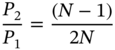
Figure 8.2 plots the equivalent productivity improvement for fractional reductions up to 12, equivalent to moving from annual releases to monthly releases.
Moving to CD is like splitting the release into an infinite number of release segments, each with infinitely small value. The limit of the productivity formula is 50%. The point difference between the monthly and the ideal CD release cases is only 4%.
The analysis shows that companies are losing millions of dollars today from the inability to reduce release cycle times. Money spent to reduce cycle times can provide a positive ROI.
8.2 Investment Release Bundling
Although every attempt is made to plan and develop deployable Investments, there will be times when they will need to be bundled into a release. There are three reasons for Investment bundling:
- Investments can't be priced independently.
- Customers reject more frequent releases.
- Investment deployment overhead costs.
8.2.1 Investment Pricing
Many organizations have established an upgrade pricing model for their customers. Customers are charged an upgrade fee plus monthly or annual support and maintenance fees. Customers often budget based on annual upgrades. Pricing independent Investments may be a challenge in this case because it changes the customer's budgeting model; therefore, Investments may have to be bundled into releases.
Software as a Service (SaaS) has become a popular pricing model. Customers pay on a periodic basis, often monthly. Quite often, the price includes future upgrades. Features are added to releases to maintain and attract customers to grow revenue but organizations do not increase the price for individual customers. In this case, the advantage of releasing Investments independently is diminished because the income impact is based on market growth. For example, a difference of three months in Investment release dates may not justify the additional overhead costs of separate releases.
The Investment model lends itself to value‐based pricing. There are several pricing models for SaaS pricing, such as user‐based and tier‐based pricing. The objective of each model is to relate pricing to the value the customer receives from the product. This book will not go into the many SaaS pricing options available. We will focus on a model in which customers are willing to pay more based on the additional value they receive from an Investment.
This brings up the opportunity for modular pricing, where Investments can be selectively purchased by customers. Pricing is based on the value the customer receives. Deploying independent Investments is more important in modular pricing because there is an immediate impact on income generation. Modular pricing should be the objective of companies that adopt the Investment model. It can substantially increase near‐term income, providing lower payback periods at reduced risk.
The top line in Figure 8.3 represents lifetime deployment of a typical product. Growth is slow to start and then accelerates quickly as product adoption increases. Sales start to drop as the product approaches the point of market saturation. New sales diminish as the market becomes saturated. Cumulative installations follow the classic S‐curve. Most companies continue to build large releases for initial installation without considering upgrades as a separate market segment.
The Net Cost of Delay depends on the rate at which customers accept modular Investments. This can be high if the customer perceives value to justify the Investment and if upgrades are seamless. Investments can provide a vehicle for planning modular upgrades of tangible value. Modular pricing for your installed base market segment can result in reduced payback periods because customers have already been acquired.

Figure 8.3 Typical product life cycle.
8.2.2 Lack of Customer Acceptance
Customer acceptance often comes up in customer discussions on reducing cycle time. “Even if we could release faster, our customers wouldn't accept more frequent releases.” This may be true, but you need to think about why that is the case. Certainly, customers want to obtain value from your software as often as possible. Somehow, the customer burden of upgrading your software outweighs perceived value. This must be overcome if you are to attain the full benefits of the Investment model.
In many cases, customers have experienced upgrade quality problems that significantly impacted their operations. The potential risks outweigh any perceived benefits. High quality is a prerequisite for releasing faster. It is a difficult challenge, but software upgrades must be virtually defect‐free. Don't expect your customers to accept releases more frequently if they risk disruption to operations.
Unfortunately, there is no “magic bullet” for reaching near zero‐defect code quality. It requires sound software engineering quality practices. The quality bar cannot be lowered for Agile development. Even though Agile uses shorter development cycle iterations, good software engineering practices must apply, such as code reviews and automated unit regression tests with adequate coverage.
Agile development has the potential to produce higher‐quality software than Waterfall does. The short development iterations can provide rapid quality feedback during release development. Retrospectives facilitate process improvement throughout the development cycle. Maintaining software in a “potentially shippable” state reduces rework and the side effects of fixes late in the release development cycle. However, in many of the organizations I've assessed, the minimalist “Agile” philosophy is believed to apply to software engineering practices. The same Waterfall quality software engineering practices need to be in place. Accept that reducing cycle time is likely to have little benefit if you can't deliver near defect‐free software. Chapter 12 addresses software quality.
Feature‐based planning presents a significant obstacle to reducing cycle time. Large releases today are stuffed with feature requests from multiple customers. Product managers “sprinkle” features in releases to try to quell demands. Quite often, this results in releases that contain new functionality with little or no value perceived by a specific customer. Customers must undergo a major release upgrade to obtain a relatively small fraction of features relevant to them. They incur significant costs to support the upgrade and incur changes to work procedures and documentation for little perceived value. The modular Investment model can provide a solution.
Modular Investments should be planned so that they don't impact the operation or functionality currently used by a customer. The current feature‐based planning mindset neglects new modular approaches. Opportunities will appear if modular deployment is the primary goal of Investments. For example, compare the value of tweaking numerous features with providing an optional module that will reduce customer operational expenses by 20%.
Assuming customer upgrade burden can be reduced, there can still be a significant obstacle for regulated industries that require validation tests with each software upgrade. One solution is to create a suite of automated validation tests that can be executed by your customers. Validation only requires proof of successful execution, which can be documented by successful completion of a validation test suite. This shifts some expenses from the customer to the software vendor, but reduction in Net Cost of Delay will usually provide a positive return on their investment in automated validation tests.
8.2.3 Release Overhead Costs
We've discussed the need to simplify deployment from the customer perspective. There are also internal overhead costs for Investment releases that need to be considered. The main overhead costs are release regression testing and the internal cost to deploy software.
Appendix B derives a formula that accounts for release overhead costs:
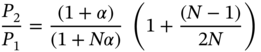
The factor α is the current ratio of fixed release overhead costs to release development costs. Fixed overhead costs include release regression testing and deployment costs, including the cost of any field testing.
Figure 8.4 shows the productivity ratio for release cycle time reduction factors of 1–12 with release overhead cost ratios of 10%, 20%, and 30% as shown in the legend.
The top line shows that productivity is lower for release reduction factors greater than 5 if the fixed overhead cost of each release is 10% of your development cost. Note how quickly the advantage of releasing more frequently is eliminated for increasing release overhead costs, stressing the importance of reducing release overhead costs to take advantage of Agile development.
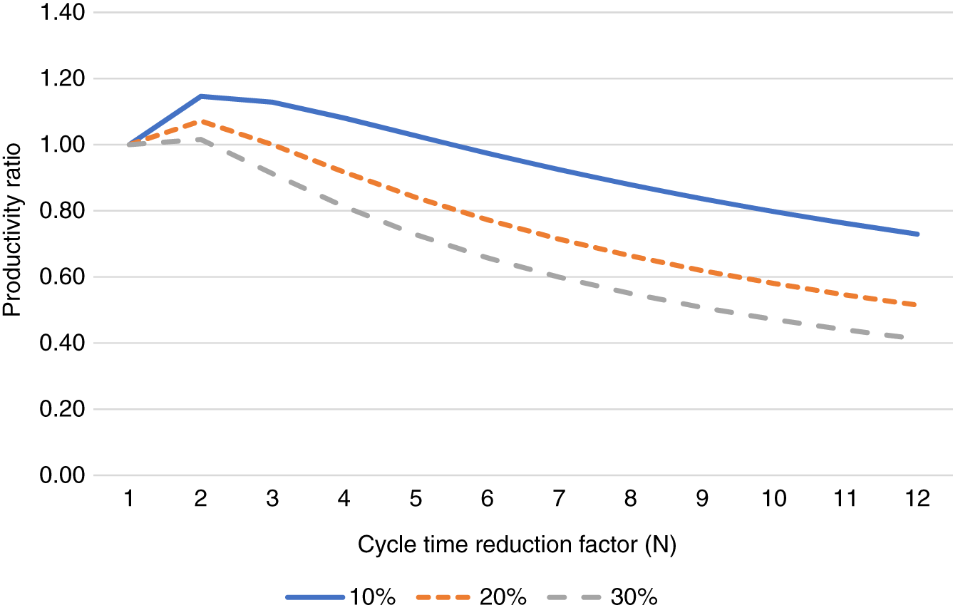
Figure 8.4 Productivity ratio as a function of release overhead cost and cycle time reduction factor.
Many companies' regression test suites have grown out of control. Functional test organizations are usually blamed for every defect that escapes. They typically respond by adding a regression test to prevent that specific defect from escaping again. Regression test libraries grow, resulting in major maintenance effort and costs to keep them current. The costs to automate these tests become overwhelming, and automation never gets done in many organizations. However, I'm not going to recommend automating regression tests as your first step.
You want to first reduce functional regression tests while maintaining or improving quality. This may appear counterintuitive, but you need to accept that maintaining large regression suites to debug software will not give you the result you expect. It turns out that only a fraction of software defects can be found at the functional testing level. This has been verified by a well‐known software engineering metrics expert named Capers Jones, and this applies to Agile development as much as it did for Waterfall.
Capers Jones defines defect removal efficiency as the percent of defects found during a specific testing phase. He reports removal efficiencies by industry for different phases of testing. He reports that even industries with the highest reliability requirements attain defect deficiency removal rates of only 30% with functional testing [1]. His conclusion is that software defect removal should be efficient at every quality verification step, including reviews, code inspections, unit and integration testing.
Functional testing also applies in Agile development. Agile development practices include creation of user story acceptance tests prior to inclusion in the sprint backlog. These are typically functional tests that can be demonstrated to a product owner. Many organizations also perform functional testing at the feature level once a set of user stories has been completed. It doesn't matter whether you embed testing within an Agile team. Functional testing is a separate activity, and as in Waterfall, people believe that all remaining defects can be detected.
There is an explanation for the limited ability to detect software defects at the functional test level. Ask any experienced developer who has delivered highly reliable software about the fraction of his or her code executed for the success path. I get responses of 20–30%. This agrees with my experience as a developer of telecommunications software with stringent reliability requirements. The bulk of the code handles cases off the “happy path,” most of which can't be simulated at the functional test level. Reasonable code coverage can be attained only with formal unit and integration testing where sets of data patterns are executed by the code. There is no shortcut.
Manual regression testing at the functional test level is expensive and time‐consuming. Defects caught at this stage are more expensive to fix and are more likely to delay releases. The subject of defect prevention and early removal is addressed in Chapter 12. It shows that you will need to increase unit and integration testing to reduce rework costs. Automate unit and integration tests first. Functional regression testing should focus on requirements verification instead of debugging. This will result in fewer functional tests to automate and execute, thus reducing release overhead costs.
After addressing release testing overhead, the next issue is the cost of deployment. This is an issue whether you or the customer hosts the application. For internal hosting, your IT department incurs costs to update and verify servers. Internal installation and testing costs are incurred for customer upgrades. Many organizations live with clunky and inefficient installation procedures. I've found that engineering, IT, and field services know what needs to be done. The problem is that their ideas never get implemented because new features are always deemed more important. Deployment improvements can now be shown to reduce quantifiable release opportunity cost as Investments.
DevOps has been a positive step toward simplifying installation, but the focus is often on increasing the efficiency of development teams. Draw the boundary of responsibility for your DevOps to address customer deployment, including the processes your customers use to support and test upgrades. The reduction in Net Cost of Delay can then be reinvested in DevOps.
And if you want to make a major dent in on‐site testing costs, improve the quality. On‐site testing is usually extended to long periods by encountering defects. As discussed above, you need to improve the quality as a precursor for cycle time reduction.
8.3 Overcoming Modular Release Challenges
Legacy software architectures make it difficult for Agile teams to develop concurrently. New functionality may impact a slice of architecture, from UI to business logic to database. The chances of overlap in common software modules are high. This needs to be addressed with architectural improvements. Modular releases also pose configuration management challenges that need to be addressed.
8.3.1 Architecture for Modular Deployment
Service‐oriented architectures (SOA) have evolved to make data from enterprise architecture more accessible. Microservice architectures have become popular in recent years. The difference is that Microservices expose application functionality and data at the Application Programming Interface (API) level. Microservices are at a lower level to provide developers with the flexibility they need to add functionality in legacy systems. Microservices can be used to implement enterprise SOA, but they are not the same. SOA are about external data access. Microservices improve development efficiency.
Most engineering departments are familiar with Microservices architectures and have long advocated them to product management. Implementation usually takes a backseat to new features. Investments in architecture to increase deployability and reduce cycle time can now be justified in terms of release opportunity cost reduction.
8.3.2 Configuration Management
Even if software functionality can be delivered in independent modules, changes to the legacy software base are often necessary. For example, new Microservices may be required to support new modules that impact the same back‐end software and data schema. We want to avoid having to support multiple versions of legacy software.
The solution is a platform approach where base software upgrades can be deployed without impact on customers. Impacts from planned Investments can be collected and implemented in a new version of base software. Periodic platform releases that don't impact functionality can be seamlessly deployed to synchronize the infrastructure software base, eliminating maintenance of earlier versions. Your platform has a release cycle separate from the delivery of functionality. Again, quality is the gating attribute.
8.4 Release Investment Prioritization
You may be wondering why we want to prioritize Investments bundled within a release when they are all released at the same time anyway. We want to be able to take advantage of the agility provided by Agile development to include new opportunities that arise during the release development cycle. Developing in WSJF order ensures that releases truncated due to schedule overrun have the highest value Investments.
T‐shirt sizing used for feature prioritization can be applied to Investment prioritization when individual Investment pricing is not possible. As with feature prioritization, T‐shirt sizes of XS, S, M, L, and XL create a linear scale with points of 1, 2, 3, 4, and 5, respectively. Relative contribution to release value is calculated in Table 8.2 using the AccuWiz examples.
As we did in the feature case, income can be apportioned based on the T‐shirt size. The same logic is used when assigning T‐shirts sizes. “To what degree does this Investment contribute to the release income?” Relative income contributions can be calculated for an example of three‐year release income estimate of $3.5M (see Table 8.3).
Table 8.4 is based on the estimated income of each Investment from Table 8.3. We assume that the Cost of Delay is proportional to the income generated by each Investment over a three‐year period and use the total three‐year income to calculate the relative WSJF. We use WSJF in the Investment case rather than ROI in the feature prioritization case because Investments are timeboxed so we know target cycle times.
Table 8.2 Relative Investment release income contribution based on T‐shirt sizes.
| Investment | T‐shirt size | Weight | Relative income contribution (%) |
|---|---|---|---|
| Quick Close | S | 2 | 20 |
| Workflow Enhancements | M | 3 | 30 |
| European Version | XL | 5 | 50 |
| Total | 10 | 100 |
Table 8.3 Release income contribution example.
| Investment | Relative contribution (%) | Release income contribution ($K) |
|---|---|---|
| Quick Close | 20 | 700 |
| Workflow Enhancements | 30 | 1050 |
| European Version | 50 | 1750 |
| Total | 3500 | |
Table 8.4 Investment WSJF priorities.
| Income contribution ($K) | Cycle time (mo) | Relative WSJF | |
|---|---|---|---|
| Quick Close | 700 | 3 | 233 |
| Workflow Enhancements | 1050 | 2 | 525 |
| European Version | 1750 | 3 | 583 |
T‐shirts sizes can be changed during release development with new information to optimize development order for Investments that are not yet completed. The relative WSJF calculation creates incentives to maximize value and minimize development effort throughout release development.
8.5 Reducing Software Inventory Costs
WIP and tie‐up of capital were discussed in Chapter 5. There is another component of WIP cost in manufacturing. Manufacturing has two categories for inventory costs. The first is the WIP inventory, which is analogous to the money invested in incomplete Investments. The second is finished goods inventory, which is analogous to the capital tied up in a completed Investment that has not yet been released. Investments waiting for release are effectively “in the warehouse awaiting shipment.” Inventory cost is the sum of manufacturing WIP and finished goods inventory. Even though finished goods inventory does not appear on financial reports as it does in manufacturing, software “finished goods inventory” should be tracked and minimized to free R&D capital.
Inventory costs for unreleased Investments should technically include costs outside of R&D, like the cost of labor and materials to create a training guide and marketing collateral. This would create unnecessary complexity in project accounting systems. For our purposes, we can use Investment software development labor costs, which is within the control of engineering. Software labor costs represent the majority of the “finished goods” cost.
Figures 8.5–8.7 show how a company might track inventory across multiple profit and loss (P&L) centers. Figure 8.5 is the total labor cost for Investments that have been completed in each week awaiting release. It's equivalent to putting “finished goods” in a warehouse.

Figure 8.5 “Finished goods” inventory costs by profit and loss (P&L) center.
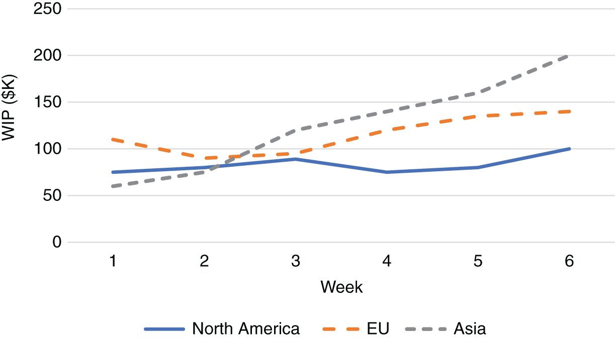
Figure 8.6 Work in progress (WIP) inventory costs by P&L center.

Figure 8.7 Total software inventory costs by P&L center.
Release inventory costs were reduced in week 4 in this example after release deployment for the North American and Asian markets. EU inventory costs continue to grow.
Investment WIP development costs can be added to the release inventory costs to show the total target for WIP reduction. Figure 8.6 shows an example of WIP development costs.
Figures 8.5 and 8.6 add to show total inventory costs (Figure 8.7).
Figure 8.8 shows total inventory costs as a percentage of annual R&D budget. It shows how effectively each P&L center is managing inventory. In this case, North America should examine why their inventory is so high relative to their annual software development budget. Is it because of inability to release more frequently, or ineffective Investment development WIP controls?

Figure 8.8 Total software inventory costs as a percent of R&D budget by P&L center.
The only action possible to reduce release inventory cost is to plan and deploy smaller releases, ideally at the Investment level. A reduction in release inventory frees R&D capital. Avoiding release bundling creates two wins: R&D capital is freed, and income is accelerated by a reduction in Net Cost of Delay.
8.6 Summary
- Bundling Investments within releases increases Net Cost of Delay because Investment income is delayed until the release date.
- Release Net Cost of Delay is the opportunity cost of not being able to deploy individual Investments.
- A general formula for productivity improvement as a function of release cycle time reduction is provided.
- Effective R&D productivity increases by 25% for each reduction in cycle time by 50%.
- There is diminishing productivity improvement for reductions in cycle time, reaching a limit of 50% for CD.
- The Investment model reveals release opportunity costs to justify development of infrastructure, tools, and processes to release individual Investments.
- Modular pricing and deployment for Investments should be adopted to leverage an installed base.
- Customers must be willing to accept more frequent releases if cycle times are reduced.
- Effective software engineering practices must be in place to achieve near defect‐free releases that customers will accept more frequently.
- A modular approach is enabled by the Investment process by limiting impacts to current customer operations and reducing customer installation impacts.
- The productivity impact of release overhead costs can be described by a formula that demonstrates the importance of reducing overhead costs to release more frequently.
- There is a point where release overhead costs for a given cycle time reduce productivity.
- The shorter the cycle time, the greater the negative impact of release overhead costs.
- Functional regression testing can only find about 30% of defects and must be complemented by defect prevention and defect detection techniques.
- Unit and integration testing should be improved and automated to reduce the number of functional regression tests before automation.
- Functional regression tests should focus on requirements verification, not debugging, to reduce the number of functional tests to automate.
- There are technical solutions to support modular Investment releases based on Microservices and platform releases.
- Release inventory costs should be tracked and minimized to free R&D capital.
Reference
- 1 Jones, C. (2008). Measuring Defect Potentials and Removal Efficiency. Software Productivity Research, LLC.