
7
Burn-In Test
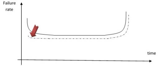
As already noted, a product that is in the manufacturing stage may typically have youth failures, notably during the first years of operation. Moreover, a product is considered mature provided that it has a constant reliability level that is higher than the specified objective. Prior to being delivered to the system manufacturer, the product should therefore be subjected to a test referred to as a burn-in test (Kececioglu and Sun 1999). The aim of this test is to eliminate as much as possible the defects generated during the manufacturing stage. It is conducted on each of the products delivered, as the manufacturing process may have certain variability and evolve (change of equipment, testing process, operator, variability in the testing means, etc.) in time throughout the period of product delivery.
In fact, for the method chosen in this book, this test is part of a more comprehensive method, namely the HALT/HASS method, which involves two distinct stages:
- – HALT testing strictly speaking involves finding the operational or environmental limits of the product in terms of thermal and vibration constraints;
- – HASS testing involves the burn-in stage.
Burn-in testing presents a challenge, however. The maximum elimination of latent youth defects at reasonable costs (notably the testing duration) requires the application of high physical contributions, significantly higher than those to which the product is subjected during its operation. While this principle may be of interest for the products with latent defects, it is not useful for healthy products (without latent defects). Therefore, it should be verified that the burn-in test does not cause serious damage to healthy products. Moreover, it should also be verified that the burn-in test has certain efficiency (capacity to reveal latent defects), otherwise it would be useless.
Therefore, prior to the actual burn-in test, two tests are conducted on a certain number of representative products of the series:
- – POS1 is used to check the minor damage of healthy products;
- – POS2 is used to verify the burn-in efficiency.
This is illustrated in Figure 7.2.
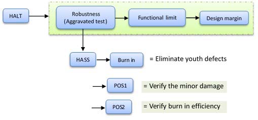
Figure 7.2. HALT/HASS testing principle
7.1. Link between HALT and HASS tests
The results of HALT tests, namely the estimation of the operational limits in temperature and vibration, can be used to give initial values for the levels of physical contributions of HASS tests. Any manufacturer willing to conduct a burn-in process must be aware of the following points referring to burn-in:
- – there is no universal burn-in;
- – burn-in is not a qualifying test. Its objective is not to validate/qualify a batch of products and therefore a technology (with an acceptance criterion such as the maximal acceptable number of defects);
- – burn-in does not aim to highlight design defects. This is instead the aim of aggravated and qualifying tests;
- – a burn-in operation must lead to breakdowns, otherwise it must be adapted. Two cases are possible:
- - if no breakdowns are detected during burn-in and operation, the manufacturing process can be considered as controlled and mature,
- - if no breakdowns are detected during burn-in, but there are youth breakdowns in the first years of operation, then the burn-in is not efficient;
- – the process should be flexible, fitted to the product.
7.2. POS1 test
POS1 can be used to verify that applying a burn-in cycle in the series stage does not damage the service life of a product by more than “X%”. Hence, one or more pieces of equipment are subjected to several cycles. The equipment undergoing this test must be very similar to those to be delivered in the final series. Under no circumstances can this equipment be delivered as operational equipment.
7.2.1. Miner’s approach
This approach is generally used in HALT/HASS tests to justify the lack of damage of the products without latent defects. The lack of damage rests on a theoretical perspective rooted in Miner’s rule (Miner 1945). According to this rule, the cumulative damage of the product is linear. Hence, if one or more products are subjected to “n” burn-in cycles without observing any failures, then the burn-in test cycle to be applied to all the products will damage the healthy products by no more than 1/n. Damage of 2% is generally admitted. In this case, the POS1 test involves the application of 50 burn-in cycles, as illustrated in Figure 7.3.
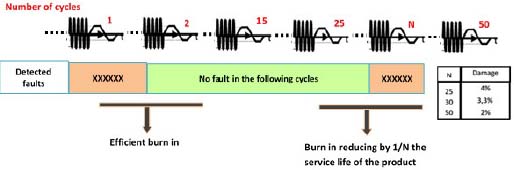
Figure 7.3. Characteristics of POS1 tests
A second hypothesis concerns the estimation of damage of products submitted to a HASS cycle. From a reliability perspective, what determines the useful service life of the product (flat sector of the bathtub curve) is the minimum of random variables representing each aging failure mechanism (that can vary depending on the life profile).
This can be schematically represented by Figure 7.4.
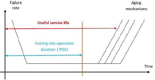
Figure 7.4. Comparison between service life and putting into service duration on the bathtub curve
If all the laws of reliability of failure mechanisms were known, it could be verified if the specified reliability objective has been met. Unfortunately, this is not the case, as the component manufacturers do not provide this information in the datasheet of the component. Though experience shows that, in general, aging failure mechanisms are not observed during product operation, the minimum of the aging mechanisms with respect to the product service life is not known. A conservative approach is therefore to take the case in which the minimum corresponds exactly to the end of the service life.
Following the failures observed during the “n” cycles, certain information can be extracted, as listed in Table 7.1.
Table 7.1. Processing of the results of POS1 tests. For a color version of this table, see www.iste.co.uk/bayle/maturity1.zip
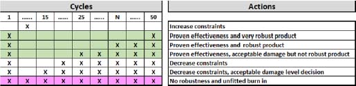
If one or several failures are observed on the first burn-in cycle, this proves a certain effectiveness of burn-in. This scenario is however unlikely given the small number of products undergoing the POS1 test. Hence, POS2 is proposed.
7.2.2. Approach according to the physical laws of failure
There is obviously no physical law of failure taking into account the simultaneous effect of the thermal cycling, vibrations and energizing. Moreover, there is no recent model taking into account the influence of the slope in the thermal cycling, this being particularly important during the precipitation phase. However, from a conservative perspective, it is possible to take into account the aging occurring during the POS1 test by considering only the effect of thermal amplitude according to the Coffin–Manson law. The focus is on the acceleration factor between the POS1 conditions and those observed during operation by the end user. This is given by:
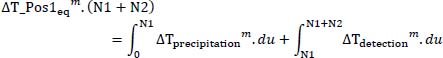
A small problem remains to be solved however, since the thermal amplitude is different between the precipitation and detection phases. However, based on the Sedyakin principle, an equivalent amplitude (Bayle 2019) can be found in terms of reliability, which is given by:
PROOF.–
According to the Sedyakin principle:
or
or
or
End
Consequently, the acceleration factor can be written as:
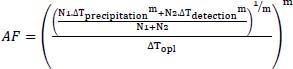
or even
Therefore, the 50 cycles of POS1 can be reflected by operational cycles in the following form:
EXAMPLE.–
Consider an operational application with the life profile given in Table 7.2.
| ΔT (°C) | Number of cumulated cycles | |
| Brazed joints | 20 | 7,300 |
| Bonding | 35 | 7,300 |
Assume the precipitation and detection phases have the following characteristics:
- – ΔTprecipitation = 150°C;
- – ΔTdetection = 110°C;
- – N1 = N2 = 2.
Let us analyze the aging generated by POS1 for the products without defects. For thermal cycling, the following failure mechanisms can be considered:
- – Breakage of brazed joints with a coefficient m = 2.
An equivalence in operational cycles is therefore obtained for POS1 for brazed joints
or
This result is below the 7,300 cycles of the life profile of the previous table. But it is important to note that the acceleration factor model that has been taken into account is very conservative. On the other hand, the focus is on the aging for one burn-in cycle. In this case, it can be seen that it represents 2,163/50 ~ 43 cycles or barely 0.6% (43/7,500).
- – Bonding removal or breakage, for active components, with a coefficient m = 4.
or
This result shows that, while being conservative, the POS1 test covers the 7,300 cycles of the life profile considered in this example. If no failures are observed, it is reasonable to believe there will be none during operation.
7.2.3. Zero-failure reliability proof approach
It is interesting to see what this means in terms of reliability for the POS1 test. Similar hypotheses to those in section 7.2.2 lead us to obtain:
- – Products without maintenance
According to equation:
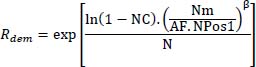
where:
NC is the level of confidence;
AF is the acceleration factor from equation [7.1];
N is the number of products undergoing POS1 test;
Npos1 is the number of thermal cycles of POS1;
Nm is the number of thermal cycles of the mission;
β is the shape parameter of Weibull law.
Resuming the data in the previous example and moreover considering that N = 4, NC = 90% and β = 5, the following results are obtained:
Brazed joints 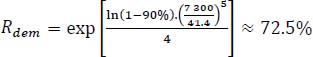
Bonding 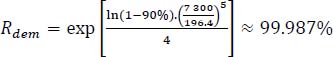
- – Products without maintenance
According to the equation:
Assuming the same hypotheses as previously leads to:
Brazed joints ![]()
Bonding ![]() 40,195 cycles
40,195 cycles
to be compared to 7,300 of life profile.
7.3. POS2 test
As already seen in the previous section, the objective of the POS2 test is to show a certain level of effectiveness of the burn-in cycle. The POS2 cycle relies on four burn-in cycles, and it theoretically damages only 8% of the healthy products according to Miner’s criterion. The four cycles are in fact a compromise between reasonable damage and a test duration that is long enough to trap as many latent failures as possible.
This test will be conducted on a series of products that could potentially be delivered to the equipment manufacturer. It is conducted in three successive stages on a certain number of products. As soon as a product is defective, the POS2 test is stopped, irrespective of the stage at which the failure occurs. Conducting the test in three stages makes it possible to limit the number of products undergoing the POS2 test if a failure is detected in stage 1 or 2.
When conducting the POS2 test, several scenarios are possible, as explained in the following table. In this table, we do not quantitatively distinguish the effect of the levels of physical contributions responsible for the occurrence of failures for each cycle. Only a qualitative analysis based on the occurrence of failures can indicate the effectiveness of burn-in testing. In the calculations that follow, the proportion of defect “p” is an unknown quantity. However, depending on the feedback for older products, a relatively accurate estimation of this parameter should be possible. The proposed process is illustrated in Figure 7.5.
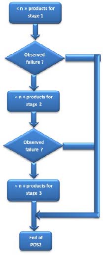
Figure 7.5. Overview diagram of the POS2 test
Table 7.3. Possible scenarios during POS2 testing. For a color version of this table, see www.iste.co.uk/bayle/maturity1.zip
All the possible scenarios are defined in Table 7.3.
POS2 testing is conducted without transfer of products from one stage to the next. Hence, it is possible to model the POS2 test by hypergeometric distribution. Hence:
- – Q is the number of products undergoing burn-in (one HASS cycle);
- – n is the number of products undergoing POS2 testing;
- – p is the proportion of products with a latent defect.
The probability of observing “k” failures is given by:
What we are interested in here is estimating the probability of having at least one failure for POS2 in order to verify the burn-in effectiveness. This probability can be written as:
or:
7.3.1. Influence of parameter Q
Let us fix p = 2% and observe the evolution of this probability as a function of Q and n. Figure 7.6 is obtained.
It can be seen that the number of products Q subjected to burn-in does not influence the probability of detecting a defect during POS2 testing. Furthermore, it is important to acknowledge that it is necessary to have a significant number of products for POS2 testing in order to achieve a reasonable probability of detecting one or more latent defects.
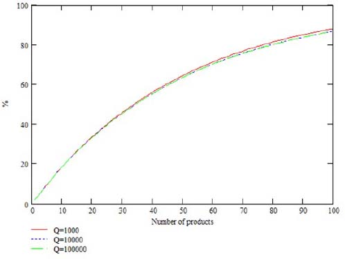
Figure 7.6. Probability to detect at least one failure influenced by Q
7.3.2. Influence of parameter p
Let us fix Q = 1,000 and observe the evolution of this probability as a function of p and n. Figure 7.7 is obtained.
It can be noted that the proportion of defects has a significant impact on the probability of detecting at least one defect during the POS2 test. Moreover, in order to have a reasonable probability of detecting a defect, the required number of products is all the larger as the defect proportion is larger, which is in fact logical.
Indeed, since generally p ≪ 1, equation [7.6] can be approximated by:
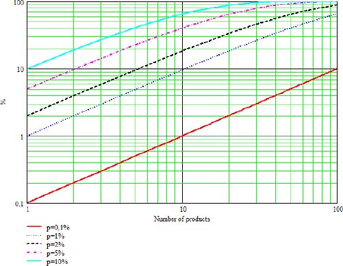
Figure 7.7. Probability to detect at least one failure influenced by p
Hence, the value of n corresponds to a given probability
Based on equation [7.8], it is possible to set a probability to filter a defect and estimate the number of products “n” that must be subjected to POS2 testing. But how can this probability be fixed knowing that it is an ascending function of n? The economic aspect can then open up a possibility. Indeed, given:
- – Ce is the cost of POS2 test;
- – Cp is the cost of a product;
- – Cr is the cost of repair due to manufacturing defect;
- – Ct is the total cost,
it can be written that:
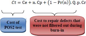
Indeed, the cost due to products having a defect depends on their number Q.p as well as on the fact that they were not filtered out by burn-in. Based on equation [7.8], it can be written that:
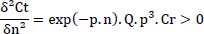
This equation is differentiated with respect to n:
This derivative is zero if:
or
or finally
Since “n” is a non-zero integer, the following inequality must be valid: ![]() .
.
NOTE.–
- – The cost of the POS2 test is not involved in the search for the optimum number of products undergoing POS2 test.
- – Due to the previous inequality, it is possible to have no optimum.
- – In case there is one, the optimum is a minimum since
- – The minimal cost obtained is given by:
EXAMPLE.–
Ce = 20,000
Cp = 200
Cr = 10,000
Q = 10,000
P = 2%
The resulting optimal number of products for POS2 test is n* = 150. The total corresponding cost is ~ 420,000.
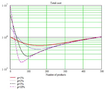
Figure 7.8. Example of cost optimization taking burn-in into account
7.3.3. Summary of the POS2 test
It should be recalled that the objective of the POS2 test is to estimate the effectiveness of burn-in. The number of products subjected to burn-in is set in advance, and therefore this parameter cannot be changed. Neither can the proportion “p” of defects; it simply remains the number of products at each POS2 stage to optimize the probability of having a failure in this test.
If no failure is observed after the third stage of POS2 testing, several hypotheses can be formulated to explain this fact:
- – The manufacturing process is excellent (p = 0.1%), and few defects are generated during this stage. The previous figure shows that with 100 products having undergone POS2 testing, there is only 10% chance of observing a failure. No conclusion can be drawn on burn-in, except that it may be useless. This situation must be confirmed by the absence of youth failures with the final user.
- – Burn-in is not at all effective and does not filter out any latent defects. Theoretically, there are 2 solutions:
- - wait for feedback information that confirms whether or not there are youth failures observed by the end user;
- - or, modify the levels of physical contributions implemented for burn-in, as they are not considered serious enough.
The general rule is to wait for the operational feedback information.
7.4. HASS cycle
Once the POS1 and POS2 tests are conducted, the HASS cycle involves two distinct stages.
7.4.1. Precipitation stage
The precipitation stage is conducted with the equipment in operation and under continuous monitoring. However, there is no need to stop the test during the precipitation stage if there are functional drifts. As a general rule, the temperature limits, HOL and LOL, during the precipitation stage are defined using the results of HALT with a 10°C reduction applied to the HOT and LOT limits:
- – high operational limit: HOL = UTOL – 10°C;
- – low operational limit: LOL = LTOL + 10°C.
A slightly different definition can sometimes be found in which the temperature limits are defined based on HALT results with a temperature reduction applied to the UTOL and LTOL limits of the HALT test defined as follows:
- – high operational limit: HOL = HOT – 10% x HOT;
- – low operational limit: LOL = LOT + 10% x LOT.
In the case of thermal cycling (type RCT), the temperature ramps are fixed at the value found during the tests for the VRT limit search; this can go up to 60°C/min in the chamber per piece of equipment (10°C/min locally on the burnt-in material). These temperature ramps are instructions of the HALT/HASS chambers (QUALMARK type). It is important to instrument any equipment confined without forced ventilation. In general, the maximum value reached is 35 to 45°C/min at the product level.
The vibration limit HV during the precipitation stage is determined from the HALT test and is decreased by 50%: HV = HVOL/2. It is important to instrument the equipment when several pieces of equipment are in the chamber in order to verify the homogeneity of vibration levels after installations.
7.4.2. Detection stage
In the detection stage, the constraints are generally applied at the specification level, making it possible to evidence obvious defects. The detection stage is conducted with the equipment under operation and under monitoring. The high and low limits of temperature during the detection stage rely on the maximal operational specification levels, and there is no notion of margin.
The temperature ramps can be weak, for example, 3°C or 10°C per minute if the equipment is to be tested during these ramps. The higher limit of vibration is reduced by 60 to 80% of the value fixed in precipitation, with the definition of a minimum level generally of 5 Grms, below which there is no descent.
The applied vibration can have a sawtooth form, ascending and descending by 5 Grms to X% of the value fixed in precipitation or in a constant manner.
At the end of each level, there is an on/off stage that may involve the rated voltages and currents as well as, in certain cases, with the minimum, maximum levels of voltage and current.
Figure 7.9 proposes an example of the HASS cycle that combines temperature levels and random vibrations.
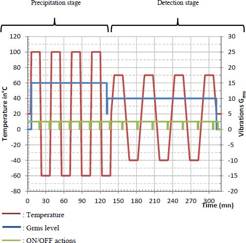
Figure 7.9. Example of burn-in cycle according to HALT/HASS method
The overall HALT/HASS method is illustrated in Figure 7.10.
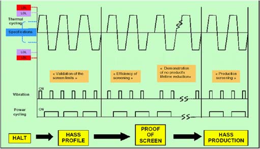
Figure 7.10. Illustration of the stages of the HALT/HASS method. For a color version of this figure, see www.iste.co.uk/bayle/maturity1.zip
7.5. Should burn-in tests be systematically conducted?
At first glance, the cost of a manufacturing process with burn-in seems higher than that of a process without burn-in. The overall cost must nevertheless integrate the costs induced by youth defects, which makes it possible to highlight the economic interest of burn-in.
We should therefore ask the question whether implementing a burn-in process is cost-efficient with respect to the objectives set. Implementing a burn-in process may be wise if the manufacturer expects to improve the following points:
- – monitoring the possible drift of manufacturing;
- – decrease of the number of refused acceptance tests;
- – reduction of the number of failures at the expense of the manufacturer;
- – reduction of the logistics due to the decrease in the number of failures;
- – preservation/improvement of the brand image.
Economic criteria are completed by certain manufacturing constraints that can guide the choice of conducting a burn-in test or not.
7.5.1. Constraints extrinsic to the equipment manufacturer
Several constraints extrinsic to the equipment manufacturer can be considered:
- – recommendation of the system;
- – operational context (life profile, production volume, etc.);
- – a diminished brand image in front of the client;
- – the seriousness of the operational life profile;
- – existence of strong competition.
7.5.2. Constraints intrinsic to the equipment manufacturer
Several constraints intrinsic to the equipment manufacturer can be considered:
- – recommendation by the company strategy;
- – cost constraints in the case of poor reliability of the product being operated by the client;
- – very demanding reliability objectives;
- – the quantity of products to be delivered.
Hence, the economic criteria and the manufacturing constraints guide the choice for or against a burn-in process.
7.5.3. Decision criteria
The overview diagram given in Figure 7.11 proposes a certain number of qualitative manufacturing criteria that may influence the decision of the equipment manufacturer to implement a burn-in process. Other criteria and constraints may be involved in the final decision (see below).
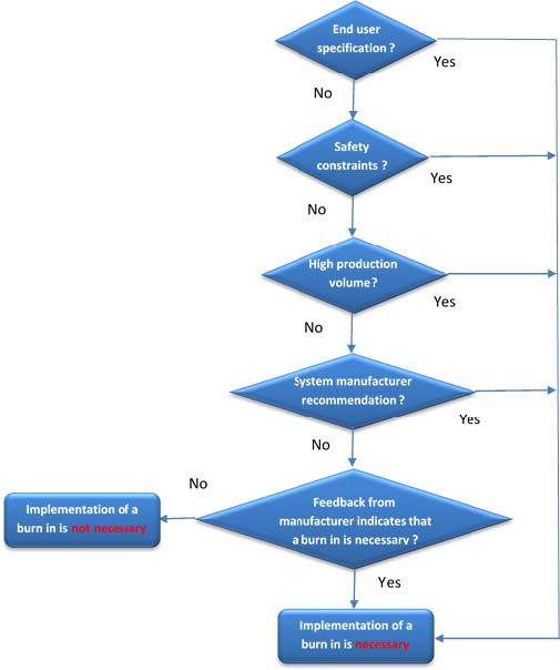
Figure 7.11. Overview diagram of decision-making
- – Final user specification:
The final user can, according to their own experience, require a burn-in test to be conducted and include it in the specifications they send to the manufacturer. In this case, it is a contractual demand that states the necessity for the manufacturer to conduct a burn-in test. This situation is typically encountered in the case of space equipment, in applying the ECSS standards required by the users. If not specified by the final user, the choice in conducting a burn-in test is made according to the other criteria given in Figure 7.11.
- – Safety constraints:
If the manufactured equipment/product is such that:
- - a high reliability level of the full product is required (typically civilian avionics);
- - if it is defective due to a youth failure, it endangers the operation of the complete product, a burn-in process should be implemented, which will eliminate a maximum number of youth defects in order to reach the required reliability level.
- – Production volume:
If the manufacturer has the elements described in section 7.5.3 available, it is possible to calculate if implementing a burn-in process is of interest, depending on the number of parts to be manufactured. Indeed, depending on the coverage rate, the effectiveness of the burn-in process and the proportion of products with latent defects, the minimal quantity to be produced before detecting a defect may be higher than the overall production. In this latter case, implementing a burn-in process presents no interest. If the manufacturer does not have sufficient elements, the choice of conducting a burn-in process is made according to the other criteria in Figure 7.2.
- – System equipment recommendation:
If the equipment/manufactured product is integrated by a system manufacturer before delivery to the final client, it can, depending on its own experience, or in response to client demand, require the implementation of a burn-in and include it in the specifications it sends to the manufacturer.
- – Feedback from the manufacturer:
In the absence of demands or external elements leading to the implementation of a burn-in process, the feedback from the manufacturer on similar products/equipment can be used to guide its choice. If for a product/equipment of similar complexity, involving identical manufacturing processes, burn-in implementation has previously revealed a level of latent defects that was unacceptable with respect to the reliability level expected for the new product, a burn-in process would logically be once again implemented.
- – Interest of burn-in implementation:
This analysis can be conducted when parameters such as coverage rate, effectiveness and proportion of products with latent defects are known or estimated.
The precondition for burn-in implementation is to have the possibility to observe products with youth defects during burn-in.
Several parameters are involved in this case:
- – the volume N (quantity) of products to be delivered. This is a purely deterministic quantity known in advance;
- – the coverage rate τc of the monitoring implemented during burn-in. This is the capacity of burn-in to be able to observe a product failure. This quantity is estimated;
- – burn-in effectiveness τeff, meaning its capacity to transform a latent failure into an obvious one;
- – the proportion p of products having a latent failure induced by the manufacturing process. This quantity is difficult to estimate precisely, as it may vary throughout the manufacturing process (variability of means, operators, components, etc.).
The number of products Q for which a manufacturing defect can be revealed can then be estimated by:
The proportion of products Pr for which a manufacturing defect is observed is then:
For the probability of observing defects revealed by burn-in to be as high as possible, it is our proposal to estimate the lower bound of this proportion Pr for a given risk level α (Gau 2010).
This is given by:
where qF is the quantile of Fisher–Snedecor distribution (Gau 2010).
The quantile of a distribution law is a reciprocal function of the corresponding distribution function. The quantity of the Fisher–Snedecor law can be easily calculated, for example, using Excel with the function “INVERSE.LOI.F”.
Hence, if N = 100, α = 10% and Q = 2, the proportion of defects amounts to 2%, but the lower bound at risk α = 10% amounts to 0.36%. The lower bound of the number of products having a youth defect revealed by the burn-in can now be estimated by burn-in from the following relation:
EXAMPLE.–
Given the following data:
- – 20 < N < 100,000
- – τc = 90%
- – τeff = 80%
- – 1% < p < 10%
The curve shown in Figure 7.12 is obtained.
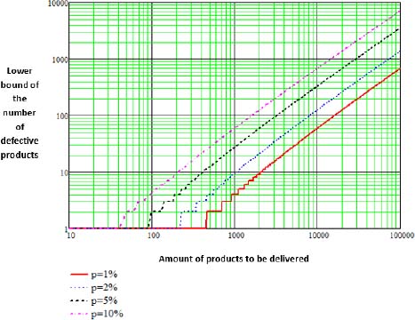
Figure 7.12. Lower bound of the number of defective products
Hence, estimating that p = 5%, a burn-in presents interest provided that the number of defective products is above 100. Moreover, for a total of 100,000 products installed, even with a defect proportion of 1%, 677 defective products could be detected over the 1,000 products generated by the manufacturing process.
Obviously, while the amount of products to be delivered is known, the proportion of defective products cannot be known in advance. However, a reasonable estimation is possible due to the experience with products from previous generations. Setting a minimum of 10 potentially defective products, the curve shows that the least number to be delivered are:
- – 200 products if the proportion of defects is 10%;
- – 500 products if the proportion of defects is 5%;
- – more than 1,000 products if the proportion of defects is 2%;
- – more than 2,000 products if the proportion of defects is 1%.
7.6. Test coverage
Throughout the manufacturing stage, a certain number of tests with various objectives are conducted. It is important to know the coverage of these tests, meaning the capacity of a test to detect manufacturing defects.
This is referred to as the test coverage rate.
Indeed, it is important to be able to precipitate the latent failures into obvious failures, but it should be possible to observe the latter, hence the importance of the test coverage.
In general, the client requirements specify a certain coverage rate of the tests, but only during the operation stage. Nothing is specified during the manufacturing stage and, strictly speaking, it is up to the equipment manufacturer to propose certain demands on this subject.
This is not always (or often) done on each of the tests implemented during the manufacturing stage, and there is no dedicated generic methodology.
According to the general definition of coverage rate of a test, the following definitions are applicable:
- – Coverage rate of the manufacturing process
Ratio between the number of defects detected by the test and the number of potential defects. Here, the term defect refers to a defect induced by the manufacturing process (improper component, missing component, improper value of the component, etc.).
- – Coverage rate of the burn-in test
Ratio between the sum of failure rates of the failure modes detected by the burn-in process and the failure rate of the product.
- – Coverage rate of the acceptance test
Ratio between the failure rate of the failure modes detected by the acceptance test and the failure rate of the product.
NOTE.– The various failure rates result from analyses of predictive reliability.
- – Industrial application
Indeed, a space application (such as Ariane rocket) does not have the same level of demand as a “consumer” application (e.g. mobile telephone).
- – Manufacturing stage
Each manufacturing stage has a specific objective, and the demand and the method for estimating the coverage rate is different.
Nowadays, the notion of coverage rate is present for the receipt test but not always for the other stages of the manufacturing process. The coverage rate results from the FMEA analysis for the qualitative part and from the predictive reliability analyses for the quantitative part.
The following definitions are proposed:
- - Potential failures: any type of failure concerning the components of the tested product.
- - Failures without effect: any type of failure that has no operational effect on the product.
- - Detected failures: any type of failure that could be detected by the implemented test.
The coverage rate of a test is generally defined by:
However, this definition does not seem to provide enough information, and it is preferable to associate it with the testability rate of the test, expressing the ability of a product to be tested. Moreover, a definition of the effectiveness rate of a test is proposed, which characterizes its capacity to detect detectable breakdowns, hence the following definition:
This definition is often used in the notion of coverage rate of a test.
7.7. Economic aspect of burn-in
A proportion “p” of products is considered to have youth defects. Consider an overall cost C(t) comprising the following:
- – fixed costs of burn-in;
- – hourly costs of burn-in;
- – cost of repair of the defective products subjected to burn-in;
- – cost of repair of defective products during operation.
The following notations are made:
- – CSP: fixed costs of burn-in;
- – CTP: hourly costs of burn-in;
- – CHP: cost of repair of the defective products subjected to burn-in;
- – CFS: cost of repair of defective products during operation;
- – Tb: burn-in duration;
- – Texp: operational duration;
- – τc: burn-in coverage rate;
- – N: number of products to be delivered;
- – fw: density of probability of a product having a youth failure, modeled by a Weibull distribution of parameters η and β;
- – Fw: probability of failure of a product having a youth failure according to the Weibull law;
- – fe: density of probability of a product that has no youth defect, modeled by an exponential distribution of parameter 1/MTBF;
- – p: proportion of products having a youth defect;
- – f˂i˃: convolution product “i times by itself” of the density of probability f;
- – N1(t): average number of breakdowns of the products with youth defects;
- – N2(t): average number of breakdowns of the product during operation.
7.7.1. No burn-in test is conducted
The overall cost induced by the products depends on:
- – the repair cost C1 during operation of products having youth defects or:

- – the repair cost C2 during operation of products having no youth defects or:
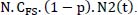
The overall cost is therefore given by:
or even:
The average number of breakdowns N2(t) during operation for the products without manufacturing defects can be calculated using the Poisson process theory. Indeed, the observed catastrophic breakdowns can be modeled by an exponential distribution of parameter λ. Considering the effect of maintenance, a homogeneous Poisson process is obtained, whose average number of breakdowns at instant “t” is given by:
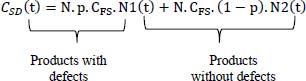
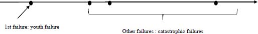
The average number of breakdowns N1(t) during operation for the products with manufacturing defects can be calculated using the renewal process theory (Bayle 2019) and is given by:
This can be illustrated with the following diagram:
7.7.2. Burn-in test is conducted
As already noted, the set of products can be divided into two categories:
- – those that have youth defects, and their number is p.N;
- – those that have no youth defects (healthy products), and their number is (1 - p).N.
Among the products having a latent youth defect, a certain number will be detected, while others will not, because the coverage rate of the tests is generally not 100%. Figure 7.13 illustrates the various possible cases for a product.
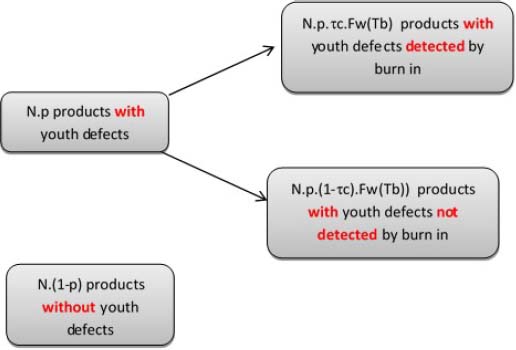
Figure 7.13. Possible scenarios for the distribution of products with or without defects
The overall cost C(t) induced by the products depends on:
- – burn-in cost given by:
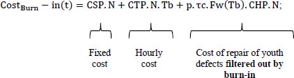
- – operation cost given by:
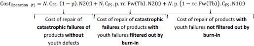
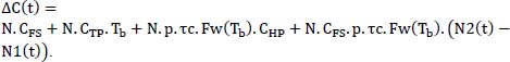
The overall cost with burn-in is: CAD (t) = Cost_Burnin(t) + Cost_Operation(t) or still:
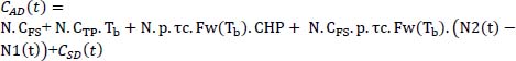
To compare these two costs, it is important to study the difference between them. Let us note this difference by ΔC(t) = CAD(t) − CSD(t) or:
The calculation of N1 is complex and requires knowledge on the parameters of the Weibull law modeling youth breakdowns. To simplify the theoretical approach, the following approximation can be made (as they are differentiated only by a youth failure):
Hence:
- – η = 1 hour;
- – β = 0.7;
- – CTP = 0.2 k€;
- – CSP = 2 k€;
- – CHP = 2 k€;
- – CFS = 10 k€;
- – τc = 90%;
- – MTBF = 1,000 hours;
- – N = 100;
- – Texp = 10,000 hours.
EXAMPLE 7.1.– Poor manufacturing process and effective burn-in:
- – p = 10%;
- – Tb = 10 hours.
The curve shown in Figure 7.14 is obtained.
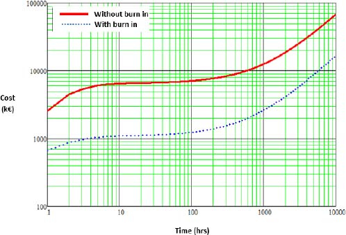
Figure 7.14. Cost of manufacturing process depending on time
The cost with burn-in is lower than that without it. This is a logical result, since there is a poor manufacturing process (p = 10%) and an effective burn-in (τc = 90% and Tb = 10 hrs). Indeed, due to the effectiveness of burn-in, most of the youth failures are filtered out and they will not occur during operation. Since the repair cost during operation is higher than that of burn-in, the overall result is positive.
EXAMPLE 7.2.– Very good manufacturing process and ineffective burn-in:
- – p = 0.1%;
- – Tb = 0.1 hrs.
The curve shown in Figure 7.15 is obtained.
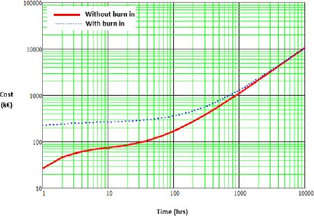
Figure 7.15. Cost of manufacturing process depending on time – example 1
The costs with burn-in are higher than that without it. Indeed, though burn-in may be effective (Tb = 0.1 hrs and τc = 90%), since the manufacturing process is very good (p = 0.1%), burn-in filters out few youth failures and is therefore more expensive.
EXAMPLE 7.3.– Very good manufacturing process and effective burn-in:
- – p = 0.1%;
- – Tb = 10 hours.
The curve shown in Figure 7.16 is obtained.
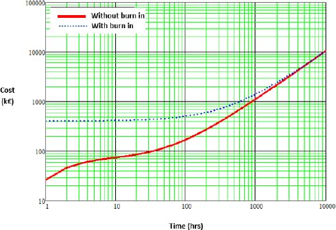
Figure 7.16. Cost of the manufacturing process depending on time – example 2
In this example, the overall cost with burn-in is higher than that without it. This is a logical result, since the manufacturing process is very good (p = 0.1%) and therefore generates only a few youth failures during operation. Hence, burn-in adds an additional cost without return on investment.
EXAMPLE 7.4.– Poor manufacturing process and ineffective burn-in:
- – p = 10%;
- – Tb = 0.1 hrs.
The curve shown in Figure 7.17 is obtained.
The costs with and without burn-in are pretty much identical. Indeed, though the manufacturing process generates a proportion of products with latent failures (p = 0.1%), burn-in being ineffective, few youth failures are filtered during burn-in.
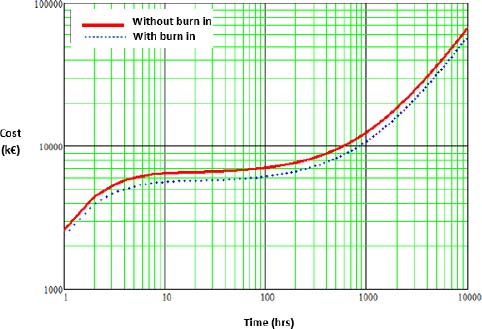
Figure 7.17. Cost of manufacturing process depending on time – example 3
- For a color version of all the figures in this chapter, see www.iste.co.uk/bayle/maturity1.zip.