Chapter 2
Digital processing
Introduction
Timecode is a digital signal. It carries information as a sequence of zeros (0s) and ones (1s), called 'digits'. These digits may represent quantities such as time or film footage, or they may carry 'command' and 'control' information. The assembly of these digits is called 'data'. Just as letters, numbers and characters have to be assembled into recognizable forms (languages) in order to be meaningful, so data must be arranged into recognizable forms in order to carry information. The arrangement of data is referred to as 'protocol'. Protocols define such matters as the number of digits used to form individual data words, the order in which data are presented within the words and the way in which the words are grouped together to carry information. There are a number of protocols used in the carrying of timecode data, depending on the application concerned. This need not be a problem because, as with languages, it is possible to translate from one protocol to another. This chapter will examine the various forms in which information may be carried within digital systems concerned with timecode, and starts by examining the nature of number systems.
The denary (decimal) system
All number systems use bases to permit a limited number of symbols to represent a large (in theory infinite) number of values. The number systems in use today use single symbols to represent quantities to a value one increment smaller than the base in use. These symbols are combined to represent higher quantities by the use of multipliers. At present most of the world communicates on a day-to-day basis using a base of 10, a number system called 'decimal' or (more accurately) 'denary'. The denary system numbers quantities from 0 to 9. So, for example, in base 10 the value 274 stands for
If a base of 5 were used 243 would stand for
(2xtwenty-fives) + (4xfives) + (3xunits) = (2x52) + (4X51) + (3x50), or 73 in base 10
Each multiplier is higher in value than the previous one by a factor determined by the base in use (ten in the case of denary). To prevent any ambiguity we should really include the base value as a suffix to the symbols used, so 274 should read 27410. As denary systems are so ubiquitous such suffixes are invariably dispensed with. When dealing with other number systems prefixes or suffixes are, however, included to make the meaning clear.
The binary system
This system uses the number 2 as its base, and so its symbols range from 0 to 1. The multiplier values are units, twos, fours, eights etc, in the everyday (denary) counting system.
So the value 11012 represents (in denary terms):
(1x8) + (1x4) + (0x2) + (1x1) = 8 + 4 + 0 + 1 = 13
Since the binary number system uses only two symbols, it lends itself readily to processing by electrical, electronic and magnetic circuitry, as the symbols 0 and 1 can be represented by such methods as the opening/ closing of a switch, the polarity of a voltage, direction of current flow or the reversal of magnetic flux. Table 2.1 illustrates some possible coding methods. As we shall see, each of the methods illustrated presents a problem that might preclude its use in timecode but, nevertheless, noughts and ones lend themselves to simple processing. As timecode uses a form of binary code, it will be as well to examine it in more detail.
With any digital system the protocol determines the number of digits required to carry the information. For example, supposing we wish to
Table 2.1 Various coding methods can be employed to store and transmit digital data.
| 0/1 indication | ||
| Coding method | Logic 0 | Logic 1 |
| Voltage level | Zero voltage | Positive voltage |
| Voltage polarity | Negative (positive) | Positive (negative) |
| Frequency shift | fl | f2 |
| Carrier phase | Advance | Retard |
| Carrier phase | Retard/ advance | Advance/ retard |
| Clocked | No clock edge | Clock edge |
| Clocked | Clock edges at bit edges | Clock edges at bit centres |
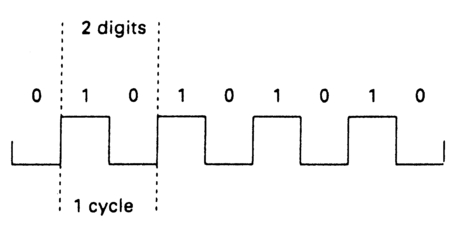
Figure 2.1 Two digits of binary information may require one complete cycle of signal.
quantify a range of weights — say a maximum of 15 g in minimum increments of 1 g — then four weighted binary digits will be required, with each digit representing a different weighted value, in this case 1 g, 2 g, 4g, 8 g. A table may then be constructed (Table 2.2) showing the arrangement of binary digits ('bits') to achieve the range of scaled weights.
Four things can be seen from Table 2.2. Firstly, each bit has a 'weighted' value which is determined by its position in the bit sequence. Secondly, the binary 'word' always contains the same number of bits, even if the leading bits are all set at zero. Thirdly, there is a maximum length to the word length, set at the design stage. Lastly, there is a minimum resolution (in this case 1 g) also set at the design stage. It is not the case, as with analogue systems, of how accurately the numbers can be read — they are present, or not present, unambiguously in the word. If higher resolution is required (or indeed if higher values than those obtainable with the set word length are required) then an extra bit will need to be added at one
Table 2.2 Digits having weighted values can signal a range of discrete values.
| Weighted binary bit values | ||||
| Denary values | 8 | 4 | 2 | 1 |
| 0 | 0 | 0 | 0 | 0 |
| 1 | 0 | 0 | 0 | 1 |
| 2 | 0 | 0 | 1 | 0 |
| 3 | 0 | 0 | 1 | 1 |
| 4 | 0 | 1 | 0 | 0 |
| 5 | 0 | 1 | 0 | 1 |
| 6 | 0 | 1 | 1 | 0 |
| 7 | 0 | 1 | 1 | 1 |
| 8 | 1 | 0 | 0 | 0 |
| 9 | 1 | 0 | 0 | 1 |
| 10 | 1 | 0 | 1 | 0 |
| 11 | 1 | 0 | 1 | 1 |
| 12 | 1 | 1 | 0 | 0 |
| 13 | 1 | 1 | 0 | 1 |
| 14 | 1 | 1 | 1 | 0 |
| 15 | 1 | 1 | 1 | 1 |
or other end of the word, which will require a complete system redesign. In a binary system, a digital word n bits long can represent values in the range 0 to 2n-1.
Commonly, microprocessors (found in edit controllers, timecode generators and timebase correctors) and digital communications systems deal in digital words eight bits long. Such groupings of eight bits are known as 'bytes'. The weighted values are as follows:
If all the bits are set to 1 the equivalent denary value is:
128+64+ 32+ 16+ 8+ 4+ 2+ 1 =255
Therefore, using a word 1 byte (8 bits) long enables all values between 0 and 255 to be identified. In this manner a range of alphanumeric and control codes can be incorporated within a single byte of digital bits.
To summarize: a word of digital bits can be used either to represent quantities (e.g. of time) by the use of weighted digits, or each combination of zeros and ones in the code can be used to represent an alphanumeric symbol or an instruction. In both cases the word length and range of values is set at the design stage.
Binary-coded decimal
Binary-coded decimal (BCD) codes are used to represent denary numbers in binary form. Table 2.2 showed that a 4-bit digital number could carry values from 0 to 15, so there is some redundancy if this were to represent a single denary number, as values 10 to 15 would not be required. A 4-bit digital word, especially one residing within an 8-bit byte, is sometimes referred to as a 'nibble'. To represent single denary numbers combining to give values from 10 to 99, two nibbles would be required: three nibbles would be required for values 100 to 999 etc. Thus the value 8710 would be represented by the bit sequence
10000111 (1000 & 0111)
Traditional (EBU/SMPTE or IEC) timecode uses a variation on BCD that accounts for the fact that not all binary words need to count to 9. The tens-of-seconds nibble needs to contain only the values 0 to 5. Where there are unused bits within each nibble, they are used to carry additional data.
Some other timecodes use longer word-lengths in order to obtain a greater range of values than permitted in ordinary BCD. For example, within the R-DAT format an 11-bit word is used to represent the number of audio samples per R-DAT frame; the EBU Radio Data System timecode uses 17 bits to represent values from 0 to 88 404 in order to store the date in Modified Julian Day form (217 = 131 072).
2's complement coding
In situations where positive and negative value binary numbers are handled (audio signal processing and EBU panscan data in timecode are but two examples) it is convenient to convert the raw binary numbers into 2's complement form. In 2's complement the MS bit signs positive or negative values, and negative value numbers are converted into a form which permits the simple addition of positive and/or negative value numbers.
Positive numbers are given a leading zero. Negative numbers are given a leading zero, '0's and '1's are inverted and '1' is added, as the following example shows:
- The value +710 converts to 01112
- The value -410 converts to 01002
- 0s and 1s are inverted to give 10112
- A 1 is then added to give 11002 (1011 + 0001)
- 710 - 410 = 3
- 01112 + 11002 = (1)00112 = 310
- The leading 1 falls out of the result.
The hexadecimal system
Reading long strings of 0s and 1s, though simple for computers, can be extremely tedious for humans. To make life simpler some digital signal processors interface with the human world by grouping digits together in blocks four bits long, and presenting the 16 possible values obtained in the form of a single symbol. This form of notation is called 'hexadecimal'. It uses the number 16 as a base, so the symbols range in value from zero to denary fifteen. Unfortunately, we do not have a purpose-built range of symbols for this system, so we use the symbols 0-9 from the denary system, and the symbols A, B, C, D, E, F to represent the denary values ten to fifteen. To reduce the possibility of confusion when dealing with hexadecimal symbols, a prefix is added to the number. This book will use the symbol '&'. The hexadecimal system of symbols with their denary equivalents is:
In the hexadecimal system each multiplier is an order of sixteen greater than the preceding one, i.e. 'units', 'sixteens', 'two-hundred-and-fifty-sixes' etc. So the value &A3F represents (in denary terms):
(10x256) + (3x16) + (15x1) = 256010 + 4810 + 1510 = 262310
In the hexadecimal system ('hex' for short) just two symbols can be used to represent any of two hundred and fifty six different values (0-255 in denary). Computers and teletex make use of this property by using these symbol pairs as codes to represent numbers from 0 to 9, upper and lower case alphabetical symbols, punctuation marks, printer instructions (carriage return, back-space etc), and a whole range of control functions depending on the protocol. These codes can be incorporated into the timecode word.
Bit rate requirements
When we come to examine the rate at which bits need to be generated/ processed for timecode, or indeed if we wish to include data other than pure time information in the code, we need to determine what information timecode requires.
Firstly, timecode requires, at the very least, the ability to carry hours, minutes, seconds and frames data — though some systems carry time data specified in increments of 1/100 frame. Secondly, we need to consider whether a complete codework will be generated for every video or film frame, or whether the time data will be distributed over a series of frames. Thirdly, we need to consider whether the data should contain timecode information alone, or whether other information, such as control signals, should be included in the codeword.
We cannot simply generate one pulse or bit per frame (as a clock may generate one tick or swing of its pendulum per second) as timecode is used to carry information other than the passing of time on a regular basis. It may be used to identify various forms of time, for example 'time from start of tape', 'cumulative recorded material time' etc. There is the matter of reading simple pulses when a machine is starting from standstill. Control track code is a simple pulse identification system. When editing using control track pulses there is frequently some slippage in the edit point as machines run up to speed from standstill. Last there is the requirement to read the code at a variety of tape speeds so that it can be read during shuttle, slow motion or 'jog' operations, or even when the tape is stationary
If a straightforward binary code were to be used to identify time, then up to 30 frames per second (fps) of information (for NTSC) would be required for every second of the day. This would require a 22-bit wordlength since there are 30 x 60 x 60 X 24 = 2 592 000 decimal number variations per day, represented by 1001111000110100000000 in binary. We could, of course, use a hexadecimal code, which would require only eight symbols (if we used one symbol for each of the elements tens-of-hours, units-of-hours, tens-of-minutes etc), but translated into a binary code at 4 bits per symbol this would require 32 bits per frame.
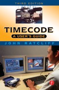
Binary coded decimal system requires 26 bits to identify each frame, as Table 2.3 shows. This is a rate of 650 bits per second (for PAL) or 780 bits per second (for NTSC). So where does this leave us regarding bandwidth requirements? If the coded bits were alternate 0s and 1s the resulting waveform might resemble a squarewave with a frequency of up to 390 Hz (Figure 2.1) as each pair of alternate 0s and 1s represents one complete cycle. Control codes are carried by the timecode word, and there may also be other factors involved that determine the data rate. The timecode may, for instance, be mixed (multiplexed) with digital stereo sound as part of a digital interface, or be multiplexed with control codes for musical instruments. (Individual forms of timecode will be examined in detail in later chapters.) No matter what information is carried, if it is to be handled by a magnetic record/replay system or transmitted at varying bit rates, we are going to have a problem with long sequences of zeros or ones as this string represents d.c. as Figure 2.2 illustrates. As we saw in Chapter 1, magnetic replay systems will not be able to replay d.c. since this involves the differentiation of the waveform. If the data rate changes because of a machine speeding up or slowing down, it will not be possible to calculate the number of continuous ones (or zeros) that have passed. The raw data will have to be modified into a suitable form before it can be processed by a magnetic system. This modification is called 'channel coding'.
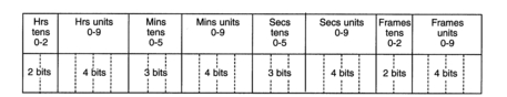
Table 2.3 Hours, minutes, seconds and frames data in BCD form can be stored in 26 bits.
Figure 2.2 A string of consecutive 1s or 0s requires the ability to handle d.c.
Simple digital codes
A number of codes are available for the processing of digital data, each with its own characteristics. It may, as we have seen, be necessary to minimize d.c. content; there may be a requirement to read the code correctly when the connector has been wrongly wired causing the data to be inverted; the code may have to be self-clocking so that it can be correctly read over a wide range of replay speeds - there will certainly be a need for all the above in codes intended for LTC. Within many digital recorders there may be a requirement for a high packing density of the digital data.
A number of digital codes are of interest where timecode is concerned, and these will now be examined.
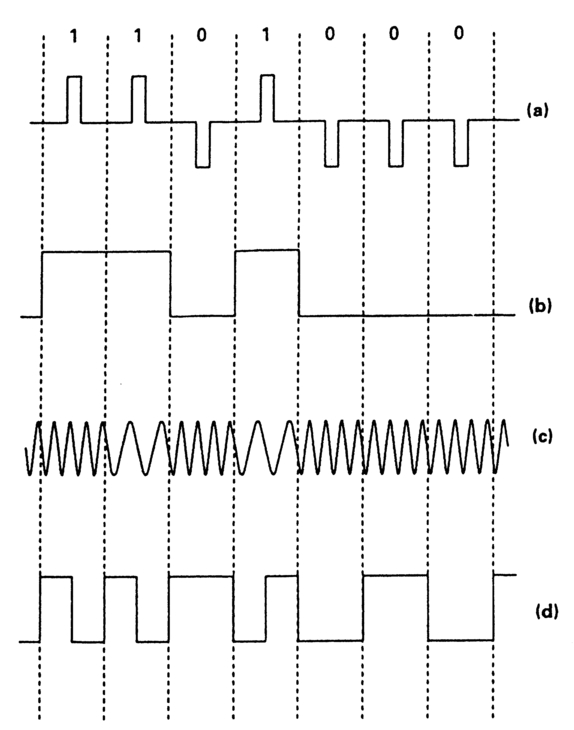
Figure 2.3 Return to zero codes (a) are self-clocking but require 3 identifiable levels. Non-return to zero codes (b) are more robust but are not self-clocking. Frequency shift keying (c) requires a wide bandwidth. It is not polarity conscious, unlike RZ and NRZ codes. Biphase mark code (d) is self-clocking and not polarity conscious.
Return to zero (RZ) code
Illustrated in Figure 2.3a, this code uses three levels or states. These can be implemented in magnetic record/replay systems by using polarity reversal of recording current to identify 0s and 1s, with zero current representing absence of data. This code will be self-clocking, but it is not immune from phase reversal resulting from connector pins being reversed, since the positive and negative data pulses will be inverted. It has found a use in the EBU / IRT timecode for 16 mm magnetic stripe film.
Non-return to zero code
This is illustrated in Figure 2.3b. This code has just two states. Polarity reversal indicates 0s or 1s. The code is not self-clocking since there is no way of distinguishing a run of 1s or 0s at other than a known speed. The code is subject to differentiation on replay. It is also polarity-conscious: if a connector is reverse-wired the ones and zeros will be inverted. These features make it unsuitable for direct recording of data on audiotape, but it is used for VITC, where the record/replay speed will be known (since the write /read speed of a helical scan video head is virtually independent of linear tape speed for a given format), where there is no possibility of polarity reversal, and where the recording system avoids signal differentiation on replay.
Frequency shift keying (FSK)
FSK code uses different frequencies to represent different logical values. For timecode with just two values (0 and 1), two frequencies will be required. Since specific frequencies represent specific logic levels, filters can be used to improve noise immunity, though this will prevent the recorded code being read at other than standard play speed. This code also has a poor packing density since several cycles will be required per logic digit for decoding. The code is illustrated in Figure 2.3c.
FM or bi-phase mark code
Originally known as Manchester-1 code, this is used for longitudinal timecode. It is, in effect, the limiting case of frequency-shift keying. It is d.c. free and self-clocking. There is always a transition on a clock edge, and an additional transition between edges to indicate logical 1. It is illustrated in Figure 2.3d. It can be read over a wide range of play speeds, hence its use for LTC, although its packing density and immunity from timing jitter are poor. The code is not polarity-conscious, as it is the presence or not of a transition that indicates 1 or 0.
Organization of digital data
One big advantage of processing information in digital form is that a series of 0s and 1s can be processed very easily, and at low cost, by electronic switches. Data can be handed on from one switch to the next very easily, and can be fed out from the system at a regular rate under the control of an electronic clock. Figure 2.4 illustrates the processes.
To facilitate the above processes it is convenient to organize the data stream into digital words or blocks, each of which has a known length and contains information identifying the start (or end) of the word. It might also be provided with some form of digital 'address' that will enable it to be placed correctly in the data stream in the event of the data words not being stored in order of time precedence. Figure 2.5 illustrates some common forms of data organization. The details of the LTC word will be covered in detail in Chapter 3.
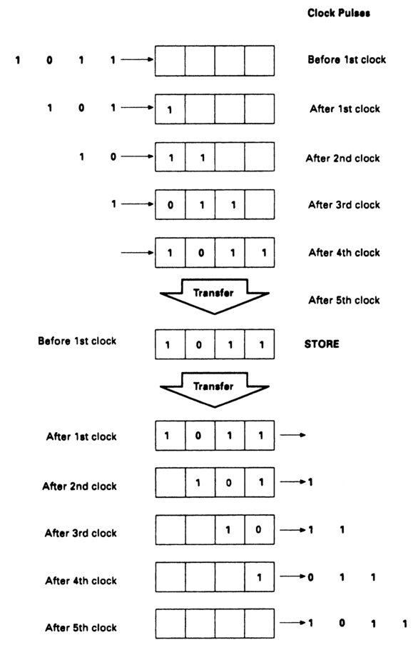
Figure 2.4 Digital data can be clocked into a shift register, then stored. They can later be clocked out. The clock rates need not be identical as long as strategies are employed to prevent the store from overflowing or emptying.
Causes of errors in digital systems
Errors can occur in digital processing systems for a variety of reasons. They result in data being misread, possibly with catastrophic results. Because of this, various techniques and working practices have been evolved to reduce the incidence and effects of errors. For example, checking bits may be added to each data word. These provide at the least a simple warning that a single bit has been misread. At a more sophisticated level, they may take the form of a complex code added to each data word that will detect and correct many errors; the data word may be repeated a number of times within a video frame to minimize the effects of drop-out on tape; the data may be reprocessed every time they are copied to avoid the cumulative effects of noise and distortion that may eventually corrupt the data.


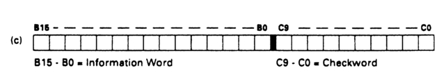
Figure 2.5 Common forms of data organization. ASCII codes carry alphanumeric and control characters in packets of 8 bits (a). Seven carry data, the eighth is parity. MIDI Header Codes comprise 1 byte divided into 2 nibbles (b). The Radio Data System packages data into blocks of 26 bits (c). 18 of these carry information, 10 perform identification and error checking.
Causes of data corruption include phase distortion, timing errors, drops in signal level, electrical noise and spurious spikes added to the data.
Phase distortion
All reactive networks, whether capacitive or inductive, introduce phase shift. At low frequency this is usually unimportant. In video circuits phase shifts are always corrected for us, as if left uncorrected they would have a profound effect on the viewed picture. The magnetic replay process also causes phase shifts because it is one of differentiation. In all cases the result is to move the timing of pulse edges.
This problem of phase shift is not pronounced for longitudinal timecode at standard replay speeds, and tape machines specifically designed to handle timecode will usually have integral re-shaping or reprocessing circuitry so that a clean rectangular waveform is present at the timecode output of the machine. However, some machines are not designed for phase-corrected replay of timecode, and an operator may well be faced with timecode on an ordinary audio track (for example, with some industrial-grade formats). In these cases the timecode should be reprocessed externally, particularly if the code is to be copied across onto another machine. Reprocessing, also known as regenerating, completely cleans up a digital signal as long as the data have not been corrupted. Pulse edges are reshaped, noise and unwanted transitions (spikes) are removed, and timing errors minimized. Reprocessing should be thought of as a preventative measure rather than a cure, though as we shall see in a later chapter, reprocessing may be used to repair corrupted data. There is the possibility that noise reduction circuitry can cause unwanted phase shifts, so noise reduction should be switched off on any track being used for timecode.
Timing errors
Plainly, if a tape is to be replayed at other than standard speed (or at least within a few per cent of standard speed) the digital data are not going to be read at the correct rate. Most timecode readers will accept data over a wide range of spooling speeds, and feed it out at the standard rate after reprocessing. They may cause timecode numbers (addresses) to be repeated if the replay speed is slow, and can result in gaps in the addresses at high spooling speeds. Where timecode data are recorded on the helical tracks of videotape or R-DAT machines, the read head may scan more than one recorded track when playing at other than standard speed. In some formats it is possible for the timecode to be distributed among the programme data in such a way that it can be re-assembled (R-DAT is such a format); in others the replay head(s) can be dynamically repositioned to follow the recorded tracks.
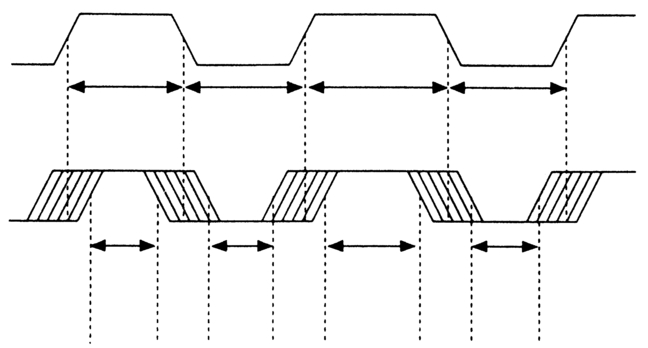
Figure 2.6 Timing jitter reduces the time window during which data may be read unambiguously.
One major cause of timing errors at standard speeds on helical scan machines is small variations in tape speed due to 'flutter'. Magnetic tape is slightly elastic; as it passes in front of tape heads and fixed guides, friction causes a stick-slip effect which superimposes small high-frequency variations on the standard speed, called 'jitter'. Figure 2.6 illustrates the effect on timecode pulse edges. The decision-making elements in a digital system have a certain latitude of replayed level beyond which the result is improbable. Timing jitter will reduce the window still further, as Figure 2.7a shows. The combination of timing jitter and partial dropout results in a trade-off between the two, known as the 'eye height' (Figure 2.7b). Any pulse transition falling outside this clear area of the 'eye' will result in possible misreading. If the misread bit was weighted to contain a significant proportion of the total value the result could be catastrophic.
All tape record/replay systems suffer from this problem, and, as we have seen in Chapter 1, video replay machines are equipped with timebase correctors to correct for this on their video output(s). Timing errors on videotape machines can be quite severe without the picture being affected because of the timebase corrector, but an audio machine slaved to unreprocessed longitudinal timecode coming directly off the video tape can hunt in speed as it attempts to follow the varying timecode rate. The solution to this problem is either to reprocess the off-VCR timecode, or to ensure that any synchronizer interface between video master and slave audio will smooth out these speed variations so that 'wow' is not noticeably present. This subject will be dealt with in detail in Chapter 9.

Figure 2.7 Timing jitter and amplitude variations combine to reduce the clear window (a), and can be traded off against each other (b) to give an 'eye height' diagram. This will specify system performance in terms of timing stability and amplitude variation.
Drop in replay level
Longitudinal timecode is often recorded at low levels of magnetic flux (compared with, say, peak level programme material) in order to minimize crosstalk. Variations in replayed level are therefore likely to cause problems. Dirty replay heads are a major cause of dropout. This is a particular problem with some video formats because of the low linear tape speeds. At the comparatively slow data rates employed by longitudinal timecode, dropout has to be quite severe before time data is lost, but if timecode is embedded either within the analogue video signal or within the bit stream of digital programme data, then even short-term dropout can cause severe loss of code. Analogue video recording systems, as we saw in Chapter 1, have their own specific ways of coping with this eventuality. Digital systems can handle loss of data in much more sophisticated ways as there is no need to handle the signal in real time. Compressors and limiters effectively reduce the dynamic range of any signal being recorded, as do automatic level controls. Because of this they should be bypassed on any track used to record longitudinal timecode.
Spikes appearing on the data
The usual cause of spikes appearing on a digital bit stream is poor installation. It may be that electrical machinery using the same mains supply is switching on and off, putting sudden spikes or noise signals onto the mains and these are finding their way onto the data-processing circuits. There is absolutely no excuse for digital systems crashing because of mains-borne interference. If the cost of a purpose-installed technical earth is prohibitive then interference suppressors should be fitted in the mains supplies. Chapter 7 deals with the matter.
Error detection
If all preventative measures fail and data become corrupted, then some form of warning (error detection) will enable strategies to be employed to prevent the errors causing problems.
The simplest form of error detection, as far as timecode is concerned, is to check the time data in the incoming word against the time data in the previous word. If the times are not contiguous then either the incoming word has been corrupted or there is a deliberate change in the time data. A corruption to the data is unlikely to last over more than a couple of frames so the incoming data can be examined for a few frames, while the regenerator generates a contiguous set of timecode words based on the last known (assumed) good word, Figure 2.8 illustrates this. Depending on the data arriving after the discontinuity, there will be a number of options open for action. These will be examined in Chapter 7.
It is possible to include a single bit of data within a digital word, usually (but not necessarily) at the end, whose value is chosen so that there is an even (or odd) number of 1s within the word, depending on the protocol. This additional bit is called a 'parity bit'. When the codeword arrives, the number of 1s can be checked to see whether there is an even (or odd) count. This process is known as 'parity checking'. A protocol requiring an even (odd) total of 1s in the word is called 'even (odd) parity'. Figure 2.9 illustrates the principle. A single parity check cannot guarantee to detect more than one single error per word, nor can it indicate which bit is in error. The longitudinal timecode word contains such a bit. It was not intended as a parity bit, it was intended to make the join between successive codewords smoother (see Chapter 3), but it is in effect a parity bit, and as such can be used for checking the validity of the word - though whether a single parity bit is of much use to an eighty-bit word is open to debate.
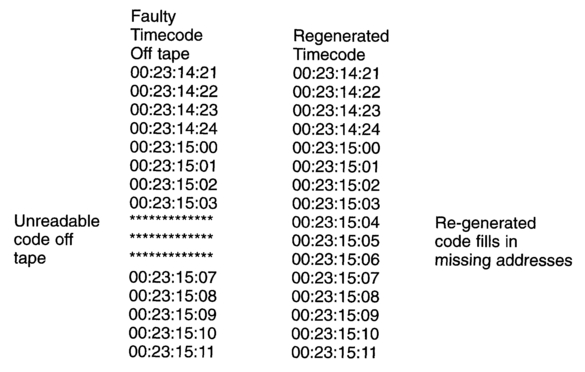
Figure 2.8 A regenerator can continue generating a contiguous series of time addresses in the event of short-term loss of code. Long-term loss can be regenerated if all devices are connected to a common set of sync pulses.
More sophisticated forms of error detection are the Cyclic Redundancy Check Code (CRC or CRCC) and the Checksum, both of which are used with various forms of timecode. Both forms of error detection involve placing a codeword on the end of the data word before transmission or recording, and using it after reception or replay to check whether the time data have been corrupted. The value of the codeword is determined by the weighted values of the digits making up the time data. CRCs and checksums are extremely powerful tools for detecting errors. They both require additional bits to carry the checking data, which has implications for the data rate. The CRCC used in Vertical Interval Timecode can detect burst (i.e. consecutive bit) errors with a certainty of better than 99.5% (misdetection is less than 1/256 for a burst error of 10 consecutive bits or more).
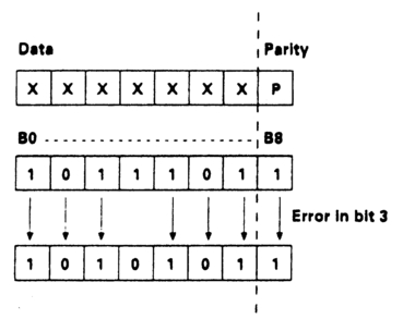
Figure 2.9 Even parity. If a single bit fails, an odd number of 1s results. This can be detected, but there is no indication of which bit has failed, nor will errors in an even number of bits be detected.