4.3

TOLLING AGREEMENTS

With deregulation, sweeping changes were made to the ownership of power plants. Power plant operators became responsible for selling power in an open market in addition to maintaining their power plants. The safe business of operating a power plant—once thought of as an ultra-secure investment—was now a very risky business. To address this new reality, power plant operators began to specialize. Some focused on maintaining the physical hardware of power plants, and others focused on marketing the power.

The general mechanism for outsourcing trading responsibility is to rent the power plant to a power marketer, a company specializing in power trading, through a tolling agreement. These agreements can run for any length of time (often 20 or 30 years) and divide the job of running a power plant between the two parties. The owner gets paid a fee to maintain the power plant while the power marketer makes all of the economic decisions. The power marketer is responsible for supplying fuel to the plant and selling the resulting electricity into a competitive market. The power marketer takes on all of the economic risks and earns all the profits above the fixed maintenance fee.

Renting a power plant gives the power marketer the ability to convert fuel into electricity. In a financial sense, this is alchemy—a power plant provides the ability to turn a low-cost commodity into a more valuable commodity. Best of all, the conversion doesn’t have to be made if it is not profitable. For example, if the spread between electricity prices and fuel prices is unprofitable, the power marketer can turn off the power plant.

This ability to not operate is very similar to the behavior of financial options. The owner of a financial option has a choice of taking an action or doing nothing. As a result, tolling agreements are commonly modeled as a series of financial options. Based on this concept, one way to value a tolling agreement is equal to the cost of replicating a power plant’s physical capabilities with financial option contracts. Approximating real behavior with a financial option model for the purposes of valuation is called a real options approach to modeling.

Converting Fuel to Electricity

Physically, power plants operate by burning fuel to produce electricity. Some power plants are more efficient at producing electricity than others—they burn less fuel to produce the same amount of electricity. The conversion efficiency of this process is called the plant’s heat rate. The higher a plant’s heat rate, the more electricity it produces for the same amount of fuel (Figure 4.3.1).

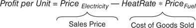
Figure 4.3.1 Profit per unit

Calculating the profit from this conversion is a standard net profit calculation—a power plant’s profit is the sale price of its product minus its cost of materials and operating costs. In most cases, since fuel costs are much larger than other operating costs, the operating costs are ignored and the net profit of a power plant is approximated only by the conversion efficiency of the power plant. For a single unit of output, this estimate of net profit is called a spark spread.

The net-profit formula for using a spark spread approximation is shown in Figure 4.3.2. This is a fairly standard net-profit formula—the number of units can be multiplied by the per-unit profit to calculate the total profit. The terminology in this formula will be used throughout the remainder of this discussion.

Figure 4.3.2 Spark spread

Since spark spreads can be negative, the ability of the power plant to turn off means that its profit needs to be approximated by a spark spread option rather than a spark spread. A spark spread option is a spark spread whose owner has the option of taking a zero profit. Taking zero profit is similar to a power plant shutting down. When spark spreads are positive, the power plant’s total profit is its per-unit profit (the spark spread) multiplied by the total units of electricity that the power plant can produce. When the spark spread is negative, the power plant has zero profit.

As a general rule, any time spark spreads are positive, the owner will take the profit. Any time spark spreads are unprofitable, the owner will try to opt for zero payment by shutting down the power plant. Occasionally real life will interfere. For example, the owner might not be able to shut off the power plant for regulatory reasons. Alternately, the power plant operator might not want to let the power plant cool down too much and would consider it worthwhile to operate at a loss for a couple of hours to avoid the costs associated with restarting a couple of hours later.

Breaking Up the Model

Because the power marketer isn’t going to make just one decision on the power plant, a large number of options are required to approximate the physical behavior of a power plant. Most commonly, a power plant will make operating decisions on an hourly, daily, or monthly basis. Typically a model of a tolling agreement will create an option for each operating decision. Each leg of the trade represents a set of decisions occurring around the same point in time. For example, a tolling agreement might be broken up into monthly pieces where a single on/off decision will be made for the month (Figure 4.3.3).

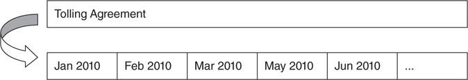
Figure 4.3.3 Breaking a tolling agreement into monthly options

Even though a model of a power plant should be based on how the power plant actually operates, there are differences between estimating future decisions and making decisions for the current day. Detailed information, like hourly prices, is not available for future periods. As a result, there is little advantage to using very small time frames if the prices have to be estimated from longer time periods. Choosing longer periods for estimating decisions can simplify a model. Most models have an optimal point of complexity. At that point, being more complex doesn’t make the model more accurate, it only makes it slower to calculate and harder to test.

The primary factor in choosing an appropriate number of legs is the availability of market data and the physical capabilities of the power plant. If the only available prices come from the forward market, which trades monthly contracts, there isn’t much benefit in choosing a daily model or hourly model. However, if some type of daily price is available from a simulation, a daily model might be better.

The physical capabilities of the power plant being modeled also have an effect. For example, a gas turbine might benefit from a high-frequency model since it can start and stop quickly. However, a steam turbine, which takes a while to get operating at top efficiency, will want to operate for an extended period. In that case, a modeler might use a longer time frame to model a steam turbine.

Underlying Instruments

The description of a spark spread model might make it seem like there are only two underlying products—power and fuel. However, this is misleading. Each leg of a tolling agreement requires electricity and fuel prices at the right time and location. Unless storage is easy, energy products are not the same commodity at different points in the year. For example, August electricity is a fundamentally different product than May electricity. It is impossible to buy some electricity in May and hold it until August.

This has a big effect on risk management—any measure that tries to aggregate risk between multiple legs has to account for fundamentally different underlying exposures. Given the extended length of many tolling agreements, there can be several hundred separate commodities being traded over the lifetime of the contract.

Even within a single leg, there is often a need for separate underlying instruments. For example, if a tolling agreement is broken in monthly legs that correspond to the forward markets, it has to be based upon the products traded in that local forward market. Commonly traded contracts in the forward market are for peak power (5×16 power), off-peak power (7×8 power), or weekend power (2×16 power). As a result, it is common for each leg of a tolling agreement to depend on a variety of different instruments (Figure 4.3.4). Combined with the time of year effect, the different daily products can rapidly add up to huge numbers of uncorrelated exposures.

Figure 4.3.4 Multiple exposures per tolling agreement

The impact of this on risk management is substantial. Because legs don’t share underlying instruments, it is impossible to simply add up the exposures to get a meaningful number. For example, it is wrong to ask: “What’s the exposure of this power plant to the price of electricity?” because there is no single price of electricity. It is dangerous to assume that all electricity prices will move together when prices have historically been uncorrelated.

Physical Model of a Power Plant

A physical description of the power plant is also required to build a tolling model. For example, a physical description might be: a natural gas combined cycle power plant with four turbines: two combined cycle steam turbines, and two gas turbines.

In this power plant, the steam turbines are large and efficient. However, they are expensive to maintain and can’t respond quickly to changing power requirements. The power plant also has two peaking generators (the gas turbines). These two gas turbines are much smaller and less efficient than the combined cycle turbines. They are used to provide heat for starting up the combined cycle steam turbines, but otherwise operate as separate units. When operating separately, since they are fairly inefficient, the gas turbines are mostly utilized during periods of peak demand.

As an approximation, the combined cycle turbines have two operating modes—normal dispatch or maximum dispatch. Maximum dispatch mode is less efficient at converting fuel into electricity, but produces more power. The operational parameters of this power plant are summarized in the chart in Figure 4.3.5. This chart shows the capabilities of each turbine installed in the power plant. Lower heat rates are more efficient and shown in units of MMBtu per MWh.

Figure 4.3.5 Operating capabilities

Both the efficiency of the plant and its total output determine its profitability. The total profitability of a power plant depends on its per-unit profit (the spark spread) and the quantity of electricity that it can produce (the dispatch rate). These two factors need to be balanced against one another. Higher levels of production are less efficient—they require more fuel per megawatt of power. As a result, the per-unit profit decreases as more power is produced.

Optimal Operating Mode

Running a power plant economically requires an optimization. Sometimes it is more profitable to produce a greater amount of electricity. This happens when the decreased profit per megawatt is overcome by the additional sales. At other times, it is more important to be extremely fuel efficient. Lower heat rates indicate a better utilization of fuel per amount of energy produced.

Most power plants are not simply on/off switches. Their value depends upon them being able to operate in the most profitable manner. Power plants typically have a variety of modes in which they can operate. Valuing a tolling agreement requires figuring out the best operating mode for each leg.

To simplify the process of determining the best way to operate the power plant, it is common to combine operating decisions for several turbines into an operating scenario. For example, it is possible that all of the units will be off, that only the most efficient units are operating, or that all of the units will be operating (Figure 4.3.6). The assumption behind these scenarios is that the less efficient turbines will never be activated before the efficient ones. The following scenarios were calculated by summing up the capabilities of generators described in the previous chart.

Figure 4.3.6 Operating scenarios

Operating Scenarios and Day/Night Power

Coming back to a point made earlier, there is often not a single price for power. There are usually several types of power prices that need to be analyzed in conjunction—for example, daytime and nighttime power. These periods will alternate, and it may not be possible to cycle the generator between periods. The value for each operating scenario will need to account for the profits in both periods.

Sometimes, turbines will need to operate at night if they are going to be active during the day. For example, steam turbines might find it impossible to completely turn off and then restart a short time later. Because of the cost associated with a restart, steam turbines might need to continue operating in a reduced capacity at night.

This creates a problem since prices on nights and weekends are generally much lower than during the day. A power plant might need to take a loss during nighttime hours to be profitable during the day. The value of each scenario needs to group profit and losses together when a single decision determines both values.

The operating scenario chart is expanded in Figure 4.3.7 to account for nighttime hours. It shows the required linkage between the day and night scenarios. For example, in the CC Max scenario, the combined cycle generators operate at maximum capacity during the day, but go to their most efficient operating mode at night to minimize the operating losses. In addition, a new scenario was added, Peaking Only. This new scenario addresses the possibility that especially low nighttime prices make the steam turbines unprofitable to operate at all during the day.

Figure 4.3.7 Additional operating scenarios

Correlation Between Electricity and Fuel Prices

A second set of problems comes from option pricing considerations. Regardless of which operating scenario is chosen, the value of the power plant will depend on assumptions about the future relationship between electricity and fuel prices. Fuel is being combusted to convert it into electricity. Wide spreads are good—cheaper fuel and more expensive electricity means higher profits. However, the future of this relationship isn’t known at the time of valuation and requires a number of assumptions to be made. For example, because no one is very good at predicting future prices, most models are going to assume each asset follows a random walk. However, because power prices are affected by fuel prices, this means that the spark spread is going to depend on the combined behavior of two random (but correlated) walks.

Since the power plant can be turned off to limit exposure, extreme moves in the spread are a good thing. Either the power plant makes a windfall profit or it gets turned off. From a profit perspective, high volatility in the electricity/fuel relationship is good. To a large extent, the value of a tolling agreement depends on the expected correlation between power and fuel prices. Highly correlated power and fuel prices mean less volatility and lower profits. Small changes to the correlation between these prices can have a major impact on the value of a tolling agreement.

Valuation and Volatility

Some of the value of a tolling agreement is known immediately. At a minimum, it is worth its intrinsic value—its value if all of the operating decisions were made immediately. This can be done by arranging firm agreements to buy fuel and sell electricity through the forward market. However, there is a second component to an option’s value. Uncertainty benefits the owner of an option. The downside risk of owning an option is capped. In the case of a power plant, the power plant can be turned off. A 50/50 chance of making extra money is a great investment when losing doesn’t involve spending more money.

The valuation date of an option is the day that its value is calculated. The expiration date of the option is the day that the power plant actually converts fuel into electricity. Up until the expiration date, it is possible to change the operating decisions for the power plant. After that date, it is no longer possible to change the decision. Exercising the option means making a permanent decision on how to operate the power plant. Usually, it is preferable to delay making a final decision on how to operate the power plant for as long as possible.

The payoff of a spark spread option is based on the spread between power and gas prices. Today’s prediction of those prices is the forward spread. The spread at the time of expiration probably won’t be identical to the spread that is being predicted today. However, it is likely to be distributed around the forward spread (Figure 4.3.8). Mathematically, the likely range of spreads is described by a statistical distribution centered on the forward spread.

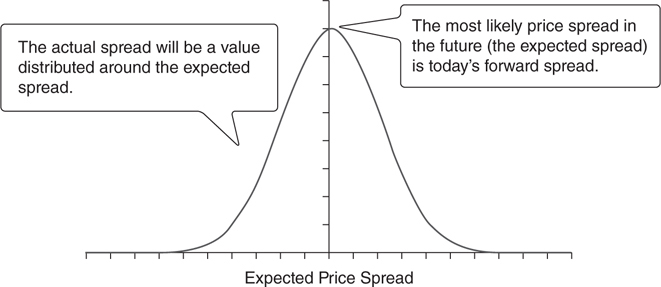
Figure 4.3.8 Expected price spread

Some of the possible spreads will be at points where it is profitable to produce electricity. Other spreads will be at points where it is unprofitable to operate the power plant. The efficiency of the power plant (its heat rate) determines which spreads are profitable and which spreads are unprofitable (Figure 4.3.9).

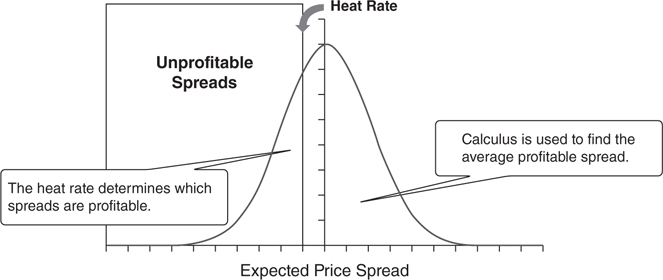
Figure 4.3.9 Heat rate spreads

At expiration, the profit per megawatt is calculated by taking the average price of the profitable future spreads. Multiplying the number of megawatts (the dispatch rate) by the average profitable price calculates the expected profit from that scenario.

The width of the distribution is a key factor in determining the profit per megawatt. A spread option is more valuable when the range of possible spreads at expiration is high. The chance for an extremely positive payoff outweighs an increased chance of losing money. This is due to the asymmetric nature of the payoffs—any loss is worth no worse than zero, but beneficial results are uncapped.

The width of the distribution depends on the time between valuation and expiration and the correlation between power and gas prices (Figure 4.3.10). If the prices of power and natural gas are highly correlated, the spread at expiration will be very close to the center of the bell curve. For example, if the prices are perfectly correlated, there won’t be a bell curve at all because the relationship between prices will never change. Less correlated assets will have a wider distribution of possible spreads.

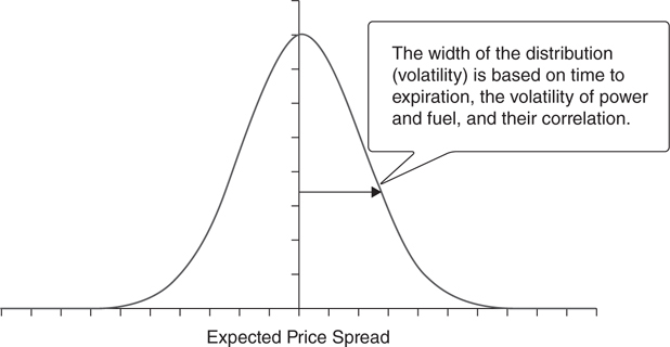
Figure 4.3.10 Volatility and correlation affect width of spread

All options are highly affected by changes in volatility. In the case of spread options, the volatility of the spread depends on the correlation between power and gas prices. As a result, the value of a tolling agreement is incredibly sensitive to the predicted correlation between fuel and power prices. Even very small changes in this correlation can have a huge impact on the value of the power plant.

Dangers to Using Options

There are dangers to using options to approximate physical behavior—a spread option model can ignore important physical aspects of generation like the time it takes to turn on (ramp up or cycle) and variable operating costs. For example, a generator might take longer and use more fuel to start operating in the winter than during the summer. Options also assume power plant decisions can be made instantaneously. No matter how quickly a power plant can be cycled, it is going to be slower than instantaneous decisions implied by a spark spread model. Other real-life issues—like the effect of local laws regarding grid reliability—can also be difficult to quantify.

Because spark spread option models are less constrained than actual generators, they run the risk of overestimating profitability. This overestimation can be as high as 20 to 30 percent if overoptimistic assumptions aren’t caught. These errors can also trickle into other systems, like value-at-risk calculations, and may not be recognized for years.

Another criticism of spark spread option models is that they are “reactive.” They assume that a generator simply turns on or off in response to the current price. In reality, the optimal schedule for a generator must anticipate price changes, perhaps incurring a loss in some periods in order to position the generator to capture higher expected profits later on. Again, there is no one single rule for handling this issue. The relative importance of this problem is different for each generator and how the operating scenarios are selected.