As with so much else, it’s useful to start off knowing what it is you are trying to accomplish. That means gathering requirements. There is some skill, perhaps, associated with gathering requirements. If you aren’t looking for actual requirements, you are going to end up with a solution in search of a problem, which isn’t very useful. Once you have the requirements and understand what you are building your lab network for, you can start thinking about how to design it. In the simplest of cases, you will find that you can stick all of your systems on a single subnet. That’s not always going to be the case, however. You may want to have a little depth to your network, which may mean multiple subnets as well as the ability to pass between them.

When you have multiple subnets, you may want to have some security controls, such as firewalls, between them. These controls will add a lot of realism to your network. This is especially true if you want to practice your penetration testing. After all, in the real world, you are going to come up against firewalls and intrusion detection systems. You will need to practice how to evade those controls. This means you will want to have installed some firewalls and maybe some intrusion detection system—perhaps even intrusion prevention systems.

Before we get around to turning on all sorts of devices, though, we need to cover some foundations about networking. No matter what platform you end up building your lab in, whether it’s physical systems or virtual systems or even cloud systems, you need a handle on how those systems communicate with one another. Since there are large numbers of books that do a great job of going deep into networking, we aren’t going to do that here. It is worth making sure we are all on the same page and doing a quick recap to make sure you remember some subject matter you may have shifted out of your near-term memory.

Networking Basics

As this is a book about setting up a lab environment and not one about networking, we’re not going to spend a lot of time on this but there are some fundamentals that will be needed here so we’ll go through them. If you are well-versed in networking, you can feel free to skip ahead to the section “Network Topologies” later, since there won’t be anything new here. For all those still here, let’s start by talking about Transmission Control Protocol/Internet Protocol (TCP/IP). TCP/IP is a suite of protocols that were developed for use on what was then the Advanced Research Projects Agency Network (ARPANET). While discussions about networking usually start with models, we’re not going to do that. We’re going to focus on TCP/IP exclusively and talk about the elements that are important for our purposes.

Network Access Layer

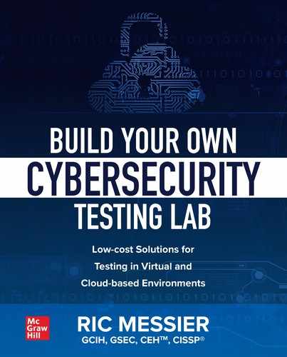
The network access layer covers two pieces of business. The first, which we aren’t going to worry about, is the act of physically connecting a device to the network. This is the cables, jacks, and other assorted materials we use to just get to the network (including the actual air, by the way, since lots of people use Wi-Fi). Instead, we should talk about the data access layer. This is where we move from electrical signals to bits. Once we move to talking about data rather than talking about electrical signal, we need to know how to get that data from the sender to the recipient. At the network access layer, this is done through the use of a media access control (MAC) address. This address is stored in the network interface card (NIC) and, as a result, is sometimes called the hardware or physical address. You can see an example of an interface configuration below, including the MAC address on the line that starts ether, which is short for Ethernet.

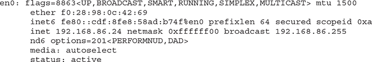
The MAC address is 6 bytes (also called octets) in length, comprising two sections. The first half, known as the organizationally unique identifier (OUI), identifies the manufacturer of the network interface card. This information is well-known and as a result is available to products like Wireshark to provide a reverse lookup on the OUI. You can see an example of this in Figure 2-1. Wireshark shows the name of the vendor for the NIC in the source address. You’ll see there is both a source and destination MAC address. Ultimately, all communication is local. No matter where the ultimate destination is, messages have to be sent to systems on the local network. You won’t know the MAC address of your final destination if the message is not local, because MAC addresses never go beyond any gateway device to another network. The destination MAC address for anything to be sent to a foreign network is the MAC address of your gateway.

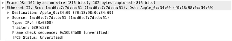
Figure 2-1   MAC addresses in Wireshark

The network space where the MAC address is relevant is called the broadcast domain. The reason it’s called the broadcast domain is because it’s a subset of devices on a network that can reach each other by sending messages to the broadcast MAC address. The broadcast MAC address is ff:ff:ff:ff:ff:ff. If I can get a message to you by sending to that address at the data link layer, you and I are in the same broadcast domain.

Devices in the same broadcast domain communicate at the data link layer using the MAC address. While the address is bound to the network interface, the address can be changed, even if it’s coded into the NIC. One way or the other, you need to know what the MAC address of a system is. We’ll get to Internet Protocol (IP) addresses shortly but for now, remember that messages going out on the network are built top down. This means the IP address is added on before the message hits the wire and since we always have to have a MAC address on the message, we have to have a way to map the IP address to the MAC address. This is handled with the Address Resolution Protocol (ARP).

ARP is a two-stage protocol. A device has an IP address and needs to know the MAC address to put the message on the wire. The system sends out an ARP request. You can see a frame, which is the protocol data unit (PDU) at this layer, with an ARP request in Figure 2-2. The ARP request has the target IP address set with no MAC address set. You can see this in the ARP portion of Figure 2-2. You can also see that the source MAC address is set, as is the source IP address. When you look higher in the message, though, you see that there is a source MAC address in the Ethernet header. We have to have a destination and the best way to get the information we need is to ask the entire network, so we set the destination MAC to be the broadcast address. The broadcast address has all the bits set, giving us ff:ff:ff:ff:ff:ff as the broadcast address. The point of sending this out is that the host that owns the IP address we want to communicate with will respond to this request and we’ll get the MAC address we need.

Figure 2-2   ARP request

You can see the response in Figure 2-3. The ARP response has reversed the sender and the target addresses. You can now see not only the IP address but the MAC address in the sender field. What you don’t see, because it’s shown in the Info column above, is that ARP requests are usually short-handed to “Who has” and ARP responses are commonly short-handed to “is at” so you don’t have to say ARP request and ARP response. The thing about ARP is that there is nothing built into it to do any sort of authentication. We assume that systems are going to behave and only tell the other systems on the network that they have the IP address they actually have. Should someone want to pretend to be the owner of an IP address, they can send out an ARP response to a request. Or, better yet, just send out a response to a nonexistent request. This is called a gratuitous ARP.

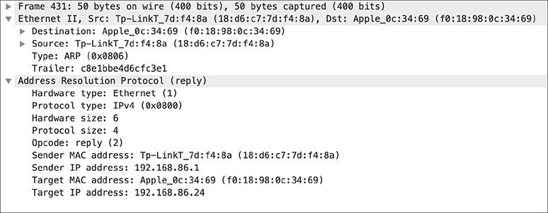
Figure 2-3   ARP response

When any ARP response passes by a system, it will be noted. This saves any system looking for that IP address later from an ARP request since it will have stored the MAC-IP mapping in an ARP table. Even gratuitous ARP responses, those that have not been asked for, will get noted. We now have a way to make the connection down the stack from an IP address to a MAC address and we know what a MAC address looks like and how it interacts with the network.

Switching

One advantage we get from the fact that we have a MAC address is that messages can be filtered using that address. While you can implement security mechanisms that make use of the MAC address, a very fundamental use of this address is through switching. Switching is the use of a physical address to redirect frames to a correct destination. There are a number of protocols that make use of this form of traffic management, including Ethernet, Frame Relay, and many others. When it comes to Ethernet, which is what you will likely be using in your lab, we can make sure only the destination host gets messages that are being sent to them. This increases performance because each network link only has messages that should be on that link, freeing up space on the link for more traffic for that particular host. Figure 2-4 shows a representation of switch and the systems that are attached to it, as well as the MAC addresses associated with systems that are running.

Figure 2-4   Switch representation

A switch is a device that makes those decisions. Today, you are likely used to seeing nothing but a switch in whatever network you are using. Before we had switches in networks, we used hubs. A hub is a dumb electrical repeater that just takes a signal coming in and repeats it out to all ports on the device, aside from the port the signal originated on. A switch uses something called content addressable memory (CAM), which is just a hash or dictionary that is implemented in hardware. With a dictionary, to get one value, you look it up through the use of another value. You have a word you want to know the definition of. So, you look up the word in the dictionary and get the definition. Typically, it’s faster for a computer to use a numbered array of values. Getting to value 15 of the array is fast because the computer knows the starting memory address and it adds on 15 times the size of the array value. You can see a representation of an array in Figure 2-5.

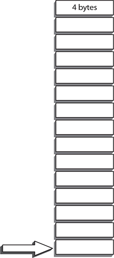
Figure 2-5   Array representation

In our case, each stored value is 4 bytes, so we multiply 15 by 4 and find that the location of the 15th position in the array is the starting address plus 60 bytes. This is a quick and easy calculation. A CAM table, though, is something else altogether. If we wanted to find the port number associated with a MAC address, we would need to look up that port by the MAC address. This is not a calculation. This is just indexing the values by the information we need to look something up by. So, if we had a MAC address of af:d3:b1:23:42:a1, we would look at the memory space referred to by that address and get, say port 5. In a programming context, it would look something like this—array[af:d3:b1:23:42:a1]. The MAC address is the index to the array, rather than a straight numeric value.

Switching allows for more efficient network communication because once the destination MAC address is on the frame, the network knows how to get that frame from one point on the network to another. This does mean, though, that the network needs to know where MAC addresses across the network are located since larger networks aren’t going to have every device on a single switch. A connection from switch to switch would carry multiple MAC addresses if frames were going from systems on one switch to systems on another switch. This gets even worse in cases where you have a large number of switches in a network and they are connected either like a star or even as a ring.

In other words, if any frame has multiple paths to get from one system to another system by way of different switches, you now need to make sure that you know the best way to get from one system to another and, more importantly, that you aren’t introducing any switching loops where a frame is sent from switch A to switch B and both of them think they have a pathway to a particular MAC address, except that it’s through each other so they keep passing it back and forth. One way to keep this from happening is the spanning tree protocol (STP). This is a protocol that will ideally keep loops from happening.

The switch is only one device that can be used to move messages around the network. You will also run across bridges, which pass messages from one network segment to another at layer 2. Later on, once we start into higher layers, we’ll be talking about routers to get messages from one network to another. In order to get there, though, we need to move up the stack to layer 3, which is the internetworking layer.

Internetworking Layer

It may be interesting that when people refer to the entire suite of protocols that IP gets second billing. IP does a lot of hard work, and this is often the place where people get stuck. Each layer of a networking stack has to have a way of differentiating one endpoint from another endpoint. At the internetworking layer, it’s the IP address, just as at the data link layer, it’s the MAC address. A layer 2 header is really just a source and destination address as well as a way to make sure the message wasn’t corrupted. Once we get into higher layers, everything becomes more complex. One reason for that is that the lower layers introduce rules that the layers higher up have to deal with. For instance, Ethernet has a rule about how big a message you can send. This value is called the maximum transmission unit (MTU). Layer 2 protocols have these values, and 1500 bytes happens to be the MTU for Ethernet.

What this means, though, is that the protocol at the layer above Ethernet has to deal with the fact that it can only send messages that are 1500 bytes long, and that value has to include all of the headers, including the IP header and the Ethernet header. In some cases, the IP layer is going to have to handle messages that are longer than 1500 bytes. In order to do this, it has to fragment packets into the right size frame. IP has some header fields that will take care of this. The first is a set of flags that provide guidance to the receiving system about how the packet should be handled. One of these flag fields is called More Fragments, which you can see in Figure 2-6. If this value is set, it tells the receiving system that there are more fragments coming that are related to this frame. There is a related flag called Don’t Fragment. This tells any intermediate system to send the message in its entirety or don’t send it at all.

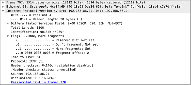
Figure 2-6   Fragmented IP message

Once you have fragmented a message, you need to know how to put it together again. First is the offset field, which you can see in Figure 2-6. This tells the receiving system what byte to start this set of data at. If you have bytes 0–1450 in one message, the next message is going to start with byte 1451, which will be the offset for the second message. If there are 1000 bytes in that message, the third message will start at an offset of 1551 (1451–1550 is 1000 bytes). However, in order to begin putting all these messages together, we need to know how they go together. This is done with the IP identification field. All frames that have the same IP identification value belong together. If there are no fragments, the IP identification field isn’t used at all.

The IP header also includes the version number, which you will commonly see as either 4 or 6, with 4 still being more widely used. You will also see a value indicating how long the IP header is. If you look closely at a packet, you might see a value of 5 in this field of an IPv4 packet. This is because the field captures the number of 32-bit words in the header. The header size has to be a multiple of 32 bits. In the case of a value of 5, that means we have 5 times 4 or 20 bytes. The 4 comes from the number of bytes in a 32-bit word. The IP header provides an indication of what protocol should be expected next. In the case of Figure 2-6, it’s ICMP, which is the Internet Control Message Protocol.

Finally, we have the source and destination address fields. This packet is IPv4, which means there are 4 bytes in the address. A byte has a potential range of values of 0–255 and an address is delimited with dots between the individual values. This doesn’t mean, though, that you would have any value in those values.

IP Addressing

While you may not see it a lot, since people tend to use hostnames, the IP address is foundational. They are also, often, not entirely understood when it comes to how they are put together and, more importantly, how they are collected. We’ll talk about how the addresses are subnetted in the next section. The addresses, though, look straightforward. Not all addresses are the same, though. First, unlike MAC addresses, IP addresses are collected. They come in groups. The groups are called networks, and part of the IP address is the network part. The other part of the IP address is the host part. You’ll see how these two parts are identified just ahead.

IPv4 In the early days, IP networks were divided into classes. There are five address classes from A to E. This isn’t a class in the sense of social class, meaning one class is better or has more privileges than others. The class in this sense has to do with the size of the block of addresses that are available to each class. When it comes to IP addresses, it’s best to think about the binary representation, since it will help with the addressing as well as, later on, identifying the network portion of the address. Table 2-1 shows the sizes of the IP networks according to the classes as well as how to identify which class an address belongs to. Once we have identified the IP networks, we can talk about some of the special networks.

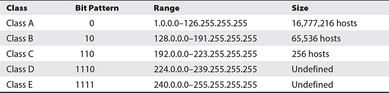
Table 2-1   IP Networks

When you take the binary representation of the first octet, you can determine which class an address belongs to based on the bit pattern of the most significant bits in the first octet. As an example, 110.55.10.0 is a Class A address. The bit pattern in the first octet is 0110 1110. Because the most significant bit is a 0, we know it’s a Class A. More importantly, understanding binary arithmetic will let you know where things are. Class A addresses go up to 126 (technically 127, but we’ll get into that later). This can be seen with a little binary arithmetic since the most significant bit is the 2^7 place. 2^7 is 128. Since there is always a 0 in the 2^7 place, no Class A IP can be larger than 128.

Think about it this way, in case binary isn’t a natural arithmetic language for you. Let’s say that Class A addresses are anything below 1000. The most significant bit in this case is 10^3, which is 1000. You can’t reach 1000 without a value in that position. The largest value we can get is 999. The same is true in binary. The largest value we can get without that 2^7 place is 127. Once we hit 2^7, we are at 128, but we can’t get there with a 0 in that first position. This is why the bit pattern in the other classes indicates a 0 to terminate the pattern. A 0 in the second most significant bit means we never catch the 2^6, which is 64. This means we can never get to 2^7 + 2^6, which is 192. The highest we can get to is 191. Since we have to have a 1 in the most significant bit position, we start at 128.

There are special addresses that you should be aware of. The first, since it came up already, is the address block 127.0.0.0-127.255.255.255. This is an address block that has been marked for use as a loopback address. A loopback address is generally used to refer to the system that owns the address. If you send a message to a loopback address, it returns to the system that originated the message. This is not hard-coded, however. It’s a convention rather than something set in stone. You are perhaps familiar with 127.0.0.1, because it’s commonly used as the loopback address but every address in the 127 range can be used as a loopback address.

You’ll see Class D and Class E addresses in Table 2-1. Class D addresses are all used for multicast. Multicast means you are sending a message to a group of systems rather than an individual system, which would be unicast and the most common. Class E addresses are considered reserved. They were left for experimental purposes and for potential future needs.

Also by convention, there are address blocks that are used for something called private addressing. You will hear these referred to as nonroutable addresses, which is misleading. They are nonroutable across the Internet by convention, as defined in a document called Request for Comments (RFC) 1918. It doesn’t mean they are never routable. If you have a large network, you can route these addresses inside your network. You can’t, though, route any traffic to these addresses to any other network across the open Internet. You may also want to reread that last sentence. Notice what it says to those addresses. You can have one of those addresses in as a source because routing isn’t based on source, it’s based on destination.

The private addresses are ones you may already be familiar with and they were created based on address classes. The Class A address block is 10.0.0.0–10.255.255.255. The Class B address block is 172.16.0.0–172.31.255.255. The Class C address block is 192.168.0.0–192.168.255.255. If you have a home network and a modem from your Internet service provider that hands out IP addresses, you are likely familiar with one of these address blocks. A commonly used block is 192.168.0.0 or even 192.168.1.0. These larger blocks are broken into smaller blocks. After all, you don’t need 65,536 hosts on your home network. In reality, it’s likely you only need 10–20, perhaps. Unless you are loaded with technology from basement to attic. In which case, maybe 100–150 on the top side. Even that’s smaller than the 256 of a Class C address. This is why we don’t use classes anymore.

IPv6 We have run out of IPv4 addresses. At least, that’s what we’ve been hearing for the last several years. In fairness, it’s a cascading thing. The Internet Corporation for Assigned Names and Numbers (ICANN) has a function called the Internet Assigned Numbers Authority (IANA), responsible for doling out IP address blocks. Initially, ages ago, entire Class A address blocks were handed out to large corporations like IBM and General Electric. These larger blocks have long since been broken up into smaller network blocks and handed out to various regional Internet registries (RIRs), responsible for handing out the addresses to organizations within their region. IANA has apparently handed out the last block of addresses it has to hand out (in reality, this has happened on more than one occasion as they find more blocks that can be freed and distributed). That doesn’t mean that all the RIRs have handed out the last network blocks they have to give out. Once they have handed out the last blocks, the Internet service providers who are likely the ones getting them will still have network blocks to give out to their subscribers. As I said, it’s a cascading thing.

This is important because the lack of address space in IPv4 triggered, in part, the need for IPv6 more than two decades ago. Along with several other improvements to the overall functioning of the protocol, IPv6 uses a much larger address space. Instead of 32 bits for network addresses, IPv6 uses 128 bits. This has caused the way we represent addresses to change. An IPv6 address with 128 bits would have 16 decimal addresses to represent. That’s potentially 48 numbers, which doesn’t include the dots in between them. Very unwieldy for writing or communicating. Instead of using a decimal representation, IPv6 has moved to a hexadecimal representation of the values of the address. This is convenient because every byte can be represented as two hexadecimal digits. The maximum value of a byte is 255, which is ff in hexadecimal.

Rather than dots separating the components, we use the : (colon) in IPv6. The address is segmented into blocks of four hexadecimal digits, which is 2 bytes. You don’t have to use every single digit, though. If there are any leading 0’s in a block, you can omit them. Additionally, if there are blocks that are all 0’s, you can omit the entire block and just make sure you use a double : to indicate there is a missing block of digits there. As an example, the loopback address in IPv6 is represented as ::1. This means there are all 0’s in the address except for the least significant digit in the last byte. If you have an unspecified (blank) address, with all 0’s, it is represented as ::.

An IPv6 address has well-defined elements. Where subnets in IPv4 rely on an extra piece of information, in IPv6 the address has the network identifier built into the first half of the address. The first 64 bits of an IPv6 address identify the network, including 48 bits or more of routing prefix and up to 16 bits of subnet identifier. The second half of the address identifies the network interface. Note that this doesn’t say it identifies the system because each system may have multiple interfaces. This portion of the IPv6 address may be the MAC address for the interface, which would uniquely identify it on the network. This is not the only way an IPv6 is composed. Your network may have a Dynamic Host Configuration Protocol 6 (DHCP6) server to hand out interface identifiers. The identifier component may also be assigned randomly or manually.

Subnetting

We don’t use classes anymore in the sense of how we break up networks into separate entities. However, we still use networks. How do we handle networks then? Well, first, we should talk about why we use networks or subnets. We have to have a way to break the entire collection of systems into smaller groups to make communication manageable. We can’t switch every device on the Internet, so we have to make use of a higher layer protocol. Systems need to know where to deliver messages to, which is why we use subnets. Your system will make a determination about whether the destination address is on your local network, based on the destination address as well as the IP configuration on your system. You can see an example of a network configuration from a Linux system below.

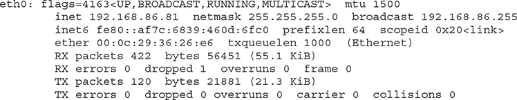
Along with the IP address, you can see the subnet mask, referred to as netmask. The netmask is how your system determines which part of the address is network and which is host. We’re going to go back to binary for this so you can understand how the masking works. In the example above, the network mask is 255.255.255.0. The IP address is 192.168.86.81. In order to get the network portion, we use the logical operator AND using the IP address and the network mask. You can see how this works below using the binary representation of each octet.

The logical AND requires that both values be 1. The host portion of the network mask is all 0’s, so it will mask to all 0’s against the IP address. You can try this with any network mask you would like and you will get the network address associated with the IP address back. It may be worth looking at different network sizes at this point since we’re looking at clean boundaries so far that align at the byte. It’s helpful to know what it looks like when your boundaries are not aligned with the byte, meaning we have some bits but not all bits in one of the bytes of the network mask being used.

Another way to think about the network mask is to count the number of bits in the network mask. Each byte has 8 bits so a subnet mask of 255.255.255.0 has a total of 8 × 3 bits or 24 bits. When we use the number of bits to designate the network mask, we are using Classless Interdomain Routing (CIDR, pronounced cider) notation once we append the number of bits to the network, as in 192.168.86.0/24. When you start thinking about the number of bits, it may help you understand developing subnets better. Adding a bit to the network mask gives us a total of 25 bits. Since we are using one bit in the last octet, the binary representation looks like this: 11111111 11111111 11111111 10000000. Keep in mind that the most significant bit has a value of 128. This means the subnet mask is 255.255.255.128. Adding another bit gives us CIDR notation of 265 and the last octet looks like this 11000000, which is the same as 128 + 64 (2^7 + 2^6). Every time you add or subtract a bit, you are adding or subtracting a power of 2.

The same thing happens in the opposite direction. If we go from 24 bits of subnet to 23 bits, the third octet looks like this: 11111110. The least significant bit has a value of 1 (2^0). When we subtract it from the maximum value of a full byte, we get 255 − 1 = 254. The network mask in that case is 255.255.254.0. Losing another bit of subnet, we subtract 2 from the previous value (2^1). This leaves us with a subnet mask of 255.255.252.0.

Every time we adjust the subnet mask, we either gain or lose in the total number of hosts we can have on the network. If we add a bit to the network mask, we have to lose a bit from host portion. Every time we add or lose a bit, we multiply or divide by 2. Since we are losing a bit, we divide by 2. The total number of addresses with a subnet mask of 255.255.255.0 is 256 (0–255). If we lose a bit, we have a total number of hosts possible of 128. We also change the parameters of the network. The 192.168.86.0 network has a range of 192.168.86.0–127. Out of the original network, we now have a second network that also has 128 potential addresses—128–255. Imagine you are cutting a pie into halves, which you can see in Figure 2-7. Our original pie of 256 addresses becomes two halves, each with 128 addresses.

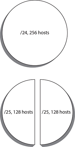
Figure 2-7   Pie diagrams of subnets

If we added another bit of network, we’d have four networks out of the original network that has 24 bits of network mask. The ranges would be 0–63, 64–127, 128–191, and 192–255. Our pie becomes quartered at that point. If you want to break it again, you will have eight slices of pie that each has 32 addresses. Keep in mind that you are working with adding and subtracting bits when you are subnetting so you will always have a power of 2 when it comes to numbers of network segments and numbers of hosts. You can’t, for instance, break your network into six subnetworks. It has to be eight if you need six, which means you’ll have two that are leftover. Think binary. It will help you.

These calculations are made when systems try to communicate to an IP address. If the system you are trying to communicate with is found to be in your network range, your system will send the message directly to the MAC address. Otherwise, the message needs to pass through a layer 3 device, meaning it has to be routed off your network and to a different network. That means your system will send the message to the MAC address for the gateway that will get the message to the destination host. Any device that passes a message from one IP network to another IP network is called a router, because it is routing messages, rather than simply switching or forwarding them.

Routing

Routers forward messages from one network to another network. You probably use them every day. When they are working, you aren’t even aware they are there. When they aren’t, it’s a problem. Before we get into more complex types of routing, we should look at a routing table. Every networked device has a routing table. It keeps track of destination networks and how to get to them. Endpoints have a simple routing table, as a general rule. You can see an example of a routing table below. It shows the target networks, the network mask for that target network, the gateway device that messages destined for that network should be sent to, and the interface the message should be sent out. This is important because you might have multiple interfaces that can get to the same networks.

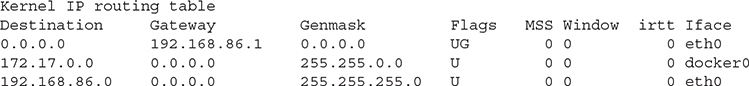
The one special case above is where the destination is 0.0.0.0/0.0.0.0. This is a wildcard, meaning any network that doesn’t have a specific match should be sent to the gateway for this address. The device you are sending to is referred to as a default gateway because it’s the device all traffic defaults to if there is no specific place to send the message. In most cases, you will have two routes if you are looking at the IPv4 routing table. You’ll have the route to your local network, which should indicate the message should just be sent out the local interface. You’ll also have the default route. In the case shown above, there is a separate interface attached to the system. This interface has its own IP address, which is on another network altogether. That means there has to be a route entry for that network. Of course, you can also get the IPv6 routing table as well. It’s a little more complicated, and you can see it below.

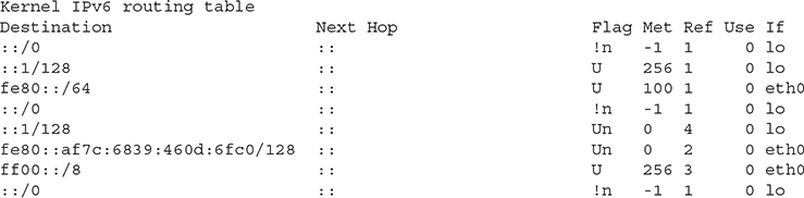
You’ll see fe80 in your IPv6 routing table. This is referred to as a link local address that identifies a physical link and may be used for the neighbor discovery protocol (NDP). The NDP is used to gather information from the network to automatically configure your device. This includes identifying gateways on the network so you know where to send packets, based on the destination addresses served by the gateway.

When you are setting up a lab, you may have cases where you want to have multiple IP networks. This means you will have to have a way to route traffic from one network to another. This is not something that can be done with a switch, since a switch is only for passing traffic within the same network, using layer 2 addresses (apologies for the repetition, but it’s an important point that bears repeating). Before you think about the devices you are going to use, we can talk about the different types of routing. The first is static routing. This is where you enter all the routes in by hand and just make use of the routing table and capabilities with your system.

You can see an example below, where a static route entry is added to the routing table on a macOS system. Once the route entry has been added, you can see the change in the routing table. What the route add statement does is it tells my system that if there are any messages that need to go to the network 172.30.42.0/24 (meaning, 172.30.42.0–255), they should be sent to the gateway at the IP address 192.168.86.250. You will note from the routing table that the primary or default gateway is 192.168.86.1. The IP address 192.168.86.250 is on the same subnet. You can’t have a gateway that is on a different subnet than the one you are on because the communication will happen over layer 2. The whole point of a gateway is it handles the layer 3 movement.

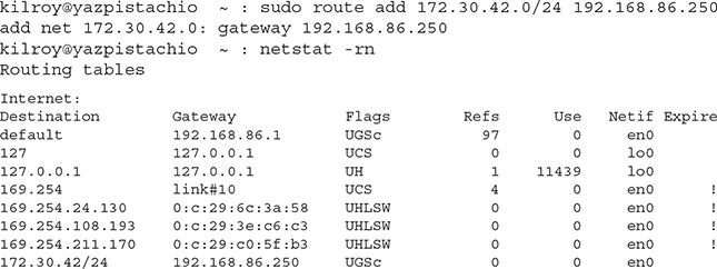
Static routing is cumbersome, though. It’s fine if you have a very small number of systems and network routes. If, for example, I had a test network on 172.30.42.0/24 and I only wanted to get to it from a couple of systems on my local network, it would be fine to use static routing. I just have to add the routes to those systems and everything would be okay. It requires a router be at 192.168.86.250 and that router has to know how to get to any other network so devices behind it can get around. In other words, you have to design how your traffic is going to flow and enter it into the routing tables that matter.

This is not ideal, however. While it would work well for a small number of networks and systems, it doesn’t work well in cases where there are a lot of systems or networks. It also doesn’t work if there are a lot of changes to the network. When you have a lot of changes to the network, you really need to make use of a dynamic routing protocol. The administrative overhead without that is cumbersome. Once you add in a lot of administrative overhead that relies on manual work, there is the potential for error and misconfiguration, which means things don’t work, which means time in troubleshooting to find where the thing that doesn’t work is, which means fixing it and hoping you don’t introduce more errors which means … whew. It seems easier to just use a dynamic routing protocol.

Link State Routing Imagine that you kept a map of the entire network around in your head and you always know exactly the best path from one node on the network to another because you can calculate it based on comparing all the different paths possible. Take a look at the map in Figure 2-8. You want to get from node A to node G. If you step back and look at the map in its entirety, you will see that there are the following paths to get from A to G: A-D-C-F-G, A-B-E-F-G, A-B-C-F-G, and A-E-F-G. All else being equal, the path that is the best is A-E-F-G because it has the fewest intermediate steps.

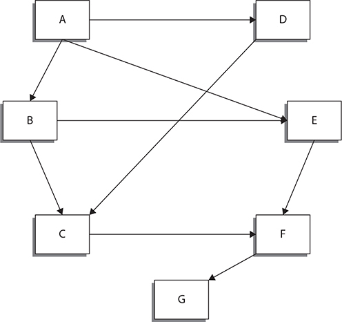
Figure 2-8   Network map

With a link state routing protocol, every node in the network sends out information to every other node in the network. What it tells them is who the node is and what other nodes it is directly connected to. This may be the name of a node, meaning a routing device, or it may be the identification information for networks that are directly connected. Every node can then construct a map of the entire network from those pieces of information. Since networks may be constantly in flux based on nodes that are connected or disconnected or other changes, this map would also be in constant flux. In order to address that, along with the link state advertisement, there will be a serial number to identify which version of the link state advertisement is being sent. A more recent serial number would carry more weight than an older one since it would be considered more up-to-date and, likely, more accurate as a result.

Link state protocols use some variant of Dijkstra’s algorithm. You may be most familiar with the use of Dijkstra’s algorithm from your car. Your navigation system more than likely uses an implementation of Dijkstra’s algorithm. In the case of a network routing table, there is a link cost, much like there would be for a road you might take. The link cost on a network may factor in parameters like the amount of bandwidth on any given link. A link with more available bandwidth would have a lower link cost than one with less bandwidth. The same would be true on roadways. If you have a choice between a road where the average speed limit is 60 and a road where the average speed limit is 50, you’re probably going to take the road where the average speed limit is 60, assuming the distances are roughly comparable. This cost is factored into decisions about which path to take.

There are two common link state routing protocols. The first is called Open Shortest Path First (OSPF). This is a very common routing protocol, used in large organizations. It uses the concept of areas within an autonomous system to assist in making decisions about which paths to take from one point to another. This makes it an interior gateway protocol, meaning it is used to route within a single large network rather than between unrelated networks. A single organization is an autonomous system, which may have any number of subnets. While the organization is autonomous, meaning it relies on itself, it does need to have a way to get from one network to another within the autonomous system.

Another type of link state routing protocol is Intermediate System to Intermediate System (IS-IS). IS-IS was designed to run at layer 2, which means it is not as tied to IP as OSPF is. It also uses Dijkstra’s algorithm to make decisions and has the concept of areas, though it defines them differently than OSPF does. IS-IS is also an interior gateway protocol, and it is perhaps most commonly used as a routing protocol within the backbone of large service providers.

Distance Vector Routing Network routes generally rely on three properties. The first is the route itself, meaning the networks that can be reached through the next hop interface, which is the second property. In the routing table you saw above, the interface is the last column on the right. The first column on the left is the route entry, telling us what networks or systems can be reached through the route entry. The last property in a routing table is the cost. If you have two route entries for the same network route, you need to have some sort of cost associated with each route. We saw this a little earlier when we looked at the different paths through the network map in Figure 2-8. Distance vector protocols make use of this because they count the number of hops (intermediate network devices/routers) in a path.

Take a look at Figure 2-9 now. You’ll see it is the same as Figure 2-8 with the exception of the addition of network costs. This is the one piece missing from the previous map. In order to use a distance vector protocol, we need more than just the path (vector). We also need the distance (cost). These costs can be calculated in multiple ways and can often be hand-configured for traffic shaping. The cost of a vector or path may be literally a cost, meaning there may be a dollar value associated with it. You may have one path that has 10 times the bandwidth but maybe it costs 20 more per bit than another path. In order to keep your financial costs lower, you may prefer to only use the higher bandwidth link as a backup rather than the primary link.

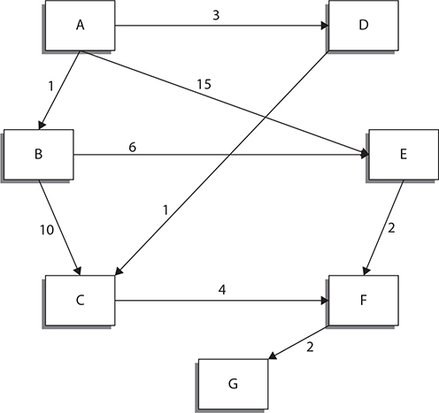
Figure 2-9   Distance vector map

Now, let’s take the same paths we had before and start looking at the actual costs of those paths, giving us both distance as well as the vector.

According to Table 2-2, the best path is now no longer A-E-F-G. That ends up being the highest cost path. The best path is now A-D-C-F-G, followed very closely by A-B-E-F-G. What seems like the shortest path is actually the path with the highest cost, though just based on this information, we can’t be certain why it’s the highest cost. For whatever reason, the “short cut” from A to E ends up being really expensive.

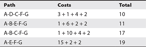
Table 2-2   Distance Vector Costs

There are a number of distance vector protocols that are in use. Perhaps the most common is the one that is used to route traffic across the Internet from one autonomous system to another. This is the Border Gateway Protocol (BGP). It is an exterior gateway protocol because it routes from one autonomous system to another. Of course, BGP does come in two different variants. One is an interior gateway protocol, referred to as IBGP. The exterior gateway protocol is EBGP. EBGP is probably the flavor of BGP most commonly thought of when you just talk about BGP.

The oldest routing protocol in use is also a distance vector protocol, known as the Routing Information Protocol (RIP). RIP is a very simple routing protocol because all it used was the number of hops from one node to another. It didn’t matter how much bandwidth each hop had available or even how far the hop is. As far as RIP version 1 was concerned, a transcontinental link from Los Angeles to Boston was the same as a link from San Jose to San Francisco. A hop is a hop is a hop after all. A limitation to RIP is the size of the network it can support. RIP can only support up to 15 hops between a source and a destination. Because of that and many other limitations, RIP is not widely used. It can be, however, a choice for an easy-to-implement routing protocol on smaller networks. It is dynamic and there are software packages that can be easily installed and configured to manage routing on networks.

Network Topologies

There are a number of network topologies that can be used, though in fairness, there are really only a couple that you’re going to be most likely to use in a local area network. The first, and most common today, is a star topology. The star topology is used in Ethernet installations because there is a single network device at the center of the network that manages all the connections to other devices. Today, this is generally a switch, though you may also use a hub. Hubs are harder to come by today, and they have none of the advantages of switches. You can see an example of several computers connected to a switch in a star topology in Figure 2-10. Many people use Wi-Fi networks today. These are also star networks because there is a network access point in the “center” of the network. All stations on the network communicate to the access point, which communicates with the other stations in turn.

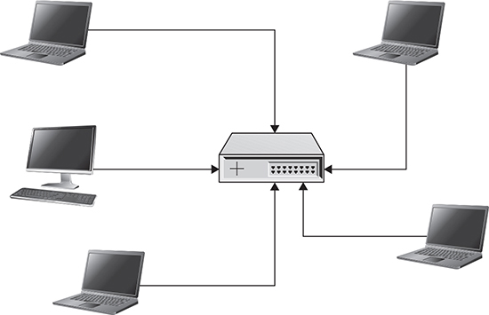
Figure 2-10   Star topology

Another topology, less likely to be seen but still worth talking about, is the bus. A bus topology is where you have one long cable, essentially, that everyone connects to. A common bus implementation may have had a long coaxial cable that everyone connected to by using taps that tapped into the copper cabling. This is not the only type of bus implementation, of course, but it was a very common implementation of a bus network for a very long time. You can see an example of a bus topology in Figure 2-11.

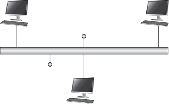
Figure 2-11   Bus topology

The reason it’s useful to talk about a bus network is what is more common today is a hybrid of a star and a bus. In even many modern homes, you may be forced to use a star-bus hybrid network simply because, if you are like me, you still like having wired connections because they are generally faster and potentially more reliable. Modern homes, at least the ones I am used to, having been through a few different ones in the last couple of decades, have a small number of ports that run back to a box in the basement. You probably don’t even have a patch bay, where you can plug either Ethernet cables in or maybe phone cables, if you prefer to use a phone in a given location. Instead, you may have just raw Cat5 or Cat6 cables to plug directly into a switch. What this means, though, is you probably need to have small switches in rooms where you want to plug in multiple network devices.

As an example, let’s say you have a smart TV, a gaming system like an Xbox, a streaming device like a Roku or FireStick. All of these can have wired connections. You only have one port near the TV but you have at least three cables you want to plug in. This means you need to have a small switch there. The moment you connect two switches together, you have a star-bus hybrid network. The reason is you have multiple stars (the switches that all your systems connect to) and then you have a bus that connects your stars together. You don’t have a single star simply because you have at least two centers. A star doesn’t have multiple centers (you have to imagine a star in this context a bit like a jack, the toy you played jacks with, where you have a small center and arms radiating out from that central nexus).

Design Requirements

Your design is going to be driven by requirements. If, on the off chance you are performing testing on Synchronous Optical Network (SONET) devices, you may end up needing to implement a ring topology. A ring topology is just like what it sounds like—all the devices are connected to network cabling that looped back on itself, meaning it forms a ring. The ring means that you toss a message out onto the ring and it just circles around until it reaches its destination. You don’t have switching where a device sends the message out a port to an attached system. You just toss it out to the ring and it loops around. This is just one example where the type of testing or the devices you are testing with will drive how you design your network.

Cost is often significant factor. Most of us don’t have deep pockets to splash out on a lot of networking equipment. You may not have the ability to have a lot of physical devices, for instance. You may be forced to use all virtual systems, which means you will have limited choices when it comes to your topology. A desktop virtual machine setup is going to behave as though you have a single device on its own subnet with a gateway device, which the virtual machine software takes care of. Some virtual machines will give you more flexibility, but for the most part you are probably looking at making use of a star topology because you will be given a virtual switch to connect to.

Understanding the objectives of your testing will help you to design a network that will support those objectives. Always know the objectives before you start out with your network design. This is akin to understanding the problem before you start working on a solution. If you haven’t defined the problem, how can you know if the solution actually solves the problem? The same is true for designing your network. How can you know if the network will support the goals of your testing if you haven’t clearly identified the goals of your testing? There are cases where you will have to have physical machines to test with because you have a hardware device that needs to be part of the testing. If you’ve built a virtual lab with nothing but virtual machines, you won’t be able to achieve the ultimate objectives for your testing.

This is where documentation may be helpful. Start out by clearly making a list of what you want to accomplish. Even if what you want to accomplish is just to learn an operating environment like Parrot OS or Kali Linux or Command VM better. Write that down. Write down what you need to accomplish that objective. For a start, you need a place to install the operating system. You also need at least one target to practice against. If you are simply learning how to scan better, with all the different types of scans and capabilities of scanning tools, you still need at least one target. You may not be able to scan your own system and get useful responses.

Write down your objectives and make your list of requirements. From there, you can determine the systems that you need and any other hardware you may need. Once you have all of that in place, you can start designing your lab network and placing your systems into correct positions based on the overall requirements.

The Importance of Isolation

When you are security testing, one important idea to keep in mind is that what you are doing is illegal, or at least can be illegal. You’ll hear this idea repeated over and over again, because it bears repeating. If they are not your systems you are testing against, you can find yourself in a lot of trouble. Well, perhaps not a lot of trouble in reality but the potential is there because most everything you may be doing related to security testing is a violation of the United States Computer Fraud and Abuse Act (18 U.S. Code § 1030). That’s just in the United States. Other countries have similar and sometimes stiffer laws protecting against the unauthorized use of computers. This is not to scare you or tell you security testing is a bad idea. It’s intended to convey the reality of the landscape you are walking into. It’s also intended as a preamble to the idea of isolation.

Most people aren’t intending to do ill when they start security testing. Sometimes they are just trying some things out. Unfortunately, and this is a very old lesson, things can get out of hand very quickly if you aren’t careful. Robert T. Morris, more than 30 years ago now, was doing some testing (or at least this was his defense when the case came to trial) and a piece of software he was working on got away from him. Literally got away from him, meaning it traveled off the system he was working on and started spreading to every Internet-connected system it could find. This was more than 30 years ago, so there was only a fraction of the total number of systems out there than there are today. However, where today we have primarily small, reasonably inexpensive systems, then the systems that were connected were million dollar plus systems. Morris wrote a piece of self-replicating software to test against repairs of known vulnerabilities.

Let’s take him at his word and believe it was always meant as an exercise that was to be contained within his own system. Even with the best controls in place on the system you are working on, it’s hard to say whether what you are doing will end up squeaking out onto the greater network, causing damage you didn’t expect. This is why isolating your testing networks is such a good idea. There are a few different ways you can perform this isolation.

Air Gaps

An air gap is where there is a space of air between your system and the rest of the network. What it means effectively is your system or systems are not connected to anything else. You may do this in the physical world by connecting all your systems to a single switch and nothing else. You don’t connect to a modem/router. You don’t connect to any other switch. You connect everything that needs to talk on the network to one switch. That’s air gapping. You can achieve the same sort of thing in virtual machines by putting everything onto a virtual switch that is not connected to anything else. It has no way to get to anywhere other than the single broadcast domain that the systems attached to the switch are connected to.

If you are working on a larger environment, you can still achieve the same air gapping. You can have multiple network segments and multiple routers if you need to. The one thing you do not have is a connection to anything outside of the space you are working in. Let’s say, for instance, that you have a room where all of your lab equipment is. You may have multiple racks with multiple servers. You may have multiple switches. This is all fine, as long as you never connect anything in that room to anything outside the room. You leave out the uplink, as it were. This means your systems in the lab room can communicate with each other and you may even be routing between subnets. You are simply not connecting to anything outside of your lab room.

Routing

Remember that we have switching and we have routing. Switching happens at layer 2 with MAC addresses. You may have a single subnet with all of your systems on a single broadcast domain. Once we cross over into another subnet, we pass a layer 3 boundary. This requires routing, but it also requires that you have a router to pass the traffic from one network to another network. What if you didn’t have a gateway configured on your system. Take a look at Figure 2-12. You can see a couple of systems connected to a switch. The switch is connected to a router. The only thing that makes that router usable is a configuration setting telling the operating system where to forward messages that belong to another network. Without that configuration setting, nothing goes off the local network.

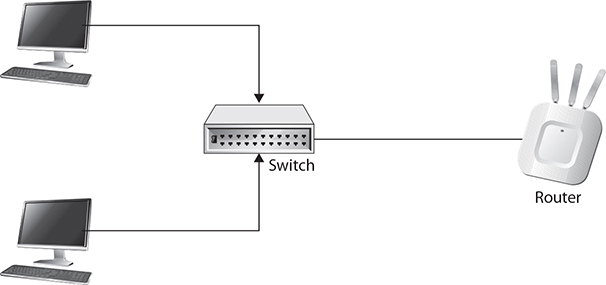
Figure 2-12   Small network with router

Just because the router is there doesn’t mean it needs to be used. Of course, the default gateway is often configured automatically through the dynamic host configuration protocol (DHCP). The way around this is to use manual configuration on your systems and just leave the default gateway out of the configuration. Even if the system complains about not having one, you will have protected other networks from anything you may be doing.

If you have some more hardcore routing chops, you could black hole routes. This means that you create a route entry for any networks and provide a nonexistent address for the gateway. In Unix terms, you are sending all the traffic for that route to /dev/null. You could also call it sinkholing the traffic. Either way, you are taking traffic on the network and send it to a location where it doesn’t ever go anywhere useful and nothing ever returns. Because you need to pass network traffic across a layer 3 gateway to get the traffic anywhere outside of your local network, manipulating the route tables can prevent the traffic from getting anywhere outside of your local network.

Firewalls

A firewall is a device that makes decisions about what traffic to pass across an interface. A network firewall forwards messages from one interface to another based on routing tables, which makes it a de facto router. It’s not the ability to forward from one interface to another interface that we are interested in here. It’s the ability of a firewall to make decisions about what traffic to pass from one interface to another and what traffic not to pass. Below, you can see an example of the use of a Linux firewall, iptables, to block traffic from our network to a couple of destination networks. This is a little backwards from what you usually expect to see. Normally, we would be blocking on the INPUT chain, not the OUTPUT chain, because usually we are trying to protect our systems from those people on the outside. However, the capability does exist within iptables, and any other firewall.

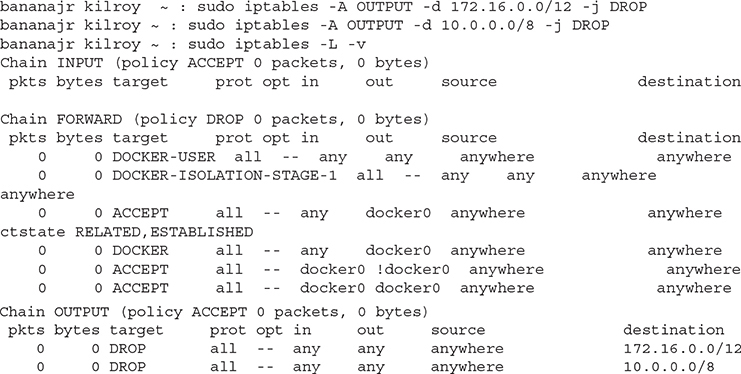
There is one thing to note in the action, which is what follows the -j in the iptables command. You have multiple choices for actions but the two we are going to be most interested in for this application is DROP or REJECT. If you were to REJECT a packet passing through the firewall, you would be following the standards for the protocols. This means either sending a TCP RST or an ICMP unreachable error message. This is polite, meaning you are telling the sending system what is happening so it can recover gracefully from the attempt. A DROP, however, means the firewall just drops the message without worrying at all about letting the sending system know what has happened.

These firewall rules were on a system with a single interface. This means that there is no input interface or output interface. We could indicate which interface we were blocking the output on, if we had multiple interfaces. In this case, there is only a single interface so we don’t care about what the INPUT versus OUTPUT interface is. There is only one interface that leaves the system. By the way, you can use host-based firewalls to protect everything outside of your testing system and system under test. You let traffic out to the IP addresses you are working with and block everything else. This does mean, though, that you need to be aware of order of operations. You can’t have your block rules before your allow rules if your firewall is a match first rather than match best. A match best firewall would see a more specific rule since you are being specific about IP addresses you are letting in. Your block rules are going to be broader—either you are blocking everything or else you are blocking only specific network blocks.

I don’t want you to think that you have to be using Linux systems to be able to use host-based firewalls. You can use Windows systems. The Windows firewall was introduced in Windows XP Service Pack 2, which means it would be very unusual for you not to have it if you are running Windows systems. Ideally, you aren’t still using systems that are over 15 years old. It is currently called the Windows Defender Firewall and you can get access to it from the Settings page/applet. In order to do things like block entire network ranges, which you can see part of in Figure 2-13, you would need to get to the advanced settings. In the basic settings, you can block individual applications since the firewall is based on monitoring the behavior of specific applications. Of course, if you are most concerned about one application over others, you can use the basic functionality of the Windows firewall to just block traffic from that application.

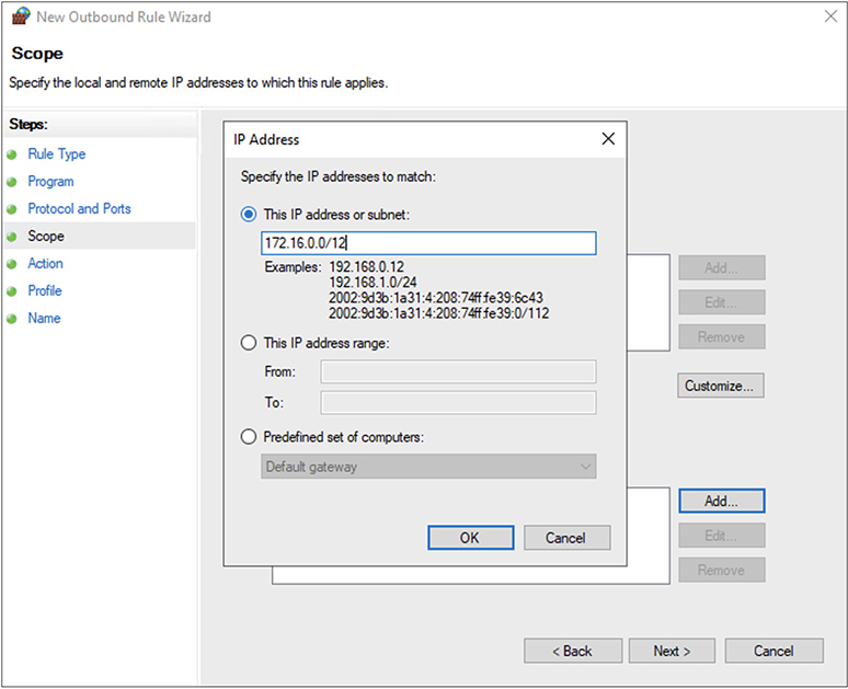
Figure 2-13   Windows Defender Firewall

Configuring the firewall uses a wizard-style process, which is why you can’t see all the configuration settings in Figure 2-13. You can only see adding an IP address. Along the left-hand side of the dialog box, though, you will see the process that gets followed. You can get very granular in the firewall. If you just want to allow some traffic while blocking the rest, you could create rules in the Windows Defender Firewall.

These are, of course, just a couple of examples of firewall usage to block traffic from impacting other systems and networks. They are not the only ways of approaching the problem of ensuring your activities don’t impact others. If you had an actual router, for instance, like an older Cisco for instance, that you are using in your lab (older because we’re talking about a lab on the cheap and newer ones are considerably more expensive), you could use access control lists to make simple determinations about permitting or denying traffic. These are less feature-rich and robust than firewalls and firewall rules are, but they would work if you wanted to block large amounts of traffic based on destination address blocks.

So, no matter what approach you use, whether it’s simple access control lists, host-based firewalls or complete network-based firewalls with multiple interfaces, you have the ability to block traffic from having a negative impact. One issue to consider, though, is misconfiguration. You want to double check your configuration before doing any testing that could get out of hand. Have a second set of eyes look at it. This is especially useful if you are using complex rules. A couple of extra minutes looking over rules that are in place and even testing the rule to make sure it actually blocks will be far better than knocking over someone’s production system (even if it’s yours).

Summary

While many people talk about the Open Systems Interconnection (OSI) model when it comes to identifying layers of functionality in network communications, there is a better than good chance you are using TCP/IP so it’s best to understand that architecture for our purposes. First there is the network access layer, which provides not only the physical connection but also addressing in the form of the MAC address. This is the address that gets used within the local subnet, on the broadcast domain. If you have moved beyond the local subnet into another network altogether, you have passed up the stack into the internetworking layer. This is where IP reigns and the IP address is used to move traffic from one system to another.

Once we hit the internetworking layer, we have to talk about how to break up IP networks into manageable chunks. These are called subnets. When you are creating subnets, it’s important to keep in mind that every IP address has two components—the network portion and the host portion. You would determine which is which by using the subnet mask in IPv4. This is another dotted quad, like the IP address is. Every bit that has a 1 turned on in the subnet mask is a bit that is part of the network address in the IP address. You use a logical AND against the IP address with the subnet mask and you’ll get the network address out.

It’s helpful to keep binary in mind when you are creating subnets. Every bit of subnet mask you use changes the number of hosts available by a factor of two. If you add 1 bit of subnet mask to what’s in place, you end up with two networks from the original network block while simultaneously cutting the size of each block in half. If you subtract a bit of subnet mask, you will end up doubling the number of IP addresses in the network block. Notice, I used IP addresses and not hosts. This is because every network, no matter what size, has to have a network address and a broadcast address if it is going to be useful at all. When you split a network in two, you have twice as many network addresses and broadcast addresses. Because of that, you aren’t halving the hosts. You’re actually halving and then subtracting 1. So, if you start off with 256 addresses, only 254 are useable, you would halve to 128, of which 126 were useable. Half of 254 is 127, but we have to accommodate for the additional overhead IP address, so we subtract 1, giving us 126.

Commonly, you are going to use a star-bus or maybe even a star network topology. It’s possible that you could use a ring or maybe a bus, but they are less common unless you are developing wide area networks, in which case rings are far more common. In fact, the Internet as a whole is something called a mesh, which means nodes (border routers) are connected directly to one another without going through a central access point. And because they are essentially haphazard, it’s not a bus. Nothing is connected completely in sequence.

I am a firm believer in identifying the problem before you start working on the solution. A solution in search of a problem is not something you really want to have. Make sure you understand the problem and your objectives. You can work on writing them out, which can be very beneficial, so you have them in black and white (or whatever other two colors you prefer) in front of you. This helps later on when you need to go back and make sure you have adequately addressed the issues in the requirements with the network design you have selected. Networks can become complex, and this is especially true if you are trying to mimic the production network you are trying to test. You may have multiple subnets connected together with multiple intermediate systems. Being able to go back and check against your requirements is useful. So, document your understanding of your objectives and requirements.

Isolate your systems. Keep in mind that very often, what you are doing is illegal. There are laws against unauthorized computer usage. Even if you didn’t mean to affect another system, sometimes overspray can hit other systems and have negative impacts to them. As a result, isolate them. You can use air gaps, meaning you have completely isolated them because there is no cable or wireless connection leading from your testing environment to any other network segment. You could also use routing. You may black hole routes, meaning you send traffic into oblivion with entries in your routing table. You can also use firewalls to block traffic outbound from your network to other networks. As always, before you do any of your actual testing, make sure your isolation controls are functional.

In the next chapter, we are going to start putting some of these ideas into practice by looking at ways we can create systems to test with or test against. One of the most cost-effective ways to do this is to make use of virtual machines, so we’re going to talk a lot about virtual machines, with a little comparison with physical systems thrown in for good measure.