 CHAPTER 8
Someone Has to Win
Betting against Expectation
The probable is that which for the most part happens.
—Aristotle, Rhetoric
Play a game of chance, any game of chance. It could be flipping a coin, shooting craps, playing roulette, or betting on a horse race. In the end you either lose or win. Let us introduce some notation: P(A) will represent the probability that event A will turn out successfully. For example, if W represents a win and L a loss, then P(W) is the probability that you win your chosen game and P(L) the probability that you lose. If you were flipping a coin, then P(W) would equal 1/2 and so would P(L). In American roulette, there are 38 pockets on the wheel including 0 and 00—18 are red, 18 black; 0 and 00 are green. Therefore, if you were betting on red, P(W) would equal 18/38 or, more simply, 9/19, and P(L) would be 10/19. If you were rolling a die hoping for an ace, P(W) would equal 1/6.
Consider this question. If you play the game four times, you could win once, twice, three times or four. What is the probability of winning 0, 1, 2, 3, or 4 times? My question is a fair one, since real gambling involves a cumulative string of wins and losses, often a long string. You would surely want to know the odds of breaking even or better in your bets, for that would be the odds of not losing more than twice in four bets.
To study my question let us agree on the following notation: a string of Ws and Ls will represent a respective string of wins and losses. So losing all four times would be marked by LLLL and winning all four times by WWWW. There is only one way to win all four times and only one way to never win. Note the duality in that last sentence. What about winning once in four rounds? There are four ways that that could happen: WLLL, LWLL, LLWL, and LLLW. And of course by that same duality, we would have four ways of losing once in four rounds. What about winning twice in four rounds? The configurations are now WWLL, WLWL, WLLW, LWWL, LWLW, and LLWW. So, there are six ways of winning twice in four rounds. Notice that in the end, the order of wins and losses does not matter; we listed them in strings of four letters with regard to order simply to count them systematically.
Now let’s take the middle case of having two wins in four rounds and ask for that probability. To simplify the notation we shall let p represent P(W) and q represent P(L). The probability of one single win is p, and since wins and losses are independent (i.e., each round does not depend on the round before it), we see that the probability of having two wins in four rounds is p2q2. This is because you would have to win twice and lose twice, and when the logical connective is and, the probabilities are multiplied. But, as we have seen, this can happen in the following six distinct ways: WWLL, WLWL, WLLW, LWWL, LWLW, and LLWW.
So, since the logical connective or here corresponds to +, the probability of any one of these events happening is ppqq + pqpq + pqqp + qppq + qpqp + qqpp, or simply 6 p2q2.
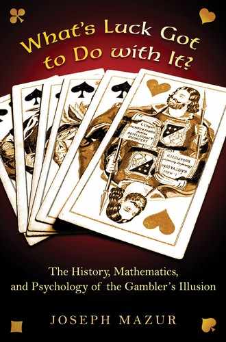
Table 8.1, constructed from knowing the values of p and q for the three different games, shows the probabilities of winning 0, 1, 2, 3, and 4 times in four rounds. In theory, for both roulette and coin flipping, according to table 8.1, a player is most likely to win twice in four rounds. We could construct a table of probabilities for, say, a hundred rounds of roulette and coin flipping, though it would be dauntingly long and impractical. Instead, let me just say that in a hundred rounds of calling heads on the flip of a coin, a player would be most likely to win fifty times, but in a hundred rounds of playing red in roulette he or she would be most likely to win (as we shall see) only forty-seven times. But which forty-seven? Ah, that is the gambler’s Holy Grail. And, as we shall see, it most certainly will not be on the first forty-seven. (It may seem peculiar that in a hundred rounds of playing red in roulette you are only likely to win forty-seven times and not fifty, but that comes from the fact that for roulette p < q and so the peak probability is skewed away from the mean.)
TABLE 8.1
Probabilities of Winning 0, 1, 2, 3, and 4 Times in
Four Rounds of Three Different Games
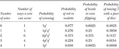
We shall never see that gambler’s Holy Grail. Yet there are things we can know. Amazing things! From table 8.1 we see some symmetry with both roulette and coin flipping, but much less so with dice. If we picture the column for roulette in table 8.1 as a bar graph plotting the number of times red appears versus the probability of getting that number of reds (see figure 8.1), we see a skewed symmetry about the number of wins being 2, while the center of gravity of the graph (the geometric balancing point) seems to be over a number less than 2. When the number of rounds increases to 8 the skew is even more pronounced (see figure 8.2). If we increase the number of roulette rounds to, say, 100, the graph will look smoother. There would then be 101 rectangles, each having a base one unit wide.1
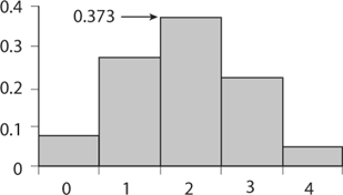
FIGURE 8.1. Probability of winning on red in four rounds of roulette.
FIGURE 8.2. Probability of winning on red in eight rounds of roulette.
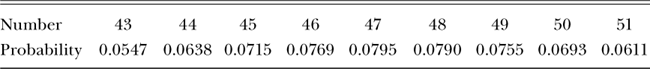
Take a look at figure 8.3. It is what is called a frequency distribution, because the height at each number of successes tells us how frequently those successes are expected to occur. The bars are distributed over the horizontal axis in such a way that the sum of their areas equals 1. A few points to note. Figure 8.3 illustrates the distribution frequency only between the markings 27 and 67. Though the real distribution graph extends from 0 to 100, most of the graph is concentrated between 32 and 62; beyond those marks, the probabilities are spread out so thinly (almost 0) the beginning and end would hardly be seen at a practical scale. (Below 32 and above 62 the probabilities are so small we cannot see them on the graph. For example, P(31) = 0.00034 and P(63) = 0.0006.) It seems a good bet that in 100 rounds of roulette, red will turn up near 47 times (where the highest bar sits). It also tells us that red is much less likely to turn up 20 times or 80 times.
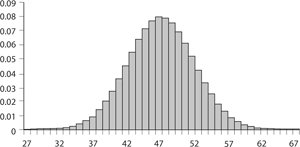
FIGURE 8.3. Probability of winning on red in one hundred rounds of roulette.
One more point. As the number of rounds increases, so does the symmetry. In general, for any games where P(W) is close to P(L), the curve will become more symmetric as the number of rounds increases, but the peak will shift to the left of center if P(W) < P(L); the greater the difference between p and q the bigger the shift. So what could be causing such symmetry and what could be causing the shift? For the answer to the symmetry question, we look at the so-called Pascal triangle (see chapter 2).
In the case of flipping coins, where the probability of heads is also the probability of tails, there is perfect symmetry. In the case of shooting craps there is no symmetry and the probability is largest at zero. This is because the probability of getting 7 is far from the probability of not getting 7.2
The probability that a roulette ball will land on red k times in n rounds is
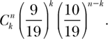
Why? Look at it this way. We first compute the probability that red is hit on every one of the first k spins. Since the probability of hitting red is 9/19, the probability of hitting red k times is (9/19)k. However, we also want exactly k hits in n rounds, so we must also compute the probability of not hitting red on the remaining n – k rounds. Red must happen again and again k times and not happen for n–k times; that is, P(red happening exactly k times in n tries) = P(red)k P(not red)n – k. (Remember that the probability of failure is always 1 minus the probability of success. This is because the success and failure are mutually exclusive and the event must end in either failure or success; i.e., P(Success) + P(failure) = 1.) Hence, the probability of not hitting red on the remaining n – k rounds is (10/19)n – k. Hence the probability of hitting red on every one of the first k rounds is
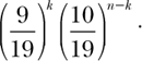
In the end, we don’t really care whether or not red is hit the first k times or the last k times; nor do we care about the order in which red appears in n rounds. So we must multiply 9 19
![]()
by the number of ways k reds can be distributed in n rounds. That number is ![]() . So, the probability of getting exactly k reds in n rounds is
. So, the probability of getting exactly k reds in n rounds is
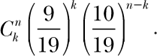
Figure 8.3 displays these n + 1 terms. Note that the height of the middle bar is the probability of getting an even break between red and black, which is computed to be
![]()
Since this number is smaller than the probability of getting 47 reds
![]()
it is more likely that in the course of a hundred trials, the player will not win often enough to get an even break. How clever of the game designers to throw in a green zero and a double zero.
Let us step back to recall what we really wish to measure. Recall that in figure 8.3 the area of the bar (rectangle) above 50 is measuring the probability that the ball will fall into the red pocket 50 times. To find the likelihood of red having an even or better chance, that is, the likelihood that the ball will fall into the red pocket between 50 and 100 times, we simply sum the areas of the rectangles above and between 50 and 100.
Now the bar above 50 represents the probability that in 100 rounds of roulette a player will break even, that is, win as often as lose. Any bar over a number below 50 will give the probability of finishing 100 rounds at a loss—the lower the number, the bigger the loss. We have already calculated that the probability of breaking even is 0.0693. We may calculate the probability of winning k times in 100 rounds by computing
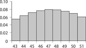
FIGURE 8.4. A modification of figure 8.3.
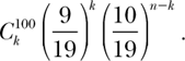
Figure 8.4 is an enlargement of figure 8.3 in the neighborhood of 47. We see that the highest probability on our graph is 0.0795 and that occurs at 47 (see figure 8.4 and table 8.2).
To measure the true probability of ending without a loss, we must sum the areas of all the bars above any number greater than 49, for to do better than break even, we would hope to win any number of times as long as it is a number greater than 50. For that, we must take the sum of all probabilities over 50. Such a calculation would be extremely difficult without the aid of a computer or at least some approximation techniques to simplify the calculations, so you might wonder how probability theorists handled such calculations back in the nineteenth century. A simple computer calculation tells us that the sum of the probabilities from 51 to 100 is
![]()
TABLE 8.2
Probabilities Near the Mean
This is the expectation of doing better than breaking even over the course of 100 rounds. It tells us that at, say, $10 a round and even odds (1 to 1), the average loss over 100 rounds would be $735.
Everything we just said was theory. Until now we have not played real roulette; we have imagined the game played with an ideally spherical ball rolling and bouncing round a flawlessly balanced wheel with precisely spaced pockets in a perfectly steady room in some world we have never seen and that has never existed. That is the theoretical side of what we are about to do. But real wagering takes place in a different world, a physical world where balls and wheels are machined and manufactured to invisibly severe (still imperfect) tolerances by human-made machines built from molecules of atoms with electrons, neutrons, and unnamed subatomic particles. Recall Pearson’s collected observations of 4,274 outcomes of a specific Monte Carlo roulette wheel, where the divergence of theory and practice had odds of a thousand million to one.3 The connection between the ideal and physical is mysterious, and we shall make that connection here.
In the physical world, we could test bona fide roulette wheels for fairness or biases by making a table of observations that could be pictured by a frequency distribution graph. Such a picture may not look anything like the graph of our perfect model, but if the wheel were indeed somewhat fair, and if we were to observe enough rounds, then the graph of observed outcomes would resemble (in shape at least) the graph in figure 8.3. Now, whenever we perform an experiment, we have n outcomes O1, O2, O3 . . . On with respective probabilities p1, p2, p3, . . . pn. This is the observed probability distribution found by knowing the various ways each outcome can occur. Of course, the sum of the n probabilities must be 1, since we would assume that certainty is distributed among all the possible events. To take tossing dice as an example, any one of six faces can be the outcome, each with a probability of 1/6. If the game is fair (i.e., the roulette wheel, die, or coin is unbiased), then the experimental version of the distribution should turn out to resemble the theoretical distribution, though we should expect some discrepancy, as the wheel or die or coin is not a perfect object in a perfect world.
In this context, perfect translates to mathematical. How far from perfect are our observations? That is what we wish to determine, and that shall be done by comparing the data collected by our observations with the data expected in a perfect world. You see, there are gamblers who know that the odds are against them and yet believe that, not infrequently, the physical world wanders from its expectations to favor a random someone; and inevitably, with the powerful thought, someone has to win, those gamblers are willing to risk heavy bets against the mathematical expectations of Fortune.
Let’s hope that the newer wheels of Monte Carlo are fairer than they were at the end of the nineteenth century. After all, Pearson’s observations resembled the expected theory and yet the discrepancy had odds of a thousand million to one! And there is an authentically verified story that sometime in the 1950s a wheel at Monte Carlo came up even twenty-eight times in straight succession. The odds of that happening are close to 268,435,456 to 1. Based on the number of coups per day at Monte Carlo, such an event is likely to happen only once in five hundred years.4
In the first half of the twentieth century (before computers), to make calculations of expectations for a large number of roulette coups, mathematicians would rely on the central limit theorem, which gave an ingenious way to approximate the computation by transforming the distribution bar graph to a smooth graph whose areas to the right of any vertical line were known. Such theoretical approximations are relics of the nineteenth century, when computations of ![]() for k near the range between 30 and 80 would have been quite difficult. We have some notion of this in The Doctrine of Chances, in which the French mathematician Abraham de Moivre tells us that though the solutions to problems of chance often require that some terms of the binomial (a + b)n be added together, very high values of
for k near the range between 30 and 80 would have been quite difficult. We have some notion of this in The Doctrine of Chances, in which the French mathematician Abraham de Moivre tells us that though the solutions to problems of chance often require that some terms of the binomial (a + b)n be added together, very high values of ![]() n tend to present very difficult calculations. The calculations are so difficult, few people have managed them. De Moivre claimed to know of nobody capable of such work besides the two great mathematicians James and Nicolas Bernoulli, who had attempted the problem for high values of n. They did not find the sum exactly, but rather the wide limits within which the sum was contained.5 Today that method is still done as a sentimental habit of the past. There are good reasons for using such methods when dealing with real-life events whose probabilities seem to distribute normally.
n tend to present very difficult calculations. The calculations are so difficult, few people have managed them. De Moivre claimed to know of nobody capable of such work besides the two great mathematicians James and Nicolas Bernoulli, who had attempted the problem for high values of n. They did not find the sum exactly, but rather the wide limits within which the sum was contained.5 Today that method is still done as a sentimental habit of the past. There are good reasons for using such methods when dealing with real-life events whose probabilities seem to distribute normally.
Figure 8.3 contains 101 bars (rectangles). The tops of the bars mark an impression of an almost smooth curve. Such a curve is called a frequency distribution curve because it distributes the frequencies of positive outcomes according to the likelihood p. (The larger the number of bars, the smoother the curve.)
We shall be making a few area-preserving transformations on the curve, and since the areas of the bars represent probabilities, our transformations will continue to preserve probability. Since the base of each bar (rectangle) is one unit in width, the distributions of probabilities are the areas as well as the heights of the rectangles. The transformed graph (figure 8.5) will contain all the information we want to preserve; however, to get a clearer picture of that information we make some simple modifications without altering that information.
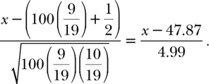
First, we shift the entire graph so that the high point is centered at 0. No information is lost, except that we must interpret the meaning of the new graph. It is now the distribution of probabilities of the incremental increase or decrease of reds over blacks. One further modification: We shrink the curve by a factor of 5 in the vertical direction and magnify it by that same factor in the horizontal direction. (The factor of 5 comes from the computation of ![]() , where N is the number of rounds—in this case 100—p is the probability of getting red, and q is the probability of not getting red. The precise number is 4.99307. It is rounded to 5 for the convenience of instruction.) Of course the vertical axis will no longer represent probability. That job rests with the areas of the rectangles, and those areas have not changed because we magnified the horizontal and contracted the vertical by the same factor.
, where N is the number of rounds—in this case 100—p is the probability of getting red, and q is the probability of not getting red. The precise number is 4.99307. It is rounded to 5 for the convenience of instruction.) Of course the vertical axis will no longer represent probability. That job rests with the areas of the rectangles, and those areas have not changed because we magnified the horizontal and contracted the vertical by the same factor.
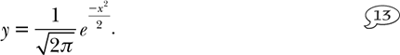
What have we achieved? Here’s the inspired idea. The bar graph that appears in figure 8.3 may be closely approximated by a simple function,
![]()
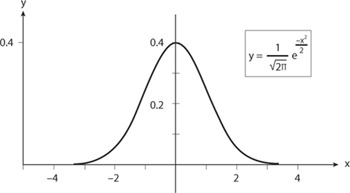
FIGURE 8.5. The graph of ![]() , the standard normal curve.
, the standard normal curve.
where e is the base of the natural logarithm, approximately 2.1718. The graph of that function appears in figure 8.5 and is called the standard normal curve. The important and surprising thing to understand is that this well-studied simple function describes a great many natural phenomena resulting from chance behavior, as long as that function is interpreted correctly.
You may be asking: How can that be? What does this curve—this curve that has no clue that it is modeling events of roulette—have to do with the specific case of balls falling in a red pocket of a roulette wheel? Moreover, you may be amazed to hear that this same curve models coin flipping just as well. The answer is: There is a con, a sleight of hand manipulating the curve that models our particular events by shifting, shrinking, and expanding areas to fit the standard curve, all the while keeping a record of the changes so that no information is lost and that those changes could be translated numerically.
To illustrate the idea, consider the two curves in figures 8.6a and 8.6b. Each has area equal to 1. Each is a transformation of the graph of the function
Just two numbers, the mean μ = 47.9 (where the curve is centered) and the standard deviation σ (the measure of how quickly the curve spreads from the mean), determine the transformation from the curve in figure 8.6a to that in 8.6b. In this case σ = 5.
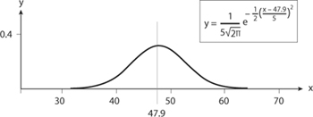
FIGURE 8.6a. Normal curve with μ = 47.9 and σ = 5.
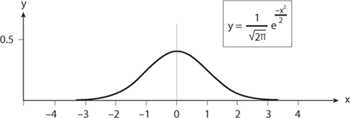
FIGURE 8.6b. Transformation of 8.6a into standard normal curve.
If the graphs look identical, that’s because they are identical. Their difference is in their scales; note the numbers on the axes. However, figure 8.6a came from a specific model of betting red in roulette, whereas figure 8.6b is a general function that seems to have no specific connection to betting red in roulette.
In mathematics as in life, rarely do we get something for free. So, in the end, though things seem so simple, we do have work to do to pay for what we are about to gain. We had to first rigidly shift the graph so its center fell above x = 47.8, the expected number of times a red would turn up in 100 rounds. We had to compute a scalar (a scaling factor) by which to shrink the curve horizontally and magnify it vertically. The computation of both the shift and the scalar involved knowing something about roulette specifically, namely that the probability of success p (the ball falling into a red pocket) is 9/19. Once we had that specific p we were able to compute the scalar as ![]() , where N is the number of rounds, p is the probability of success, and q is the probability of failure (q = 1 – p). In other words, the scalar (the standard deviation) for our particular game of playing red in roulette is
, where N is the number of rounds, p is the probability of success, and q is the probability of failure (q = 1 – p). In other words, the scalar (the standard deviation) for our particular game of playing red in roulette is
![]()
or approximately 5.
Here is how the theory works. Suppose we have a graph of y vs. x. We can make simple transformations of the variables x and y to new variables X and Y;X = x – a, to rigidly slide the original graph a units to the right; X = x/b, to horizontally scale the original graph by a factor of b; and Y = cy, to vertically scale the original graph by a factor of c. Then we have a new graph, Y vs. X. Suppose we have a frequency distribution curve with p relatively close to q. Then we may transform x into X by letting
![]()
and y into Y by letting Y = σy, where μ is the mean and σ is the standard deviation.
By this transformation every binomial frequency curve is transformed (through shifting and scaling) into the standard normal curve
![]()
whose graph appears in figure 8.6b. A magic trick, where this curve comes out of a hat, is something special and powerful. (The discovery of the curve itself goes all the way back to Abraham de Moivre and Pierre-Simon Laplace. It is what you get from the normal distribution
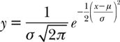
when μ = 0 and σ2 = 1.)
The numbers at the base of the curve in figure 8.6b are counting the numbers of standard deviations from the mean. The horizontal axis is marked in units of standard deviation. Heights on the curve are no longer measures of probability, for they have been scaled, shrunken down to preserve the area under the curve. We get something in return for our work. We know the area over the interval a ≤ X ≤ b is known for any values of a and b. In particular we know that 68 percent of the area lies above the interval –1 ≤ X ≤ 1 and 95 percent of the area lies above –2 ≤ X ≤ 2.
At one standard deviation to the right and left of the curve there are inflection points, where the curve’s S-shape moves along from being concave down to concave up or vice versa. One standard deviation ![]() for a red outcome on a hundred rounds of roulette is not the same as one standard deviation for heads on a hundred rounds of coin flips. So though the curves in each case are similar in form, their interpretations will be different. Nevertheless, the standard normal curve gives us a single model for both roulette and coin flipping. So, though the curve in figure 8.5 may be the same for many different gambling distributions of odds, keep in mind that the markings ±1, ±2, ±3, and the height at the center must be interpreted by specific calculations of the mean and standard deviation, which will depend on the number of rounds, and the likelihood of a positive outcome.
for a red outcome on a hundred rounds of roulette is not the same as one standard deviation for heads on a hundred rounds of coin flips. So though the curves in each case are similar in form, their interpretations will be different. Nevertheless, the standard normal curve gives us a single model for both roulette and coin flipping. So, though the curve in figure 8.5 may be the same for many different gambling distributions of odds, keep in mind that the markings ±1, ±2, ±3, and the height at the center must be interpreted by specific calculations of the mean and standard deviation, which will depend on the number of rounds, and the likelihood of a positive outcome.
As N grows, so does the standard deviation ![]() . However, the standard deviation is measuring how scattered the outcomes are from the mean. Not only is a larger chunk of the horizontal axis grouped under one standard deviation, but also (for a large number of trials) a good deal of the area under the curve will be considered under a single standard deviation from the mean. In the case of our normal standard distribution, 68 percent of the area under the curve is located between one standard deviation to the left of 0 and one standard deviation to the right of 0.
. However, the standard deviation is measuring how scattered the outcomes are from the mean. Not only is a larger chunk of the horizontal axis grouped under one standard deviation, but also (for a large number of trials) a good deal of the area under the curve will be considered under a single standard deviation from the mean. In the case of our normal standard distribution, 68 percent of the area under the curve is located between one standard deviation to the left of 0 and one standard deviation to the right of 0.
What does all this mean? We have translated any deviations from the likelihood of success to the area under one standard curve, a curve we know a great deal about. We know the area below the curve and between the markings. We may now ask how likely certain events are: for example, how likely is it for red to appear between 50 and 70 times in 100 rounds of roulette?
Our simple bell-shaped curve gives us a means of computing the chances of winning at roulette a specified amount over a long string of bets. Sure, the odds are slightly in favor of the casino. And here is where roulette differs from coin flipping. In one round of roulette the expectation of winning is 9/19, the probability of the ball falling into a red pocket. Now 9/19 is deceptively close to 1/2, and many novice gamblers think that with an expected value so close to 1/2, they have close to an even chance of winning. It is true that as the number of rounds increases, the distribution graph more and more resembles the normal distribution curve. But something also happens to offset the expectation. If N is the number of rounds played, the peak of the distribution curve will be (by definition of expected number) above the expected number of wins along the horizontal axis. As N grows that expected number will move further and further toward lower values.
Playing a single round does give almost 1-to-1 odds, but that almost, that slight asymmetry between red and black caused by those two nasty pockets 0 and 00, are keys to casino profits. What happens on the next round and the round after that, or on the fiftieth round? First, we compute the horizontal scaling factor that gets us from our original distribution that was in terms of numbers of rounds to our standard normal distribution that is in terms of standard distributions. That factor is
So x = 50 on our distribution curve corresponds to X = 0.427 on the standard normal curve. We are interested in the area under the standard normal curve to the right of the vertical line through X = 0.427. That area turns out to be 0.3336. Table 8.3 shows the expectations of doing better than breaking even after playing N rounds, assuming each round costs $10. The amounts shown in table 8.3 may not be impressive to someone who may wish to gamble for amusement. However, that gambler should keep in mind that these expectations are all below an even break of 0.5. In other words, luck—if he or she has any—would surely have to work feverishly hard against all the stochastic forces of the casino—not to mention those of the universe—to walk away with any real profit in the long run. And what do I mean by long run? You might say, I don’t stay at the tables long enough to gamble one thousand times. Ah, but remember that that roulette ball doesn’t keep a history of past rolls. If you gamble regularly, one thousand rounds happens before you know it, and it doesn’t matter whether or not you took a break from gambling for a month or a year. Your personal history accounts for the accumulation of your personal gains and losses—it’s always your money added to, or deducted from, net worth.
TABLE 8.3
Expectations of Doing Better Than Breaking after Playing
N Rounds (assuming each round costs $10)
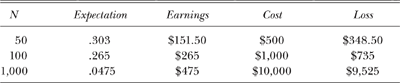
And here’s another thing to keep in mind. Table 8.3 assumes that your bets are fixed at $10 each round. Ha! That’s conservative betting. When you have a gain—and remember that gains are already tabulated in the table—the psyche takes over with great force to compel those chips to compound into the next stake. We shall find out how great that force might be in part 3 of this book. If you win $20, you might be tempted to bet the whole $20 in the next round. This complicates the expected earnings. Gamblers who come with a system, such as the Martingale system of doubling bets on every loss, had better have a large pile of cash ready to lose. Imagine starting with a $10 bet and losing ten times—not likely, but possible. Using this system, that would mean a loss of $10,230. You should be ready to shell out another $10,240 on top of having lost your $5,120. If you happen to win on that eleventh round, your total winnings would be $10.
Okay, so now you argue that expectations are averages, and that some gamblers will win big while others lose big, and that the universe of gamblers together have a negative expectation. Others will look at table 8.1 and declare that it is just as likely that heads stay in the lead for a long run of coin flips; after all, the Dow Jones average does eventually go up. Both points are valid; there are winners. If nobody ever won at roulette, no one would be foolish enough to gamble at roulette and the casinos would close. So occasionally someone wins and, less occasionally, someone wins big time. If not, there is always the image of James Bond to keep believers betting against the odds. He looks so calculating, so dashing and effortless in his tuxedo, holding a dry martini, coolly sliding chip piles to his side. There is something about those luxury casinos, like the one in Monte Carlo, that make us all imagine ourselves as 007.
The man on the street has an impression that the house has a large advantage over players. That may be true for some games, such as slots; however, in general the house advantage is, indeed, as we have seen in the case of roulette, slight. That slight positive edge and large bankroll should be enough—for anyone who understands the mechanism of compounding unfavorable odds—to dissuade the amateur gambler from expecting a profit over longtime play. There really is little hope of beating the house in the face of the law of large numbers. Losses from multiple bets against a house with a slight edge can add up fast.