By now, you should have a good understanding of the importance of indexes. It is equally important for the optimizer to have the necessary statistics on the data distribution so that it can choose indexes effectively. In SQL Server, this information is maintained in the form of statistics on the index key.
In this chapter, you'll learn the importance of statistics in query optimization. Specifically, I cover the following topics:
The importance of statistics on columns with indexes
The importance of statistics on nonindexed columns used in join and filter criteria
Analysis of single-column and multicolumn statistics, including the computation of selectivity of a column for indexing
Statistics maintenance
Effective evaluation of statistics used in a query execution
SQL Server's query optimizer is a cost-based optimizer; it decides on the best data access mechanism and join strategy by identifying the selectivity, how unique the data is, and which columns are used in filtering the data (meaning via the WHERE or JOIN clause). Statistics exist with an index, but they also exist on columns without an index that are used as part of a predicate. As you learned in Chapter 4, you should use a nonclustered index to retrieve a small result set, whereas for data in related sets, a clustered index works better. With a large result set, going to the clustered index or table directly is usually more beneficial.
Up-to-date information on data distribution in the columns referenced as predicates helps the optimizer determine the query strategy to use. In SQL Server, this information is maintained in the form of statistics, which are essential for the cost-based optimizer to create an effective query execution plan. Through the statistics, the optimizer can make reasonably accurate estimates about how long it will take to return a result set or an intermediate result set and therefore determine the most effective operations to use. As long as you ensure that the default statistical settings for the database are set, the optimizer will be able to do its best to determine effective processing strategies dynamically. Also, as a safety measure while troubleshooting performance, you should ensure that the automatic statistics maintenance routine is doing its job as desired. Where necessary, you may even have to take manual control over the creation and/or maintenance of statistics. (I cover this in the "Manual Maintenance" section, and I cover the precise nature of the functions and shape of statistics in the "Analyzing Statistics" section.) In the following section, I show you why statistics are important to indexed columns and nonindexed columns functioning as predicates.
The usefulness of an index is fully dependent on the statistics of the indexed columns; without statistics, SQL Server's cost-based query optimizer can't decide upon the most effective way of using an index. To meet this requirement, SQL Server automatically creates the statistics of an index key whenever the index is created. It isn't possible to turn this feature off.
As data changes, the data-retrieval mechanism required to keep the cost of a query low may also change. For example, if a table has only one matching row for a certain column value, then it makes sense to retrieve the matching rows from the table by going through the nonclustered index on the column. But if the data in the table changes so that a large number of rows are added with the same column value, then using the nonclustered index no longer makes sense. To be able to have SQL Server decide this change in processing strategy as the data changes over time, it is vital to have up-to-date statistics.
SQL Server can keep the statistics on an index updated as the contents of the indexed column are modified. By default, this feature is turned on and is configurable through the Properties
When a table with no rows gets a row
When a table has fewer than 500 rows and is increased by 500 or more rows
When a table has more than 500 rows and is increased by 500 rows + 20 percent of the number of rows
This built-in intelligence keeps the CPU utilization by each process very low. It's also possible to update the statistics asynchronously. This means when a query would normally cause statistics to be updated, instead that query proceeds with the old statistics, and the statistics are updated offline. This can speed up the response time of some queries, such as when the database is large or when you have a short timeout period.
You can manually disable (or enable) the auto update statistics and the auto update statistics asynchronously features by using the ALTER DATABASE command. By default, the auto update statistics feature is enabled, and it is strongly recommended that you keep it enabled. The auto update statistics asynchronously feature is disabled by default. Turn this feature on only if you've determined it will help with timeouts on your database.
Note
I explain ALTER DATABASE later in this chapter in the "Manual Maintenance" section.
The benefits of performing an auto update usually outweigh its cost on the system resources.
To more directly control the behavior of the data, instead of using the tables in AdventureWorks, for this set of examples you will create one manually. Specifically, create a test table (create_t1.sql in the download) with only three rows and a nonclustered index:
IF (SELECT OBJECT_ID('t1')
) IS NOT NULL
DROP TABLE dbo.t1 ;
GO
CREATE TABLE dbo.t1 (c1 INT, c2 INT IDENTITY) ;
SELECT TOP 1500
IDENTITY( INT,1,1 ) AS n
INTO #Nums
FROM Master.dbo.SysColumns sc1
,Master.dbo.SysColumns sc2;
INSERT INTO dbo.t1 (c1)
SELECT n
FROM #Nums
DROP TABLE #Nums
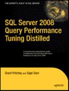
CREATE NONCLUSTERED INDEX i1 ON dbo.t1 (c1) ;If you execute a SELECT statement with a very selective filter criterion on the indexed column to retrieve only one row, as shown in the following line of code, then the optimizer uses a nonclustered index seek, as shown in the execution plan in Figure 7-1:
SELECT * FROM t1 WHERE c1 = 2 --Retrieve 1 row
To understand the effect of small data modifications on a statistics update, create a trace using Profiler. In the trace, add the event Auto Stats, which captures statistics update and create events, and add SQL:BatchCompleted with a filter on the TextData column. The filter should look like Not Like SET% when you are done. Add only one row to the table:
INSERT INTO t1 (c1) VALUES(2)
When you reexecute the preceding SELECT statement, you get the same execution plan as shown in Figure 7-1. Figure 7-2 shows the trace events generated by the query.
The trace output doesn't contain any SQL activity representing a statistics update because the number of changes fell below the threshold where any table that has more than 500 rows must have an increase of 500 rows plus 20 percent of the number of rows.
To understand the effect of large data modification on statistics update, add 1,500 rows to the table (add_rows.sql in the download):
SELECT TOP 1500
        IDENTITY( INT,1,1 ) AS n
INTO    #Nums
FROM    Master.dbo.SysColumns sc1
       ,Master.dbo.SysColumns sc2;
    INSERT INTO dbo.t1 (
        c1
    ) SELECT 2
    FROM #Nums;
DROP TABLE #Nums;
Now, if you reexecute the SELECT statement, like so:
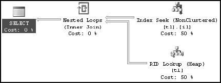
SELECT * FROM dbo.t1 WHERE c1 = 2;
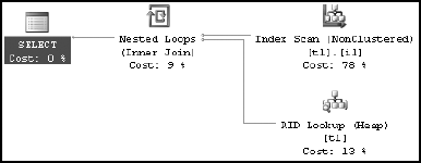
a large result set (1,502 rows out of 3,001 rows) will be retrieved. Since a large result set is requested, scanning the base table directly is preferable to going through the nonclustered index to the base table 1,502 times. Accessing the base table directly will prevent the overhead cost of bookmark lookups associated with the nonclustered index. This is represented in the resultant execution plan (see Figure 7-3).

Figure 7-4 shows the resultant Profiler trace output.
The Profiler trace output includes an Auto Stats event since the threshold was exceeded by the large-scale update this time. These SQL activities consume some extra CPU cycles. However, by doing this, the optimizer determines a better data-processing strategy and keeps the overall cost of the query low.
As explained in the preceding section, the auto update statistics feature allows the optimizer to decide on an efficient processing strategy for a query as the data changes. If the statistics become outdated, however, then the processing strategies decided on by the optimizer may not be applicable for the current data set and thereby will degrade performance.
To understand the detrimental effect of having outdated statistics, follow these steps:
Re-create the preceding test table with 1,500 rows only and the corresponding nonclustered index.
Prevent SQL Server from updating statistics automatically as the data changes. To do so, disable the auto update statistics feature by executing the following SQL statement:
ALTER DATABASE AdventureWorks2008 SET AUTO_UPDATE_STATISTICS OFF
Add 1,500 rows to the table as before.
Now, reexecute the SELECT statement to understand the effect of the outdated statistics on the query optimizer. The query is repeated here for clarity:
SELECT * FROM dbo.t1 WHERE c1 = 2
Figure 7-5 and Figure 7-6 show the resultant execution plan and the Profiler trace output for this query, respectively.
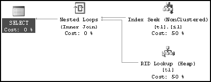
With the auto update statistics feature switched off, the query optimizer has selected a different execution plan from the one it selected with this feature on. Based on the outdated statistics, which have only one row for the filter criterion (c1 = 2), the optimizer decided to use a nonclustered index seek. The optimizer couldn't make its decision based on the current data distribution in the column. For performance reasons, it would have been better to hit the base table directly instead of going through the nonclustered index, since a large result set (1,501 rows out of 3,000 rows) is requested.
You can see that turning off the auto update statistics feature has a negative effect on performance by comparing the cost of this query with and without updated statistics. Table 7-1 shows the difference in the cost of this query.
Table 7.1. Cost of the Query with and Without Updated Statistics
Statistics Update Status | Figure | Cost (SQL:Batch Completed Event) | |
|---|---|---|---|
CPU (ms) | Number of Reads | ||
Updated | 0 | 34 | |
Not updated | 15 | 1509 |
The number of logical reads and the CPU utilization is significantly higher when the statistics are out-of-date even though the data returned is nearly identical and the query was precisely the same. Therefore, it is recommended that you keep the auto update statistics feature on. The benefits of keeping statistics updated outweigh the costs of performing the update. Before you leave this section, turn AUTO_UPDATE_STATISTICS back on (although you can also use sp_autostats):
ALTER DATABASE AdventureWorks2008 SET AUTO_UPDATE_STATISTICS ON
Sometimes you may have columns in join or filter criteria without any index. Even for such nonindexed columns, the query optimizer is more likely to make the best choice if it knows the data distribution (or statistics) of those columns.
In addition to statistics on indexes, SQL Server can build statistics on columns with no indexes. The information on data distribution, or the likelihood of a particular value occurring in a nonindexed column, can help the query optimizer determine an optimal processing strategy. This benefits the query optimizer even if it can't use an index to actually locate the values. SQL Server automatically builds statistics on nonindexed columns if it deems this information valuable in creating a better plan, usually when the columns are used in a predicate. By default, this feature is turned on, and it's configurable through the Properties
In general, you should not disable the automatic creation of statistics on nonindexed columns. One of the scenarios in which you may consider disabling this feature is while executing a series of ad hoc SQL activities that you will not execute again. In such a case, you must decide whether you want to pay the cost of automatic statistics creation to get a better plan in this one case and affect the performance of other SQL Server activities. It is worthwhile noting that SQL Server eventually removes statistics when it realizes that they have not been used for a while. So, in general, you should keep this feature on and not be concerned about it.
To understand the benefit of having statistics on a column with no index, create two test tables with disproportionate data distributions, as shown in the following code (create_t1_t2.sql in the download). Both tables contain 10,001 rows. Table t1 contains only one row for a value of the second column (t1_c2) equal to 1, and the remaining 10,000 rows contain this column value as 2. Table t2 contains exactly the opposite data distribution.
--Create first table with 10001 rows
IF(SELECT OBJECT_ID('dbo.t1')) IS NOT NULL
  DROP TABLE dbo.t1;
GO
CREATE TABLE dbo.t1(t1_c1 INT IDENTITY, t1_c2 INT);
INSERT INTO dbo.t1 (t1_c2) VALUES (1);
SELECT TOP 119026
        IDENTITY( INT,1,1 ) AS n
INTO    #Nums
FROM    Master.dbo.SysColumns sc1
       ,Master.dbo.SysColumns sc2;
    INSERT INTO dbo.t1 (
        t1_c2
    ) SELECT 2
    FROM #Nums
GO
CREATE CLUSTERED INDEX i1 ON dbo.t1(t1_c1)

--Create second table with 10001 rows,
--  but opposite data distribution
IF(SELECT OBJECT_ID('dbo.t2')) IS NOT NULL
  DROP TABLE dbo.t2;
GO
CREATE TABLE dbo.t2(t2_c1 INT IDENTITY, t2_c2 INT);
INSERT INTO dbo.t2(t2_c2) VALUES (2);
    INSERT INTO dbo.t2 (
        t2_c2
    ) SELECT 1
    FROM #Nums;
DROP TABLE #Nums;
GO
CREATE CLUSTERED INDEX i1 ON dbo.t2(t2_c1);
Table 7-2 illustrates how the tables will look.
Table 7.2. Sample Tables
Table t1 | Table t2 | |||
|---|---|---|---|---|
Column | t1_c1 | t1_c2 | t2_c1 | t2_c2 |
| 1 | 1 | 1 | 2 |
| 2 | 2 | 2 | 1 |
| N | 2 | N | 1 |
| 10001 | 2 | 10001 | 1 |
To understand the importance of statistics on a nonindexed column, use the default setting for the auto create statistics feature. By default, this feature is on. You can verify this using the DATABASEPROPERTYEX function (although you can also query the sys.databases view):
SELECT DATABASEPROPERTYEX('AdventureWorks2008', 'IsAutoCreateStatistics')Note
You can find a detailed description of configuring the auto create statistics feature later in this chapter.
Use the following SELECT statement (nonindexed_select.sql in the download) to access a large result set from table t1 and a small result set from table t2. Table t1 has 10,000 rows for the column value of t1_c2 = 2, and table t2 has 1 row for t2_c2 = 2. Note that these columns used in the join and filter criteria have no index on either table.
SELECT  t1.t1_c2
       ,t2.t2_c2
FROM   dbo. t1
        JOIN dbo.t2
        ON t1.t1_c2 = t2.t2_c2
WHERE   t1.t1_c2 = 2;
Figure 7-7 shows the execution plan for this query.
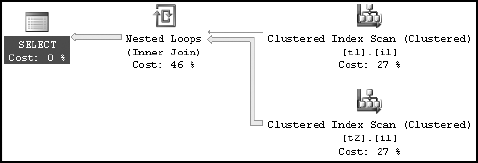
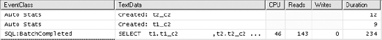
Figure 7-8 shows the Profiler trace output with all completed events and the Auto Stats event for this query. You can use this to evaluate some of the added costs for a given query.
Tip
To keep the Profiler trace output compact, I used a prefilter on TextData Not like SET%. This filters the SET statements used to show the graphical execution plan.
The Profiler trace output shown in Figure 7-8 includes two Auto Stats events creating statistics on the nonindexed columns referred to in the JOIN and WHERE clauses, t2_c2 and t1_c2. This activity consumes a few extra CPU cycles (since none could be detected), but by consuming these extra CPU cycles, the optimizer decides upon a better processing strategy for keeping the overall cost of the query low.
To verify the statistics automatically created by SQL Server on the nonindexed columns of each table, run this SELECT statement against the sys.stats table:
SELECT  *
FROM    sys.stats
WHERE   object_id = OBJECT_ID('t1')
Figure 7-9 shows the automatic statistics created for table t1.
To verify how a different result set size from the two tables influences the decision of the query optimizer, modify the filter criteria of nonindexed_select.sql to access an opposite result set size from the two tables (small from t1 and large from t2). Instead of filtering on t1.t1_c2 = 2, change it to filter on 1:
SELECT  t1.t1_c2
       ,t2.t2_c2
FROM  dbo. t1
        JOIN dbo.t2
        ON t1.t1_c2 = t2.t2_c2
WHERE   t1.t1_c2 = 1
Figure 7-10 shows the resultant execution plan, and Figure 7-11 shows the Profiler trace output of this query.

The resultant Profiler trace output doesn't perform any additional SQL activities to manage statistics. The statistics on the nonindexed columns (t1.t1_c2 and t2.t2_c2) had already been created during the previous execution of the query.
For effective cost optimization, in each case the query optimizer selected different processing strategies, depending upon the statistics on the nonindexed columns (t1.t1_c2 and t2.t2_c2). You can see this from the last two execution plans. In the first, table t1 is the outer table for the nested loop join, whereas in the latest one, table t2 is the outer table. By having statistics on the nonindexed columns (t1.t1_c2 and t2.t2_c2), the query optimizer can create a cost-effective plan suitable for each case.
An even better solution would be to have an index on the column. This would not only create the statistics on the column but also allow fast data retrieval through an Index Seek operation, while retrieving a small result set. However, in the case of a database application with queries referring to nonindexed columns in the WHERE clause, keeping the auto create statistics feature on still allows the optimizer to determine the best processing strategy for the existing data distribution in the column.
If you need to know which column or columns might be covered by a given statistic, you need to look into the sys.stats_columns system table. You can query it in the same way as you did the sys.stats table:
SELECT  *
FROM    sys.stats_columns
WHERE   object_id = OBJECT_ID('t1')
This will show the column or columns being referenced by the automatically created statistics. This will help you if you decide you need to create an index to replace the statistics, because you will need to know which columns to create the statistics on.
To understand the detrimental effect of not having statistics on nonindexed columns, drop the statistics automatically created by SQL Server and prevent SQL Server from automatically creating statistics on columns with no index by following these steps:
Drop the automatic statistics created on column
t1.t1_c2through the Manage Statistics dialog box as shown in the section "Benefits of Statistics on a Nonindexed Column," or use the following SQL command:DROP STATISTICS [t1].StatisticsName
Similarly, drop the corresponding statistics on column
t2.t2_c2.Disable the auto create statistics feature by deselecting the Auto Create Statistics check box for the corresponding database or by executing the following SQL command:
ALTER DATABASE AdventureWorks2008 SET AUTO_CREATE_STATISTICS OFF
Now reexecute the SELECT statement nonindexed_select.sql:
SELECT  t1.t1_c2
       ,t2.t2_c2
FROM   dbo. t1
        JOIN dbo.t2
        ON t1.t1_c2 = t2.t2_c2
WHERE   t1.t1_c2 = 2;
Figure 7-12 and Figure 7-13 show the resultant execution plan and Profiler trace output, respectively.
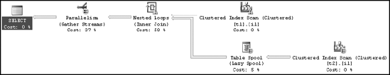
With the auto create statistics feature off, the query optimizer selected a different execution plan compared to the one it selected with the auto create statistics feature on. On not finding statistics on the relevant columns, the optimizer chose the first table (t1) in the FROM clause as the outer table of the nested loop join operation. The optimizer couldn't make its decision based on the actual data distribution in the column. Not only that, but the optimizer and the query engine determined that this query passed the threshold for parallelism, making this a parallel execution (those are the little arrows on the operators, marking them as parallel (more on parallel execution plans in Chapter 9). For example, if you modify the query to reference table t2 as the first table in the FROM clause:
SELECT  t1.t1_c2
       ,t2.t2_c2
FROM   dbo. t2
        JOIN dbo.t1
        ON t1.t1_c2 = t2.t2_c2
WHERE   t1.t1_c2 = 2;
then the optimizer selects table t2 as the outer table of the nested loop join operation. Figure 7-14 shows the execution plan.

You can see that turning off the auto create statistics feature has a negative effect on performance by comparing the cost of this query with and without statistics on a nonindexed column. Table 7-3 shows the difference in the cost of this query.
Table 7.3. Cost Comparison of a Query with and Without Statistics on a Nonindexed Column
Statistics on Nonindexed Column | Figure | Cost (SQL:Batch Completed Event) | |
|---|---|---|---|
Duration (ms) | Number of Reads | ||
With statistics | 159 | 48 | |
Without statistics | 303 | 20,313 |
The number of logical reads and the CPU utilization are very high with no statistics on the nonindexed columns. Without these statistics, the optimizer can't create a cost-effective plan.
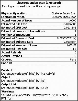
A query execution plan highlights the missing statistics by placing an exclamation point on the operator that would have used the statistics. You can see this in the clustered index scan operators in the previous execution plan (Figure 7-14), as well as in the detailed description in the Warnings section for a node in a graphical execution plan, as shown in Figure 7-15 for table t2.
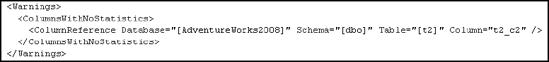
The XML execution plan provides the missing statistics information under the Warnings column, as shown in Figure 7-16. Remember that you can obtain the XML execution plan by right-clicking within the graphical execution plan and selecting Show Execution Plan XML or by using SET STATISTICS XML in the query window.
Note
In a database application, there is always the possibility of queries using columns with no indexes. Therefore, for performance reasons, leaving the auto create statistics feature of SQL Server databases on is recommended.
Statistics are collections of information stored as histograms. A histogram is a statistical construct that shows how often data falls into varying categories. The histogram stored by SQL Server consists of a sampling of data distribution for a column or an index key (or the first column of a multicolumn index key) of up to 200 rows. The information on the range of index key values between two consecutive samples is called a step. These steps consist of varying size intervals between the 200 values stored. A step provides the following information:
The top value of a given step (
RANGE_HI_KEY).The number of rows equal to
RANGE_HI_KEY(EQ_ROWS).The range of rows between the previous top value and the current top value, without counting either of these samples (
RANGE_ROWS).The number of distinct rows in the range (
DISTINCT_RANGE_ROWS). If all values in the range are unique, thenRANGE_ROWSequalsDISTINCT_RANGE_ROWS.The average number of rows equal to a key value within a range (
AVG_RANGE_ROWS).
The value of EQ_ROWS for an index key value (RANGE_HI_KEY) helps the optimizer decide how (and whether) to use the index when the indexed column is referred to in a WHERE clause. Because the optimizer can perform a SEEK or SCAN operation to retrieve rows from a table, the optimizer can decide which operation to perform based on the number of matching rows (EQ_ROWS) for the index key value.
To understand how the optimizer's data-retrieval strategy depends on the number of matching rows, create a test table (create_t3.sql in the download) with different data distributions on an indexed column:
IF (SELECT  OBJECT_ID('dbo.t1')
   ) IS NOT NULL
    DROP TABLE dbo.t1 ;
GO
CREATE TABLE dbo.t1 (c1 INT, c2 INT IDENTITY) ;
INSERT  INTO dbo.t1 (c1)
VALUES  (1) ;
SELECT TOP 119026
        IDENTITY( INT,1,1 ) AS n
INTO    #Nums ;
INSERT  INTO dbo.t1 (c1)
        SELECT  2
        FROM    #Nums ;
CREATE NONCLUSTERED INDEX i1 ON dbo.t1 (c1) ;
When the preceding nonclustered index is created, SQL Server automatically creates statistics on the index key. You can obtain statistics for this nonclustered index key (i1) by executing the DBCC SHOW_STATISTICS command:
DBCC SHOW_STATISTICS(t1, i1)
Figure 7-17 shows the statistics output.
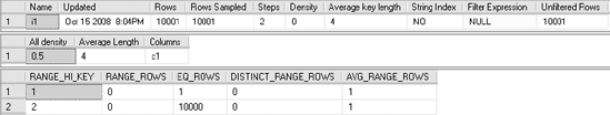
Now, to understand how effectively the optimizer decides upon different data-retrieval strategies based on statistics, execute the following two queries requesting different numbers of rows:
SELECT * FROM dbo.t1 WHERE c1 = 1 --Retrieve 1 row;
SELECT * FROM dbo.t1 WHERE c1 = 2 --Retrieve 10000 rows;
Figure 7-18 shows execution plans of these queries.
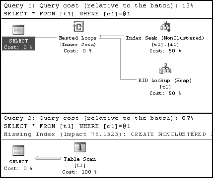
From the statistics, the optimizer can find the number of rows affected by the preceding two queries. Understanding that there is only one row to be retrieved for the first query, the optimizer chose an Index Seek operation, followed by the necessary RID Lookup to retrieve the data not stored with the clustered index. For the second query, the optimizer knows that a large number of rows (10,000 rows) will be affected and therefore avoided the index to attempt to improve performance. (Chapter 4 explains indexing strategies in detail.)
Besides the information on steps, other useful information in the statistics includes the following:
The time statistics were last updated
The number of rows in the table
The average index key length
The number of rows sampled for the histogram
Densities for combinations of columns
Information on the time of the last update can help you decide whether you should manually update the statistics. The average key length represents the average size of the data in the index key column(s). It helps you understand the width of the index key, which is an important measure in determining the effectiveness of the index. As explained in Chapter 4, a wide index is usually costly to maintain and requires more disk space and memory pages.
When creating an execution plan, the query optimizer analyzes the statistics of the columns used in the filter and JOIN clauses. A filter criterion with high selectivity limits the number of rows from a table to a small result set and helps the optimizer keep the query cost low. A column with a unique index will have a very high selectivity, since it can limit the number of matching rows to one.
On the other hand, a filter criterion with low selectivity will return a large result set from the table. A filter criterion with very low selectivity makes a nonclustered index on the column ineffective. Navigating through a nonclustered index to the base table for a large result set is usually costlier than scanning the base table (or clustered index) directly because of the cost overhead of bookmark lookups associated with the nonclustered index. You can observe this behavior in the execution plan in Figure 7-18.
Statistics track the selectivity of a column in the form of a density ratio. A column with high selectivity (or uniqueness) will have low density. A column with low density (that is, high selectivity) is suitable for a nonclustered index, because it helps the optimizer retrieve a small number of rows very fast. This is also the principal on which filtered indexes operate since the filter's goal is to increase the selectivity, or density, of the index.
Density can be expressed as follows:
Density = 1 / Number of distinct values for a column
Density will always come out as a number somewhere between 0 and 1. The lower the column density, the more suitable it is for use in a nonclustered index. You can perform your own calculations to determine the density of columns within your own indexes and statistics. For example, to calculate the density of column c1 from the test table built by create_t3.sql, use the following (results in Figure 7-19):
SELECT 1.0/COUNT(DISTINCT c1) FROM t1
You can see this as actual data in the All density column in the output from DBCC SHOW_STATISTICS. This high-density value for the column makes it a less suitable candidate for an index, even a filtered index. However, the statistics of the index key values maintained in the steps help the query optimizer use the index for the predicate c1 = 1, as shown in the previous execution plan.
In the case of an index with one column, statistics consist of a histogram and a density value for that column. Statistics for a composite index with multiple columns consist of one histogram for the first column only and multiple density values. This is one reason why it's wise to put the more selective column, the one with the lowest density, first when building a compound index or compound statistics. The density values include the density for the first column and for each prefix combination of the index key columns. Multiple density values help the optimizer find the selectivity of the composite index when multiple columns are referred to by predicates in the WHERE and JOIN clauses. Although the first column can help determine the histogram, the final density of the column itself would be the same regardless of column order.
To better understand the density values maintained for a multicolumn index, you can modify the nonclustered index used earlier to include two columns:
CREATE NONCLUSTERED INDEX i1 ON dbo.t1(c1,c2) WITH DROP_EXISTING
Figure 7-20 shows the resultant statistics provided by DBCC SHOW_STATISTICS.
As you can see, there are two density values under the All density column:
The density of the first column
The density of the (first + second) columns
For a multicolumn index with three columns, the statistics for the index would also contain the density value of the (first + second + third) columns. The statistics won't contain a density value for any other combination of columns. Therefore, this index (i1) won't be very useful for filtering rows only on the second column (c2), because the density value of the second column (c2) alone isn't maintained in the statistics.
You can compute the second density value (0.190269999) shown in Figure 7-19 through the following steps. This is the number of distinct values for a column combination of (c1, c2):
SELECT 1.0/COUNT(*)
FROM (SELECT DISTINCT c1, c2 FROM dbo.t1) DistinctRowsThe purpose of a filtered index is to change the data that makes up the index and therefore change the density and histogram to make the index more performant. Instead of a test table, this example will use the AdventureWorks2008 database. Create an index on the Sales. PurchaseOrderHeader table on the PurchaseOrderNumber column:
CREATE INDEX IX_Test ON Sales.SalesOrderHeader (PurchaseOrderNumber)
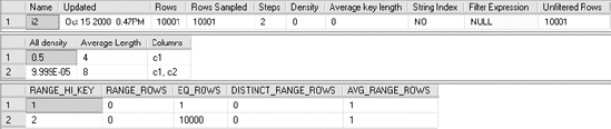
Figure 7-21 shows the header and the density of the output from DBCC SHOW_STATISTICS run against this new index:
DBCC SHOW_STATISTICS('Sales.SalesOrderHeader',IX_Test)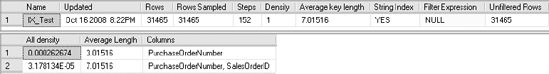
If the same index is re-created to deal with values of the column that are not null, it would look something like this:
CREATE INDEX IX_Test ON Sales.SalesOrderHeader (PurchaseOrderNumber)
WHERE PurchaseOrderNumber IS NOT NULL
WITH DROP_EXISTING
And now, in Figure 7-22, take a look at the statistics information.

First you can see that the number of rows that compose the statistics have radically dropped in the filtered index because there is a filter in place. Notice also that the average key length has increased since you're no longer dealing with zero-length strings. A filter expression has been defined rather than the NULL value visible in Figure 7-21. But the unfiltered rows of both sets of data are the same.
The density measurements are very interesting. Notice that the density is close to the same for both values, but the filtered density is slightly lower, meaning fewer unique values. This is because the filtered data, while marginally less selective, is actually more accurate, eliminating all the empty values that won't contribute to a search. And the density of the second value, which represents the clustered index pointer, is identical with the value of the density of the PurchaseOrderNumber alone because each represents the same amount of unique data. The density of the additional clustered index in the previous column is a much smaller number because of all the unique values of SalesOrderId that are not included in the filtered data because of the elimination of the null values.
One other option open to you is to create filtered statistics. This allows you to create even more fine-tuned histograms on partitioned tables. This is necessary because statistics are not automatically created on partitioned tables and you can't create your own using CREATE STATISTICS. You can create filtered indexes by partition and get statistics or create filtered statistics specifically by partition.
Before going on, clean the indexes created, if any:
DROP INDEX Sales.SalesOrderHeader.IX_Test;
SQL Server allows a user to manually override the maintenance of statistics in an individual database. The four main configurations controlling automatic statistics maintenance behavior of SQL Server are as follows:
New statistics on columns with no index (auto create statistics)
Updating existing statistics (auto update statistics)
The degree of sampling used to collect statistics
Asynchronous updating of existing statistics (auto update statistics async)
You can control the preceding configurations at the levels of a database (all indexes and statistics on all tables) or on a case-by-case basis on individual indexes or statistics. The auto create statistics setting is applicable for nonindexed columns only, because SQL Server always creates statistics for an index key when the index is created. The auto update statistics setting, and the asynchronous version, is applicable for statistics on both indexes and WHERE clause columns with no index.
By default, SQL Server automatically takes care of statistics. Both the auto create statistics and auto update statistics settings are on by default. These two features together are referred to as autostats. As explained previously, it is usually better to keep these settings on. The auto update statistics async setting is off by default.
Auto Create Statistics
The auto create statistics feature automatically creates statistics on nonindexed columns when referred to in the WHERE clause of a query. For example, when this SELECT statement is run against the Sales.SalesOrderHeader table on a column with no index, statistics for the column are created:
SELECT  *
FROM    Sales.SalesOrderHeader AS soh
WHERE   ShipToAddressID = 29692
Then the auto create statistics feature (make sure it is turned back on if you have turned it off) automatically creates statistics on column ShipToAddressID. You can see this in the Profiler trace output in Figure 7-23.
Auto Update Statistics
The auto update statistics feature automatically updates existing statistics on the indexes and columns of a permanent table when the table is referred to in a query, provided the statistics have been marked as out-of-date. The types of changes are action statements, such as INSERT, UPDATE, and DELETE. The threshold for the number of changes depends on the number of rows in the table, as shown in Table 7-4.
Table 7.4. Update Statistics Threshold for Number of Changes
Number of Rows | Threshold for Number of Changes |
|---|---|
0 | > 1 insert |
< 500 | > 500 changes |
> 500 | 500 + 20% of cardinality changes |
In SQL Server, cardinality is counted as the number of rows in the table.
Using an internal threshold reduces the frequency of the automatic update of statistics, and using column changes rather than rows changes further reduces the frequency. For example, consider the following table (create_t4.sql in the download):
IF(SELECT OBJECT_ID('dbo.t1')) IS NOT NULL
    DROP TABLE dbo.t1;
CREATE TABLE dbo.t1(c1 INT);
CREATE INDEX ix1 ON dbo.t1(c1);
INSERT INTO dbo.t1 (
    c1
) VALUES (  0 ) ;
After the nonclustered index is created, a single row is added to the table. This outdates the existing statistics on the nonclustered index. If the following SELECT statement is executed with a reference to the indexed column in the WHERE clause, like so:
SELECT * FROM dbo.t1 WHERE c1 = 0
then the auto update statistics feature automatically updates statistics on the nonclustered index, as shown in the Profiler trace output in Figure 7-24.
Once the statistics are updated, the change-tracking mechanisms for the corresponding tables are set to 0. This way, SQL Server keeps track of the number of changes to the tables and manages the frequency of automatic updates of statistics.
Auto Update Statistics Asynchronously
If auto update statistics asynchronously is set to on, the basic behavior of statistics in SQL Server isn't changed radically. When a set of statistics is marked as out-of-date and a query is then run against those statistics, the statistics update does not interrupt the query, as normally happens. Instead, the query finishes execution using the older set of statistics. Once the query completes, the statistics are updated. The reason this may be attractive is that when statistics are updated, query plans in the procedure cache are removed, and the query being run must be recompiled. So, rather than make a query wait for both the update of the statistics and a recompile of the procedure, the query completes its run. The next time the same query is called, it will have updated statistics waiting for it, and it will have to recompile only.
Although this functionality does make recompiles somewhat faster, it can also cause queries that could benefit from updated statistics and a new execution plan to work with the old execution plan. Careful testing is required before turning this functionality on to ensure it doesn't cause more harm than good.
Note
If you are attempting to update statistics asynchronously, you must also have AUTO_UPDATE_STATISTICS set to ON.
The following are situations in which you need to interfere with the automatic maintenance of statistics:
When experimenting with statistics: Just a friendly suggestion: please spare your production servers from experiments such as the ones you are doing in this book.
After upgrading from a previous version to SQL Server 2008: Since the statistics maintenance of SQL Server 2008 has been upgraded, you should manually update the statistics of the complete database immediately after the upgrade instead of waiting for SQL Server to update it over time with the help of automatic statistics.
While executing a series of ad hoc SQL activities that you won't execute again: In such cases, you must decide whether you want to pay the cost of automatic statistics maintenance to get a better plan in that one case and affect the performance of other SQL Server activities. So, in general, you don't need to be concerned with such one-timers.
When you come upon an issue with the automatic statistics maintenance and the only workaround for the time being is to keep the automatic statistics maintenance feature off: Even in these cases you can turn the feature off for the specific database table that faces the problem instead of disabling it for the complete database.
While analyzing the performance of a query, you realize that the statistics are missing for a few of the database objects referred to by the query: This can be evaluated from the graphical and XML execution plans, as explained earlier in the chapter.
While analyzing the effectiveness of statistics, you realize that they are inaccurate: This can be determined when poor execution plans are being created from what should be good sets of indexes.
SQL Server allows a user to control many of its automatic statistics maintenance features. You can enable (or disable) the automatic statistics creation and update features by using the auto create statistics and auto update statistics settings, respectively, and then you can get your hands dirty.
Manage Statistics Settings
You can control the auto create statistics setting at a database level. To disable this setting, use the ALTER DATABASE command:
ALTER DATABASE AdventureWorks2008 SET AUTO_CREATE_STATISTICS OFF
You can control the auto update statistics setting at different levels of a database, including all indexes and statistics on a table, or at the individual index or statistics level. To disable auto update statistics at the database level, use the ALTER DATABASE command:
ALTER DATABASE AdventureWorks2008 SET AUTO_UPDATE_STATISTICS OFF
Disabling this setting at the database level overrides individual settings at lower levels.
Auto update statistics asynchronously requires that the auto update statistics be on first. Then you can enable the asynchronous update:
ALTER DATABASE AdventureWorks2008 SET AUTO_UPDATE_STATISTICS_ASYNC ON
To configure auto update statistics for all indexes and statistics on a table in the current database, use the sp_autostats system stored procedure:
USE AdventureWorks2008
EXEC sp_autostats 'HumanResources.Department', 'OFF'
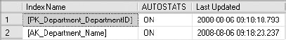
You can also use the same stored procedure to configure this setting for individual indexes or statistics. To disable this setting for the AK_Department_Name index on AdventureWorks2008.HumanResources.Department, execute the following statements:
USE AdventureWorks2008
EXEC sp_autostats 'HumanResources.Department', 'OFF', AK_Department_Name
You can also use the UPDATE STATISTICS command's WITH NORECOMPUTE option to disable this setting for all or individual indexes and statistics on a table in the current database. The sp_createstats stored procedure also has the NORECOMPUTE option. The NORECOMPUTE option will not disable automatic update of statistics directly, but it will prevent them, which is almost the same.
Avoid disabling the automatic statistics features, unless you have confirmed through testing that this brings a performance benefit. If the automatic statistics features are disabled, then you should manually identify and create missing statistics on the columns that are not indexed and then keep the existing statistics up-to-date.
Reset the automatic maintenance of the index so that it is on where it has been turned off:
EXEC sp_autostats 'HumanResources.Department', 'ON'
EXEC sp_autostats 'HumanResources.Department', 'ON', AK_Department_Name
Generate Statistics
To create statistics manually, use one of the following options:
CREATE STATISTICS: You can use this option to create statistics on single or multiple columns of a table or an indexed view. Unlike theCREATE INDEXcommand,CREATE STATISTICSuses sampling by default.sp_createstats: Use this stored procedure to create single-column statistics for all eligible columns for all user tables in the current database. This includes all columns except computed columns; columns with theNTEXT,TEXT,GEOMETRY,GEOGRAPHY, orIMAGEdata type; sparse columns; and columns that already have statistics or are the first column of an index.
Similarly, to update statistics manually, use one of the following options:
You may find that allowing the automatic updating of statistics is not quite adequate for your system. Scheduling UPDATE STATISTICS for the database during off-hours is an acceptable way to deal with this issue. UPDATE STATISTICS is the preferred mechanism because it offers a greater degree of flexibility and control. It's possible, because of the types of data inserted, that the sampling method for gathering the statistics, used because it's faster, may not gather the appropriate data. In these cases, you can force a FULLSCAN so that all the data is used to update the statistics just like what happens when the statistics are initially created. This can be a very costly operation, so it's best to be very selective about which indexes receive this treatment and when it is run.
Note
In general, you should always use the default settings for automatic statistics. Consider modifying these settings only after identifying that the default settings appear to detract from performance.
You can verify the current settings for the autostats feature using the following:
Status of Auto Create Statistics
You can verify the current setting for auto create statistics by running a query against the sys.databases system table:
SELECT is_auto_create_stats_on
FROM sys.databases
WHERE [name] = 'AdventureWorks2008'
A return value of 1 means enabled, and a value of 0 means disabled.
You can also verify the status of this feature using the sp_autostats system stored procedure, as shown in the following code. Supplying any table name to the stored procedure will provide the configuration value of auto create statistics for the current database under the Output section of the global statistics settings:
USE AdventureWorks2008
EXEC sp_autostats 'HumanResources.Department'
Figure 7-25 shows an excerpt of the preceding sp_autostats statement's output.
A return value of ON means enabled, and a value of OFF means disabled.
This stored procedure is more useful when verifying the status of auto update statistics, as explained later in this chapter.
Status of Auto Update Statistics
You can verify the current setting for auto update statistics, and auto update statistics asynchronously, in a similar manner to auto create statistics. Here's how to do it using the function DATABASEPROPERTYEX:
SELECT DATABASEPROPERTYEX('AdventureWorks2008', 'IsAutoUpdateStatistics')Here's how to do it using sp_autostats:
USE AdventureWorks2008
EXEC sp_autostats 'Sales.SalesOrderDetail'
For performance reasons, it is extremely important to maintain proper statistics on your database objects. Issues with statistics are uncommon. However, you still need to keep your eyes open to the possibility of problems with statistics while analyzing the performance of a query. If an issue with statistics does arise, then it can really take you for a ride. In fact, checking that the statistics are up-to-date at the beginning of a query-tuning session eliminates an easily fixed problem. In this section, you'll see what you can do should you find statistics to be missing or out-of-date.
While analyzing an execution plan for a query, look for the following points to ensure a cost-effective processing strategy:
Indexes are available on the columns referred to in the filter and join criteria.
In the case of a missing index, statistics should be available on the columns with no index. It is preferable to have the index itself.
Since outdated statistics are of no use and can even be misleading, it is important that the estimates used by the optimizer from the statistics are up-to-date.
You analyzed the use of a proper index in Chapter 4. In this section, you will analyze the effectiveness of statistics for a query.
To see how to identify and resolve a missing statistics issue, consider the following example. To more directly control the data, I'll use a test table instead of one of the AdventureWorks2008 tables. First, disable both auto create statistics and auto update statistics using the ALTER DATABASE command:
ALTER DATABASE AdventureWorks2008 SET AUTO_CREATE_STATISTICS OFF;
ALTER DATABASE AdventureWorks2008 SET AUTO_UPDATE_STATISTICS OFF;
Create a test table with a large number of rows and a nonclustered index (create_t6.sql in the download):
IF EXISTS ( SELECT  *
            FROM    sys.objects
            WHERE   object_id = OBJECT_ID(N'[dbo].[t1]')
                    AND type IN (N'U') )
    DROP TABLE [dbo].[t1]
GO

CREATE TABLE dbo.t1 (c1 INT, c2 INT, c3 CHAR(50)) ;
INSERT  INTO dbo.t1 (c1, c2, c3)
VALUES  (51, 1, 'c3') ;
INSERT  INTO dbo.t1 (c1, c2, c3)
VALUES  (52, 1, 'c3') ;
CREATE NONCLUSTERED INDEX i1 ON dbo.t1 (c1, c2) ;
SELECT TOP 10000
IDENTITY( INT,1,1 ) AS n
INTO #Nums
FROM Master.dbo.SysColumns sc1
,Master.dbo.SysColumns sc2;
INSERT INTO dbo.t1 (c1, c2, c3)
SELECT n % 50
,n
,'c3'
FROM #Nums;
DROP TABLE #Nums;Since the index is created on (c1, c2), the statistics on the index contain a histogram for the first column, c1, and density values for the prefixed column combinations (c1 and c1 + c2). There are no histograms or density values for column c2.
To understand how to identify missing statistics on a column with no index, execute the following SELECT statement. Since the auto create statistics feature is off, the optimizer won't be able to find the data distribution for the column c2 used in the WHERE clause. You can see this in the execution plan:
SELECT * FROM dbo.t1 WHERE t1.c2 = 1;
If you right-click the execution plan, you can take a look at the XML data behind it. As shown in Figure 7-26, the XML execution plan indicates missing statistics for a particular execution step under its Warnings element. This shows that the statistics on column t1.c2 are missing.
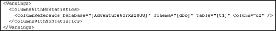
The information on missing statistics is also provided by the graphical execution plan, as shown in Figure 7-27.
The graphical execution plan contains a node with the yellow exclamation point. This indicates some problem with the data-retrieval mechanism (usually missing statistics). You can obtain a detailed description of the error by moving your mouse over the corresponding node of the execution plan to retrieve the tool tip, as shown in Figure 7-28.
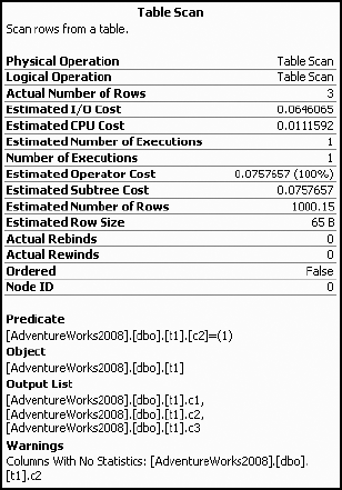
Figure 7-28 shows that the statistics for the column are missing. This may prevent the optimizer from selecting the best processing strategy. The current cost of this query as shown by SET STATISTICS IO and SET STATISTICS TIME is as follows:
Table 't1'. Scan count 1, logical reads 84
SQL Server Execution Times:
   CPU time = 0 ms,  elapsed time = 44 ms.
To resolve this missing statistics issue, you can create the statistics on column t1.c2 by using the CREATE STATISTICS statement:
CREATE STATISTICS s1 ON t1(c2);
Before rerunning the procedure, be sure to clean out the procedure cache because this query will benefit from simple parameterization:
DBCC FREEPROCCACHE();
Figure 7-29 shows the resultant execution plan with statistics created on column c2.
Table 't1'. Scan count 1, logical reads 43
SQL Server Execution Times:
   CPU time = 0 ms,  elapsed time = 15 ms.
The query optimizer uses statistics on a noninitial column in a composite index to determine whether scanning the leaf level of the composite index to obtain the bookmarks will be a more efficient processing strategy than scanning the whole table. In this case, creating statistics on column c2 allows the optimizer to determine that instead of scanning the base table, it will be less costly to scan the composite index on (c1, c2) and bookmark lookup to the base table for the few matching rows. Consequently, the number of logical reads has decreased from 87 to 42, but the elapsed time has decreased only slightly.
Sometimes outdated or incorrect statistics can be more damaging than missing statistics. Based on old statistics or a partial scan of changed data, the optimizer may decide upon a particular indexing strategy, which may be highly inappropriate for the current data distribution. Unfortunately, the execution plans don't show the same glaring warnings for outdated or incorrect statistics as they do for missing statistics.
To identify outdated statistics, you should examine how close the optimizer's estimation of the number of rows affected is to the actual number of rows affected.
The following example shows you how to identify and resolve an outdated statistics issue. Figure 7-30 shows the statistics on the nonclustered index key on column c1 provided by DBCC SHOW_STATISTICS.
DBCC SHOW_STATISTICS(t1, i1);
These results say that the density value for column c1 is 0.5. Now consider the following SELECT statement:
SELECT * FROM dbo.t1 WHERE c1 = 51;
Since the total number of rows in the table is currently 10,002, the number of matching rows for the filter criteria c1 = 51 can be estimated to be 5,001 (= 0.5 × 10,002). This estimated number of rows (5,001) is way off the actual number of matching rows for this column value. The table actually contains only one row for c1 = 51.

You can get the information on both the estimated and actual number of rows from the actual execution plan. An estimated plan refers to and uses the statistics only, not the actual data. This means it can be wildly different from the real data, as you're seeing now. The actual execution plan, on the other hand, has both the estimated and actual number of rows available.
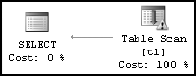
Executing the query results in this execution plan (Figure 7-31) and performance:
Table 't1'. Scan count 1, logical reads 84
SQL Server Execution Times:
   CPU time = 16 ms,  elapsed time = 2 ms.
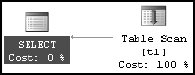
To see the estimated and actual rows, you can view the tool tip by hovering over the Table Scan operator (Figure 7-32).
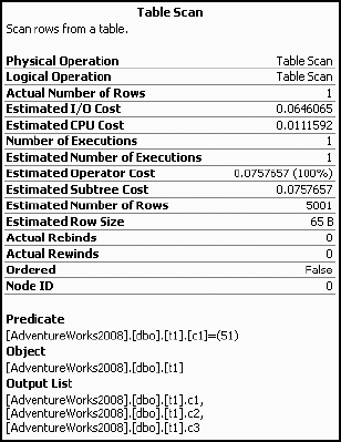
From the estimated rows value vs. the actual rows value, it's clear that the optimizer made an incorrect estimation based on out-of-date statistics. If the difference between the estimated rows and actual rows is more than a factor of 10, then it's quite possible that the processing strategy chosen may not be very cost effective for the current data distribution. An inaccurate estimation may misguide the optimizer in deciding the processing strategy.
To help the optimizer make an accurate estimation, you should update the statistics on the nonclustered index key on column c1 (alternatively, of course, you can just leave the auto update statistics feature on):
UPDATE STATISTICS t1 i1;
If you run the query again, you'll get the following statistics, and the resultant output is as shown in Figure 7-33:
Table 't1'. Scan count 1, logical reads 3
SQL Server Execution Times:
   CPU time = 0 ms,  elapsed time = 0 ms.

The optimizer accurately estimated the number of rows using updated statistics and consequently was able to come up with a plan. Since the estimated number of rows is 1, it makes sense to retrieve the row through the nonclustered index on c1 instead of scanning the base table.
Updated, accurate statistics on the index key column help the optimizer come to a better decision on the processing strategy and thereby reduce the number of logical reads from 84 to 3 and reduce the execution time from 16 ms to ~0 ms (there is a ˜4 ms lag time).
Before continuing, turn the statistics back on for the database:
ALTER DATABASE AdventureWorks2008 SET AUTO_CREATE_STATISTICS ON;
ALTER DATABASE AdventureWorks2008 SET AUTO_UPDATE_STATISTICS ON;
Throughout this chapter, I covered various recommendations for statistics. For easy reference, I've consolidated and expanded upon these recommendations in the sections that follow.
Statistical information in SQL Server 2008 is different from that in previous versions of SQL Server. However, SQL Server 2008 transfers the statistics during upgrade and, by default, automatically updates these statistics over time. For the best performance, however, manually update the statistics immediately after an upgrade.
This feature should usually be left on. With the default setting, during the creation of an execution plan, SQL Server determines whether statistics on a nonindexed column will be useful. If this is deemed beneficial, SQL Server creates statistics on the nonindexed column. However, if you plan to create statistics on nonindexed columns manually, then you have to identify exactly for which nonindexed columns statistics will be beneficial.
This feature should usually be left on, allowing SQL Server to decide on the appropriate execution plan as the data distribution changes over time. Usually the performance benefit provided by this feature outweighs the cost overhead. You will seldom need to interfere with the automatic maintenance of statistics, and such requirements are usually identified while troubleshooting or analyzing performance. To ensure that you aren't facing surprises from the automatic statistics features, it's important to analyze the effectiveness of statistics while diagnosing SQL Server issues.
Unfortunately, if you come across an issue with the auto update statistics feature and have to turn it off, make sure to create a SQL Server job to update the statistics and schedule it to run at regular intervals. For performance reasons, ensure that the SQL job is scheduled to run during off-peak hours.
You can create a SQL Server job to update the statistics from SQL Server Management Studio by following these simple steps:
Select ServerName

On the General page of the New Job dialog box, enter the job name and other details, as shown in Figure 7-34.
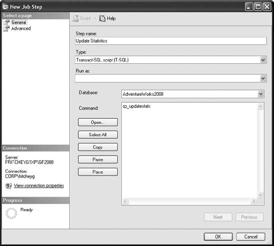
Choose the Steps page, click New, and enter the SQL command for the user database, as shown in Figure 7-35. I used
sp_updatestatshere instead ofUPDATE STATISTICSbecause it's a shortcut. I could have runUPDATE STATISTICSagainst each table in the database a different way, especially if I was interested in taking advantage of all the control offered byUPDATE STATISTICS:EXEC sp_msforeachtable 'UPDATE STATISTICS ? ALL'
Return to the New Job dialog box by clicking the OK button.
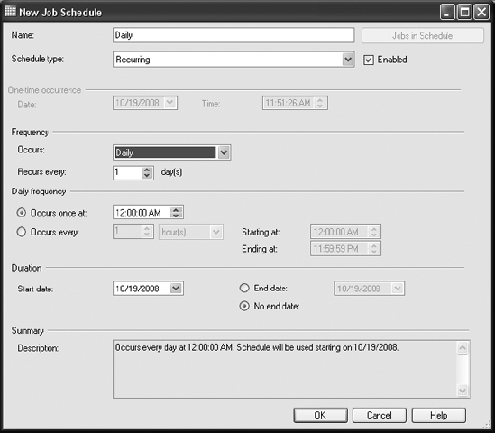
On the Schedules page of the New Job dialog box, click New Schedule, and enter an appropriate schedule to run the SQL Server job, as shown in Figure 7-36.
Return to the New Job dialog box by clicking the OK button.
Once you've entered all the information, click OK in the New Job dialog box to create the SQL Server job.
Ensure that SQL Server Agent is running so that the SQL Server job is run automatically at the set schedule.

Letting statistics update at the beginning of a query, which is the default behavior, will be just fine in most cases. In the very rare circumstances where the statistics update or the execution plan recompiles resulting from that update are very expensive (more expensive than the cost of out-of-date statistics), then you can turn on the asynchronous update of statistics. Just understand that it may mean that procedures that would benefit from more up-to-date statistics will suffer until the next time they are run. Don't forget—you do need automatic update of statistics enabled in order to enable the asynchronous updates.
It is generally recommended that you use the default sampling rate. This rate is decided by an efficient algorithm based on the data size and number of modifications. Although the default sampling rate turns out to be best in most cases, if for a particular query you find that the statistics are not very accurate, then you can manually update them with FULLSCAN.
If this is required repeatedly, then you can add a SQL Server job to take care of it. For performance reasons, ensure that the SQL job is scheduled to run during off-peak hours. To identify cases in which the default sampling rate doesn't turn out to be the best, analyze the statistics effectiveness for costly queries while troubleshooting the database performance. Remember that FULLSCAN is expensive, so you should run it only on those tables or indexes that you've determined will really benefit from it.
As discussed in this chapter, SQL Server's cost-based optimizer requires accurate statistics on columns used in filter and join criteria to determine an efficient processing strategy. Statistics on an index key are always created during the creation of the index, and by default, SQL Server also keeps the statistics on indexed and nonindexed columns updated as the data changes. This enables it to determine the best processing strategies applicable to the current data distribution.
Even though you can disable both the auto create statistics and auto update statistics features, it is recommended that you leave these features on, since their benefit to the optimizer is almost always more than their overhead cost. For a costly query, analyze the statistics to ensure that the automatic statistics maintenance lives up to its promise. The best news is that you can rest easy with a little vigilance, since automatic statistics do their job well most of the time. If manual statistics maintenance procedures are used, then you can use SQL Server jobs to automate these procedures.
Even with proper indexes and statistics in place, a heavily fragmented database will incur an increased data-retrieval cost. In the next chapter, you will see how fragmentation in an index can affect query performance, and you'll learn how to analyze and resolve fragmentation.